5 Hirsch-Fye quantum Monte Carlo method for ... - komet 337

5.20 Nils Blümer
(a) (b)
T
U
X
∆τ=0.25
∆τ=0.15
∆τ=0.10
∆τ=0.00
F [U, T, ∆τ, {G }]
multigrid
HF-QMC
conventional
HF-QMC
{G }
∆τ > 0
∆τ = 0
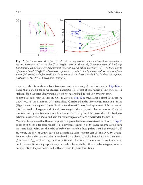
Fig. 12: (a) Scenario for the effect of a∆τ → 0 extrapolation on a metal-insulator coexistence
region, namely a shift to smallerU at roughly constant shape. (b) Schematic view of Ginzburg-
Landau free energy in multidimensional space of hybridization functions{G}. The fixed points
of conventional HF-QMC (diamonds, squares) are adiabatically connected to the exact fixed
point (full circle) only for small ∆τ. In contrast, the multigrid method [45] solves all impurity
problems at the∆τ = 0 fixed point (circles).
may, e.g., shift towards smaller interactions with decreasing ∆τ as illustrated in Fig. 12a, a
phase that is stable for some physical parameter set (cross) at low values of ∆τ may not be
stable at high∆τ (and vice versa), so it cannot be obtained in such ∆τ hysteresis run.
A more abstract view on this problem is given in Fig. 12b: each DMFT fixed point can be
understood as the minimum of a generalized Ginzburg-Landau free energy functional in the
(high-dimensional) space of hybridization functions (full line). In the presence of Trotter errors,
this functional will in general shift and also change its shape, in particular the number of relative
minima. Such phase transition as a function of ∆τ clearly limit the possibilities for hystersis
schemes as discussed above and also for∆τ extrapolation to be discussed in the Sec. 4.
We should also stress that the convergence of a given iteration scheme (such as shown in Fig. 1)
to its fixed point is far from trivial; e.g., a reversed execution of the same scheme would have
the same fixed point, but the roles of stable and unstable fixed points would be reversed.[38]
However, the rate of convergence for a stable iteration scheme can be improved by overrelaxation
where the new solution is replaced by a linear combination with the old solution:
fnew −→ αfnew + (1 − α)fold with α > 0 (while 0 < α < 1 in an underrelaxation scheme
could be used for making a previously unstable scheme stable). While such strategies can save
computer time they are to be used with care close to phase transitions.