5 Hirsch-Fye quantum Monte Carlo method for ... - komet 337

Hirsch-Fye QMC 5.19
Im Σ(i ω n )
0
-0.2
-0.4
-0.6
-0.8
-1
-1.2
-0.9
-1
-1.1
CT-QMC: hybridization
CT-QMC: weak coupling (ω)
HF-QMC: ∆τ=0.4
HF-QMC: ∆τ=0.2
HF-QMC: ∆τ→0
-1.2
0 1 2 3
0 5 10 15 20 25 30 35
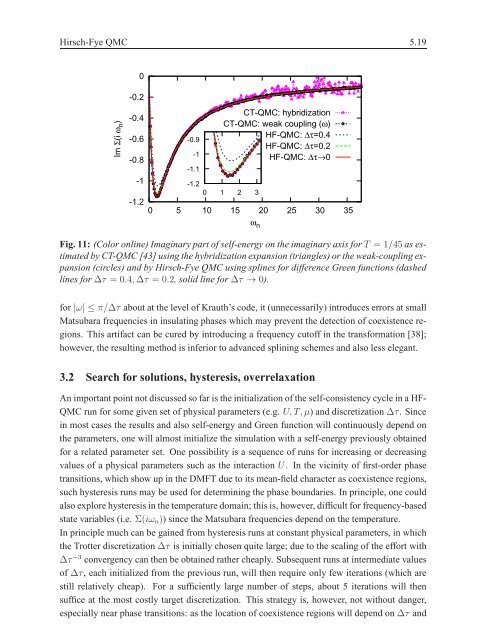
Fig. 11: (Color online) Imaginary part of self-energy on the imaginary axis forT = 1/45 as estimated
by CT-QMC [43] using the hybridization expansion (triangles) or the weak-coupling expansion
(circles) and by Hirsch-Fye QMC using splines for difference Green functions (dashed
lines for∆τ = 0.4,∆τ = 0.2, solid line for∆τ → 0).
for|ω| ≤ π/∆τ about at the level of Krauth’s code, it (unnecessarily) introduces errors at small
Matsubara frequencies in insulating phases which may prevent the detection of coexistence regions.
This artifact can be cured by introducing a frequency cutoff in the transformation [38];
however, the resulting method is inferior to advanced splining schemes and also less elegant.
3.2 Search for solutions, hysteresis, overrelaxation
An important point not discussed so far is the initialization of the self-consistency cycle in a HF-
QMC run for some given set of physical parameters (e.g. U,T,µ) and discretization∆τ. Since
in most cases the results and also self-energy and Green function will continuously depend on
the parameters, one will almost initialize the simulation with a self-energy previously obtained
for a related parameter set. One possibility is a sequence of runs for increasing or decreasing
values of a physical parameters such as the interaction U. In the vicinity of first-order phase
transitions, which show up in the DMFT due to its mean-field character as coexistence regions,
such hysteresis runs may be used for determining the phase boundaries. In principle, one could
also explore hysteresis in the temperature domain; this is, however, difficult for frequency-based
state variables (i.e. Σ(iωn)) since the Matsubara frequencies depend on the temperature.
In principle much can be gained from hysteresis runs at constant physical parameters, in which
the Trotter discretization ∆τ is initially chosen quite large; due to the scaling of the effort with
∆τ −3 convergency can then be obtained rather cheaply. Subsequent runs at intermediate values
of ∆τ, each initialized from the previous run, will then require only few iterations (which are
still relatively cheap). For a sufficiently large number of steps, about 5 iterations will then
suffice at the most costly target discretization. This strategy is, however, not without danger,
especially near phase transitions: as the location of coexistence regions will depend on∆τ and
ω n