5 Hirsch-Fye quantum Monte Carlo method for ... - komet 337

More documents

Recommendations

Info

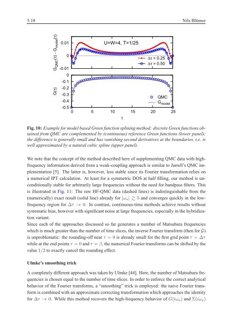
5.18 Nils Blümer G QMC (τ) - G model (τ) G(τ) 0.01 0 -0.01 0 -0.1 -0.2 -0.3 -0.4 -0.5 U=W=4, T=1/25 0 5 10 15 20 25 τ ∆τ = 0.25 ∆τ = 0.50 QMC G model Fig. 10: Example for model based Green function splining method: discrete Green functions obtained from QMC are complemented by (continuous) reference Green functions (lower panel); the difference is generally small and has vanishing second derivatives at the boundaries, i.e. is well approximated by a natural cubic spline (upper panel). We note that the concept of the method described here of supplementing QMC data with highfrequency information derived from a weak-coupling approach is similar to Jarrell’s QMC implementation [5]. The latter is, however, less stable since its Fourier transformation relies on a numerical IPT calculation. At least for a symmetric DOS at half filling, our method is unconditionally stable for arbitrarily large frequencies without the need for bandpass filters. This is illustrated in Fig. 11: The raw HF-QMC data (dashed lines) is indistinguishable from the (numerically) exact result (solid line) already for |ωn| � 5 and converges quickly in the lowfrequency region for ∆τ → 0. In contrast, continuous-time methods achieve results without systematic bias, however with significant noise at large frequencies, especially in the hybridization variant. Since each of the approaches discussed so far generates a number of Matsubara frequencies which is much greater than the number of time slices, the inverse Fourier transform (then forG) is unproblematic: the rounding-off near τ = 0 is already small for the first grid point τ = ∆τ while at the end pointsτ = 0 andτ = β, the numerical Fourier transforms can be shifted by the value1/2 to exactly cancel the rounding effect. Ulmke’s smoothing trick A completely different approach was taken by Ulmke [44]. Here, the number of Matsubara frequencies is chosen equal to the number of time slices. In order to enforce the correct analytical behavior of the Fourier transforms, a “smoothing” trick is employed: the naive Fourier transform is combined with an approximate correcting transformation which approaches the identity for ∆τ → 0. While this method recovers the high-frequency behavior of G(iωn) and Σ(iωn)
Hirsch-Fye QMC 5.19 Im Σ(i ω n ) 0 -0.2 -0.4 -0.6 -0.8 -1 -1.2 -0.9 -1 -1.1 CT-QMC: hybridization CT-QMC: weak coupling (ω) HF-QMC: ∆τ=0.4 HF-QMC: ∆τ=0.2 HF-QMC: ∆τ→0 -1.2 0 1 2 3 0 5 10 15 20 25 30 35 Fig. 11: (Color online) Imaginary part of self-energy on the imaginary axis forT = 1/45 as estimated by CT-QMC [43] using the hybridization expansion (triangles) or the weak-coupling expansion (circles) and by Hirsch-Fye QMC using splines for difference Green functions (dashed lines for∆τ = 0.4,∆τ = 0.2, solid line for∆τ → 0). for|ω| ≤ π/∆τ about at the level of Krauth’s code, it (unnecessarily) introduces errors at small Matsubara frequencies in insulating phases which may prevent the detection of coexistence regions. This artifact can be cured by introducing a frequency cutoff in the transformation [38]; however, the resulting method is inferior to advanced splining schemes and also less elegant. 3.2 Search for solutions, hysteresis, overrelaxation An important point not discussed so far is the initialization of the self-consistency cycle in a HF- QMC run for some given set of physical parameters (e.g. U,T,µ) and discretization∆τ. Since in most cases the results and also self-energy and Green function will continuously depend on the parameters, one will almost initialize the simulation with a self-energy previously obtained for a related parameter set. One possibility is a sequence of runs for increasing or decreasing values of a physical parameters such as the interaction U. In the vicinity of first-order phase transitions, which show up in the DMFT due to its mean-field character as coexistence regions, such hysteresis runs may be used for determining the phase boundaries. In principle, one could also explore hysteresis in the temperature domain; this is, however, difficult for frequency-based state variables (i.e. Σ(iωn)) since the Matsubara frequencies depend on the temperature. In principle much can be gained from hysteresis runs at constant physical parameters, in which the Trotter discretization ∆τ is initially chosen quite large; due to the scaling of the effort with ∆τ −3 convergency can then be obtained rather cheaply. Subsequent runs at intermediate values of ∆τ, each initialized from the previous run, will then require only few iterations (which are still relatively cheap). For a sufficiently large number of steps, about 5 iterations will then suffice at the most costly target discretization. This strategy is, however, not without danger, especially near phase transitions: as the location of coexistence regions will depend on∆τ and ω n
Page 1 and 2: 5 Hirsch-Fye quantum Monte Carlo me
Page 3 and 4: Hirsch-Fye QMC 5.3 notation for the
Page 5 and 6: Hirsch-Fye QMC 5.5 2 Hirsch-Fye QMC
Page 7 and 8: Hirsch-Fye QMC 5.7 withcoshλ = exp
Page 9 and 10: Hirsch-Fye QMC 5.9 (a) (b) 1 0.8 0.
Page 11 and 12: Hirsch-Fye QMC 5.11 the partition f
Page 13 and 14: Hirsch-Fye QMC 5.13 (a) (b) G(τ) 0
Page 15 and 16: Hirsch-Fye QMC 5.15 G(τ) 0 -0.5 0
Page 17: Hirsch-Fye QMC 5.17 be reduced by a
Page 21 and 22: Hirsch-Fye QMC 5.21 4 Computing obs
Page 23 and 24: Hirsch-Fye QMC 5.23 Note the conver
Page 25 and 26: Hirsch-Fye QMC 5.25 (a) 0.0236 (b)
Page 27 and 28: Hirsch-Fye QMC 5.27 1 (a) (b) E (4)
Page 29 and 30: Hirsch-Fye QMC 5.29 A HF-QMC simula
Page 31 and 32: Hirsch-Fye QMC 5.31 The MEM is a ve
Page 33 and 34: Hirsch-Fye QMC 5.33 References [1]
Page 35: Hirsch-Fye QMC 5.35 [43] Emanuel Gu

5 Hirsch-Fye quantum Monte Carlo method for ... - komet 337

Create successful ePaper yourself

Delete template?

Save as template?