5 Hirsch-Fye quantum Monte Carlo method for ... - komet 337

Hirsch-Fye QMC 5.15
G(τ)
0
-0.5
0 1
τ/β
∆τ > 0
∆τ = 0
naive FT
−→
Im G(iω n )
1
0
-1/ω
-1
-3 -2 -1 0
ωn /(π/∆τ)
1 2 3
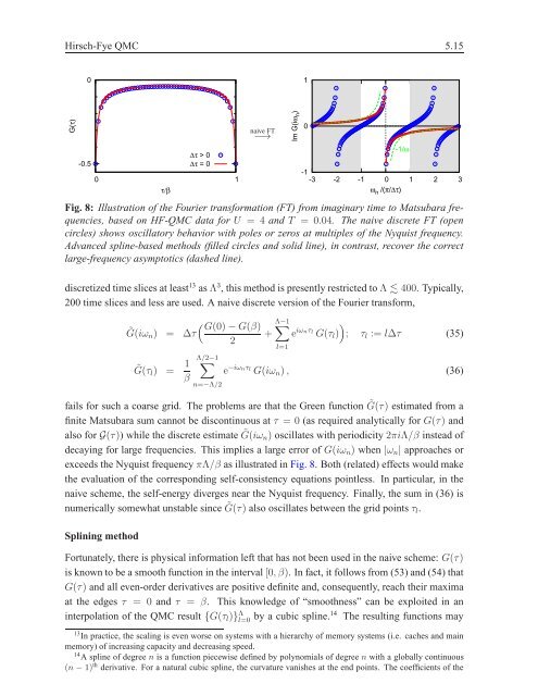
Fig. 8: Illustration of the Fourier transformation (FT) from imaginary time to Matsubara frequencies,
based on HF-QMC data for U = 4 and T = 0.04. The naive discrete FT (open
circles) shows oscillatory behavior with poles or zeros at multiples of the Nyquist frequency.
Advanced spline-based methods (filled circles and solid line), in contrast, recover the correct
large-frequency asymptotics (dashed line).
discretized time slices at least 13 asΛ 3 , this method is presently restricted toΛ � 400. Typically,
200 time slices and less are used. A naive discrete version of the Fourier transform,
�
˜G(iωn)
G(0)−G(β) �Λ−1
= ∆τ + e
2
iωnτl
�
G(τl) ; τl := l∆τ (35)
˜G(τl) = 1
β
Λ/2−1 �
n=−Λ/2
l=1
e −iωnτl G(iωn), (36)
fails for such a coarse grid. The problems are that the Green function ˜ G(τ) estimated from a
finite Matsubara sum cannot be discontinuous at τ = 0 (as required analytically for G(τ) and
also for G(τ)) while the discrete estimate ˜ G(iωn) oscillates with periodicity2πiΛ/β instead of
decaying for large frequencies. This implies a large error of G(iωn) when |ωn| approaches or
exceeds the Nyquist frequencyπΛ/β as illustrated in Fig. 8. Both (related) effects would make
the evaluation of the corresponding self-consistency equations pointless. In particular, in the
naive scheme, the self-energy diverges near the Nyquist frequency. Finally, the sum in (36) is
numerically somewhat unstable since ˜ G(τ) also oscillates between the grid pointsτl.
Splining method
Fortunately, there is physical information left that has not been used in the naive scheme: G(τ)
is known to be a smooth function in the interval[0,β). In fact, it follows from (53) and (54) that
G(τ) and all even-order derivatives are positive definite and, consequently, reach their maxima
at the edges τ = 0 and τ = β. This knowledge of “smoothness” can be exploited in an
interpolation of the QMC result {G(τl)} Λ l=0 by a cubic spline.14 The resulting functions may
13 In practice, the scaling is even worse on systems with a hierarchy of memory systems (i.e. caches and main
memory) of increasing capacity and decreasing speed.
14 A spline of degree n is a function piecewise defined by polynomials of degree n with a globally continuous
(n − 1) th derivative. For a natural cubic spline, the curvature vanishes at the end points. The coefficients of the