A Monte Carlo pencil beam scanning model for proton ... - Creatis

5206 L Grevillot et al
Beam extent σ x (mm)
θ (mrad)
10
5
0
-5
(a)
-10
-150 -100 -50 0 50 100 150
4
2
0
-2
-4
(b)
f(x,y)
-4 -2 0 2 4
x (mm)
1
0.9
0.8
0.7
0.6
0.5
0.4
0.3
0.2
0.1
0
Position along the beam path z (mm)
θ (mrad)
4
2
0
-2
-4
(c)
f(x,y)
-4 -2 0 2 4
x (mm)
1
0.9
0.8
0.7
0.6
0.5
0.4
0.3
0.2
0.1
0
θ (mrad)
4
2
0
-2
-4
(d)
f(x,y)
-4 -2 0 2 4
x (mm)
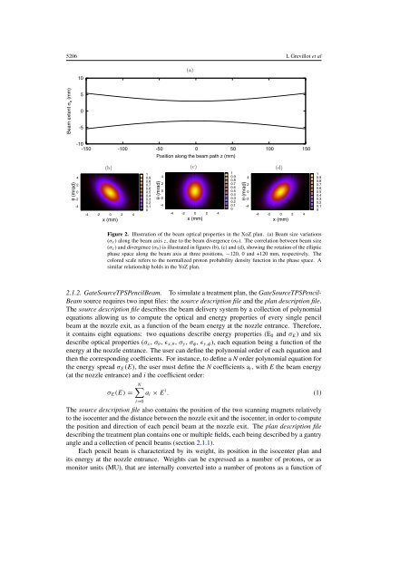
Figure 2. Illustration of the beam optical properties in the XoZ plan. (a) Beam size variations
(σx) along the beam axis z, due to the beam divergence (σθ ). The correlation between beam size
(σx) and divergence (σθ ) is illustrated in figures (b), (c) and (d), showing the rotation of the elliptic
phase space along the beam axis at three positions, −120, 0 and +120 mm, respectively. The
colored scale refers to the normalized proton probability density function in the phase space. A
similar relationship holds in the YoZ plan.
2.1.2. GateSourceTPSPencilBeam. To simulate a treatment plan, the GateSourceTPSPencil-
Beam source requires two input files: the source description file and the plan description file.
The source description file describes the beam delivery system by a collection of polynomial
equations allowing us to compute the optical and energy properties of every single pencil
beam at the nozzle exit, as a function of the beam energy at the nozzle entrance. Therefore,
it contains eight equations: two equations describe energy properties (E0 and σE) and six
describe optical properties (σx, σθ, ɛx,θ, σy, σφ, ɛy,φ), each equation being a function of the
energy at the nozzle entrance. The user can define the polynomial order of each equation and
then the corresponding coefficients. For instance, to define a N order polynomial equation for
the energy spread σE(E), the user must define the N coefficients ai, with E the beam energy
(at the nozzle entrance) and i the coefficient order:
N�
σE(E) = ai × E i . (1)
i=0
The source description file also contains the position of the two scanning magnets relatively
to the isocenter and the distance between the nozzle exit and the isocenter, in order to compute
the position and direction of each pencil beam at the nozzle exit. The plan description file
describing the treatment plan contains one or multiple fields, each being described by a gantry
angle and a collection of pencil beams (section 2.1.1).
Each pencil beam is characterized by its weight, its position in the isocenter plan and
its energy at the nozzle entrance. Weights can be expressed as a number of protons, or as
monitor units (MU), that are internally converted into a number of protons as a function of
1
0.9
0.8
0.7
0.6
0.5
0.4
0.3
0.2
0.1
0