Page Numbering Utility Acrobat4 - Instituto de Informática - UFRGS

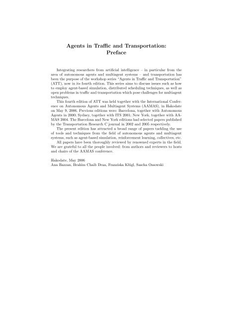
Agents in Traffic and Transportation:
Preface
Integrating researchers from artificial intelligence – in particular from the
area of autonomous agents and multiagent systems – and transportation has
been the purpose of the workshop series “Agents in Traffic and Transportation”
(ATT), now in its fourth edition. This series aims to discuss issues such as how
to employ agent-based simulation, distributed scheduling techniques, as well as
open problems in traffic and transportation which pose challenges for multiagent
techniques.
This fourth edition of ATT was held together with the International Conference
on Autonomous Agents and Multiagent Systems (AAMAS), in Hakodate
on May 9, 2006. Previous editions were: Barcelona, together with Autonomous
Agents in 2000; Sydney, together with ITS 2001; New York, together with AA-
MAS 2004. The Barcelona and New York editions had selected papers published
by the Transportation Research C journal in 2002 and 2005 respectively.
The present edition has attracted a broad range of papers tackling the use
of tools and techniques from the field of autonomous agents and multiagent
systems, such as agent-based simulation, reinforcement learning, collectives, etc.
All papers have been thoroughly reviewed by renowned experts in the field.
We are grateful to all the people involved: from authors and reviewers to hosts
and chairs of the AAMAS conference.
Hakodate, May 2006
Ana Bazzan, Brahim Chaib Draa, Franziska Klügl, Sascha Ossowski

Program Committee
Vicent Botti – UPV (Spain)
Paul Davidsson – BTH (Sweden)
Hussein Dia – University of Queensland (Australia)
Kurt Dresner – University of Texas at Austin (US)
Klaus Fischer – DFKI (Germany)
Josefa Hernandez – Technical Univ. of Madrid (Spain)
Ronghui Liu – University of Leeds (UK)
Kai Nagel – University of Dresden (Germany)
Eugenio de Oliveira – Universidade do Porto (Portugal)
Guido Rindsfüser – Emch&Berger AG Bern (Switzerland)
Rosaldo Rossetti – Universidade Atlantica (Portugal)
Frank Schweitzer – ETH Zuerich (Switzerland)
Joachim Wahle – TraffGo Gmbh (Germany)
Tomohisa Yamashita – National Institute of Advanced Industrial Science and
Technology (AIST), Tokyo, (Japan)
additional reviewer: Minh Nguyen-Duc
Organizing Committee
Ana L. C. Bazzan – UFRGS (Brazil)
Brahim Chaib-draa – Université Laval (Canada)
Franziska Kluegl – Universität Würzburg (Germany)
Sascha Ossowski – Universidad Rey Juan Carlos (Spain)

Contents
Traffic Network Equilibrium using Congestion Tolls: a case study
Bazzan and Junges . . . . . . . . . . . . . . . . . . . . . . . . . . . . . . . . . . . . . . . . . . . . . . . . . . . 1
Agent Architecture for Simulating Pedestrians in the Built Environment
Dijkstra, Jessurun and Vries . . . . . . . . . . . . . . . . . . . . . . . . . . . . . . . . . . . . . . . . . . 8
Human Usable and Emergency Vehicle Aware Control Policies for Autonomous
Intersection Management
Dresner and Stone . . . . . . . . . . . . . . . . . . . . . . . . . . . . . . . . . . . . . . . . . . . . . . . . . . . 17
Cooperative Adaptive Cruise Control: a Reinforcement Learning Approach
Laumonier, Desjardins and Chaib-draa . . . . . . . . . . . . . . . . . . . . . . . . . . . . . . . 26
Multi-Agent Systems as a Platform for VANETs
Manvi, Pitt, Kakkasageri and Rathmell . . . . . . . . . . . . . . . . . . . . . . . . . . . . . . 35
An Agent-Based Simulation Model of Traffic Congestion
McBrenn, Jensen and Marchal . . . . . . . . . . . . . . . . . . . . . . . . . . . . . . . . . . . . . . . 43
MultiAgent Approach for Simulation and Evaluation of Urban Bus Networks
Meignan, Simonin and Koukam . . . . . . . . . . . . . . . . . . . . . . . . . . . . . . . . . . . . . . 50
An Agent Framework for Online Simulation
Miska, Muller and Zuylen . . . . . . . . . . . . . . . . . . . . . . . . . . . . . . . . . . . . . . . . . . . . 57
A Reactive Agent Based Approach to Facility Location: Application to
Transport
Moujahed, Simonin, Koukam and Ghedira . . . . . . . . . . . . . . . . . . . . . . . . . . . . 63
A Fuzzy Neural Approach to Modelling Behavioural Rules in Agent-
Based Route Choice Models
Panwei and Dia . . . . . . . . . . . . . . . . . . . . . . . . . . . . . . . . . . . . . . . . . . . . . . . . . . . . . . 70
Adaptive Traffic Control with Reinforcement Learning
Silva, Oliveira, Bazzan and Basso . . . . . . . . . . . . . . . . . . . . . . . . . . . . . . . . . . . . 80
Invited Paper: Agent Reward Shaping for Alleviating Traffic Congestion
Tumer and Agogino . . . . . . . . . . . . . . . . . . . . . . . . . . . . . . . . . . . . . . . . . . . . . . . . . . 87

Preliminary Program
9:00 – 9:05 Welcome and Short Announcements
9:05 – 10:35 Session I (Autonomous and Cooperative Driving, Reinforcement
Learning)
• 9:05 – 9:35 Human Usable and Emergency Vehicle Aware Control Policies
for Autonomous Intersection Management
• 9:35 – 10:05 Cooperative Adaptive Cruise Control: a Reinforcement Learning
Approach
• 10:05 – 10:35 Adaptive Traffic Control with Reinforcement Learning
10:35 – 11:00 Coffee Break
11:00 – 12:30 Session II (Equilibrium and Collectives)
• 11:00 – 11:40 Invited Talk (K. Tumer)
• 11:40 – 12:00 Traffic Network Equilibrium using Congestion Tolls: a case
study
• 12:00 – 12:30 An Agent-Based Simulation Model of Traffic Congestion
12:30 – 14:00 Lunch Break
14:00 – 15:30: Session III (Information and Agent-based Simulation)
• 14:00 – 14:30 Multi-Agent Systems as a Platform for VANETs
• 14:30 – 15:00 A Fuzzy Neural Approach to Modelling Behavioural Rules in
Agent-Based Route Choice Models
• 15:00 – 15:30 An Agent Framework for Online Simulation
15:30 – 16:00 Coffee Break
16:00 – 17:30 Session IV (Pedestrian and Public Transportation)
• 16:00 – 16:30 Agent Architecture for Simulating Pedestrians in the Built
Environment
• 16:30 – 17:00 MultiAgent Approach for Simulation and Evaluation of Urban
Bus Networks
• 17:00 – 17:30 A Reactive Agent Based Approach to Facility Location: Application
to Transport
17:30 Closing

Traffic Network Equilibrium using Congestion Tolls:
a case study
ABSTRACT
One of the major research directions in multi-agent systems
is learning how to coordinate. When the coordination
emerges out of individual self-interest, there is no guarantee
that the system optimum will be achieved. In fact, in
scenarios where agents do not communicate and only try to
act greedly, the performance of the overall system is compromised.
This is the case of traffic commuting scenarios:
drivers repete their actions day after day trying to adapt to
modifications regarding occupation of the available routes.
In this domain, there has been several works dealing with
how to achieve the traffic network equilibrium. Recently,
the focus has shifted to information provision in several
forms (advanced traveler information systems, route guidance,
etc.) as a way to balance the load. Most of these
works make strong assumptions such as the central controller
(traffic authority) and/or drivers having perfect information.
However, in reality, the information the central
control provides contains estimation errors. The goal of this
paper is to propose a socially efficient load balance by internalizing
social costs caused by agents’ actions. Two issues
are addressed: the model of information provision accounts
for information imperfectness, and the equilibrium which
emerges out of drivers’ route choices is close to the system
optimum due to mechanisms of road pricing. The model can
then be used by traffic authorities to simulate the effects of
information provision and toll charging.
Keywords
User vs. System Optimum, Emergence of Coordination,
Route Choice, Road Pricing for Traffic Management
1. MOTIVATION AND GOALS
In traffic and transportation engineering many control strategies
were developed for different purposes, such as single
intersection control, synchronization of traffic lights in an
arterial, traffic restrictions in roads integrating urban and
freeway traffic, etc. Freeways (highways) were conceived
Ana L. C. Bazzan and Robert Junges
Instituto de Informática, UFRGS
Caixa Postal 15064
91.501-970 Porto Alegre, RS, Brazil
{bazzan,junges}@inf.ufrgs.br
to provide almost unlimited mobility to road users since
freeway traffic has no interruption caused by traffic lights.
However, the increasing demand for mobility in our society
has been causing frequent jams due both to high demand
in peak hours as well as weather conditions and incidents.
As to what regards the former, control measures have been
proposed to better control the utilization of the available
infra-structure [20]: ramp metering (on-ramp traffic lights),
link control (speed limits, lane control, reversable flow, etc.),
and driver information and guidance systems (DIGS).
In this paper we focus on the latter due to the interesting
challenges these systems pose for the area of multiagent systems
in terms of mechanism design, since it involves a very
complex factor: human-made decisions behind the steering
wheel.
Information provision and route guidance strategies may
aim either at achieving the system optimum (minimization
or maximization of some global objective criterion) or the
user optimum. From the point of view of the user, the latter
implies equal costs for all alternative routes connecting two
points in the network. This eventually leads to the system’s
suboptimality. If the focus is on global optimum, then the
route guidance system may eventually recommend a route
which is costlier (for a single user) than it would be the case
if the user optimum were to be recommended. In general,
traffic control authorities are interested in the system optimum,
while the user seeks its own optimum.
One of the challenges of DIGSs and Advanced Travel Information
Systems (ATISs) is to achieve an adequate modeling
and control of traffic flow. This is an issue of ever increasing
importance for dynamic route guidance systems. To be
effective, such systems have to make assumptions about the
travel demand, and hence about travel choices and, especially,
about the behavior of people. It is clear that the
decisions made in reaction to the information an ATIS provides
alter the traffic situation and potentially make the
predictions of the system obsolete.
Although a road user does not reason about social actions
in the narrow sense, traffic systems obviously exhibit social
properties, a kind of N-person coordination game. The interdependence
of actions leads to a high frequency of implicit
coordination decisions. The more reliable the information
that a driver gets about the current and future state of the
traffic network, the more his actions — e.g. his route choice

— depend on what he believes to be the decisions of the
other road users. Especially interesting is the simulation
of learning and self-organized coordination of route choice
which is further detailed in Section 2.1.2.
The aim of the present paper is to investigate the question
of how to include externalities in the utility of drivers in a
commuting scenario. Previous work on this and other issues
related to traffic management and control measures are
briefly presented in the next section. Section 3 introduces
the model based on road pricing as well as discusses the relationship
between the control system and the user/driver.
The mechanism for driver adaptation regarding route choice
is also discussed in this section. Section 4 shows the results
achieved in different scenarios. A conclusion is given in Section
5.
2. RELATED WORK: TRAFFIC AND IN-
FORMATION
2.1 Traffic
In their paper of 1994, Arnott and Small [4] mention the
following figures: about one-third of all vehicular travels
in metropolitan areas of the United States take place under
congested conditions, causing a total delay in trips of
about 6 billion vehicle-hours per year. Despite the fact that
the figures are quite old, the situation has shown no significant
improvement, if any. With costs of extending traffic
networks skyrocketing, policy-makers have to carefully consider
the information provision and behavioral aspects of
the trips, i.e. the drivers behind the steering wheel. Fortunately,
there is also a tendency of reducing that gap: several
researchers are conducting simulations and/or proposing
more realistic models which incorporate information and
behavioral characteristics of the drivers, i.e. how they react
to this information ([3, 8, 9, 18] among others).
There are two main approaches to the simulation of traffic:
macroscopic and microscopic. Both allow for a description of
the traffic elements but the latter considers each road user as
detailed as desired (given computational restrictions), thus
allowing for a model of drivers’ behaviors. Travel and/or
route choices may be considered. This is a key issue in simulating
traffic, since those choices are becoming increasingly
more complex, once more and more information is available.
Multi-agent simulation is a promising technique for both approaches.
Modeling traffic scenarios with multi-agent systems techniques
is not new. However, as to what regards traffic problems
as traffic agents monitoring problem areas (as in [19]),
the focus has been mainly on a coarse-grained level. On the
other hand, our long term work focuses on a fine-grained
level or rather on traffic flow control. Currently, in order to
make traffic simulations at the microscopic level, one may
have to consider travel alternatives (and consequently an extensive
search of information), joint and dynamic decisionmaking,
contingency planning under uncertainty (e.g. due
to congestion), and an increasing frequency of co-ordination
decisions. This has consequences for the behavioral assumptions
on which travel choice models needed to be based. At
this level, there is now an increasing number of research
studies as for example [7, 10, 12, 21, 22, 23].
Therefore, one easily realizes that the multiagent community
is seeking to formalize the necessary combination of methods
and techniques in order to tackle the complexity posed by
simulating and anticipating traffic states. No matter the
motivation behind (training of drivers, forecast, guidance to
drivers, etc.), the approaches seem to converge.
Next, we describe some studies focussing on informed drivers’
decision making. We start with works from the traffic engineering
and traffic economics communities. After, we review
the previous results by one of the authors on iterated route
choice.
2.1.1 Travelers Information System
In Al-Deek and colleagues [1] the goal is to develop a framework
to evaluate the effect of an ATIS. Three types of drivers
are considered: those who are unequipped with electronic
devices of any kind (i.e. they are able to get information
only by observing congestion on site); those who only receive
information via radio; and those equipped only with
an ATIS. The device in the latter case informs drivers about
the shortest travel time route. Some drivers of the first type
are completely unaware of the congestion event. In this case,
they take their usual routes. Average travel time was measured
and it was found that this time improves marginally
with increased market penetration of the ATIS. In general,
the benefits of ATIS are even more marginal when there is
more information available to travelers, especially through
radio, but also through observation. These induce people to
divert earlier to the alternative route.
2.1.2 Iterated Route Choice
A commuting scenario is normally characterized by a driver
facing a repeated situation regarding route selection. Thus,
a scenario of iterated route choice provides a good opportunity
to test learning and emergence of coordination. Of
particular interest is the simulation of learning and selforganized
coordination of route choice. This has been the
focus of the research of one of the authors. The main problem
is to achieve a system’s optimum or at least acceptable
patterns of traffic distribution out of users’ own performance
strategies, i.e. users trying to adapt to the traffic patterns
they experience every day.
There are different means for achieving a certain alignment
of those two objectives (system and user optimum) without
relegating important issues such as traffic information, forecast
and non-commuter users (who possibly do not have any
experience and make random route choices for instance), etc.
A scenario was simulated where N drivers had to select one
of the available routes, in every round. At the end of the
round, every driver gets a reward that is computed based
on the number of drivers who selected the same route, in a
kind of coordination game.
The case of simple user adaptation in a binary route choice
scenario was tackled in [15]. The results achieved were validated
against data from real laboratory experiments (with
subjects playing the role of drivers). To this basic scenario,
traffic forecast was added in [14]. Decisions were made in
two phases: anticipation of route choice based on past experience
(just as above) and actual selection based on a
forecast which was computed by the traffic control system

ased on the previous decision of drivers. In [16] different
forms of traffic information – with different associated costs
– were analyzed. In [5], the role of information sharing was
studied: information was provided by work colleagues, by
acquaintances from other groups (small-world), or by route
guidance systems. Besides, the role of agents lying about
their choices were studied. Finally, information recommendation
and manipulation was tested in [6] with a traffic control
center giving manipulated information for drivers in the
scenario of the Braess Paradox, as a means of trying to divert
drivers to less congested routes. In the Braess Paradox,
the overall travel time can actually increase after the construction
of a new road due to drivers not facing the social
costs of their actions.
The main conclusions of these works were:
• under some circumstances, a route commitment emerges
and the overall system evolves towards equilibrium
while most of the individual drivers learn to select a
given route [15];
• this equilibrium is affected by traffic forecast [14]; however,
forecast implies that the control system must
have at least good estimatives of route choices in order
to compute future traffic state;
• many aspects regarding the type of information as
well as its contents or forms influence the behavior of
drivers; providing different kinds of information may
affect the performances (individual as well as global)
[16];
• it is interesting to have a system giving recommendations
to drivers; however, the performance of the related
people (groups of acquaintances) decreases when
too many drivers deviate from the recommendation;
when there is no social attachment and the behavior
is myopic towards maximization of short time utility,
the performance is worse; information manipulation
may ruin the credibility of the information on the long
run;
• in scenarios such as the Braess Paradox, providing
some kind of route recommendation to drivers can divert
them to a situation in which the effects of the
paradox are reduced [6].
In all these works, different means of utility alignment were
tested. Some were more successful than others as to what
regards performance of the global metrics. However, in the
present paper we want to drop the “perfect information” assumption
(both the traffic control center and all individuals
having knowledge of all alternatives). This assumption is
usually made because there is a gap between the engineering
and behavioral models. Therefore, the traffic models do
not account for the effect of information on the performance
of the system, be it at the global level or the individual one.
Kobayahsi and Do [17] formulate network equilibrium models
with state-dependent congestion tolls in an uncertain environment,
showing that the welfare level of drivers improve.
This is also used in the road pricing scenario as discussed in
the next section.
2.2 Road Pricing
From the perspective of the economics of traffic, Arnott and
Small [4] analyze cases in which the usual measure for alleviating
traffic congestion, i.e. expanding the road system, is
ineffective, as in the case of the Braess Paradox. The resolution
of this and other paradoxes employs the economic
concept of externalities (when a person does not face the
true social cost of an action) to identify and account for the
difference between personal and social costs of using a particular
road. For example, drivers do not pay for the time
loss they impose on others, so they make socially-inefficient
choices. This is a well-studied phenomenon, known more
generally as The Tragedy of the Commons [13]. Besides, it
has been demonstrated that providing information does not
necessarily reduces the level of congestion. One of the reasons
is that naïve information provision can cause the traffic
to be shifted from one route to other alternative(s). This of
course does not improve the global cost balance (system optimum).
Road pricing and specifically congestion tolls are concepts
related to balancing marginal social costs and marginal private
costs (Pigouvian tax). Negative external effects of road
user i over others is in this way accounted for while at the
same time attaining Wardrop’s user equilibrium [24]. It has
been conjectured that road pricing improves the efficiency of
network equilibrium [2]. Besides, congestion tolls convey information
to drivers since they can assess the state of traffic
by means of the amount of toll [11]. In any case, the toll is
calculated by the control center which has the information
about the current traffic situation.
This way, road pricing has been proposed as a way to realize
efficient road utilization i.e. to achieve a distribution of
traffic volume as close as possible to the system optimum.
Congestion toll is one of the road pricing methods: considering
the system optimum, a toll is computed which is the
difference between the marginal social cost and the marginal
private cost. Notice that this difference can be negative,
meaning that drivers actually get a reimbursement. This
mechanism is not to be mistaken with toll charging for the
sake of covering costs of road maintenance or simply for
profit.
Regarding the future traffic situation as well as the effects of
the toll system (and other measures to control the traffic),
most of the work published has assumed that the control
center has perfect information, meaning that it will know
precisely the states of near future traffic conditions. This is
a hard assumption given that acurate weather and accident
forecasts are not possible. Even if they were, other unpredictable
factors alter the state of traffic. Therefore simple
traffic information cannot provide a perfect message to the
driver.
A state-dependent toll pricing system is discussed in [17].
Additionally, they investigate which the impacts of two alternatives
toll schemas are: toll is charged before (ex-ante)
or after (ex-post) drivers select a route. This distinction is
important because congestion tolls, when announced before
drivers make their decisions, carry some meaningful information.
They allow for the calculation of the system optimum
in terms of traffic volume, as well as the drivers expected

welfare (average over all drivers).
In the present paper we compare their results with the distribution
of traffic volume which is achieved when drivers
make their route choices based on the toll they receive, in a
bottom-up, agent-based approach.
3. MODEL
We developed a simple model for the adaptive route choice.
Since an agent has only qualitative information about routes,
and none about other agents, initially, an agent forms an expectation
about the costs he will have if he selects a certain
route. This is achieved by computing the probability with
which a driver selects one route. For instance, if it is 1 for
route r then the driver always takes route r.
With a certain periodicity, driver d updates this heuristics
according to the rewards he has obtained on the routes he
has taken so far. The update of the heuristics is done according
to the following formula:
P
t
heuristics(d,ri) =
utilityri (d, t)
P P
i t utilityr (1)
i (d, t)
The variable utilityr i (d, t) is the reward agent d has accumulated
on route ri up to time t. There is a feedback loop
– the more a driver selects a route, the more information
(in the form of a reward) he gets from this route. Therefore
an important factor is how often the heuristics is updated.
This is particularly relevant since the reward depends on
those of other agents. When the agent is learning, he is also
implicitly adapting himself to the others.
With this model for the driver, we performed experiments by
varying such frequency of heuristics adaptation and focused
on the organization of overall route choice. To prevent that
all agents update their heuristics during the same round,
each agent adapts with a given probability.
In order to model the imperfectness of information, we follow
[3] where traffic conditions are represented as L discrete
states. We also consider K information types. For each
combination of state and information type, there is a cost
function which also depends on the traffic volume. This is
by no means a top-down information. Rather, this is the
signal given to drivers by the environment during the process
of reinforcement learning. Thus, the dynamic selection
of the routes is simulated according to those abstract cost
functions, which nonetheless can reproduce the macroscopic
behavior of the system, given that it includes a stochastic
component regarding the traffic states (ql). This basically
eliminates the need of running actual simulations on a microscopic
simulator in order to account for the actual traffic
flow (as in [16]).
The functions we use were adapted from [17], from which we
also use much of the nomenclature, cost functions, and some
scenarios, althought these were slightly modified to include
the drivers’s adaptation to route choice.
We also assume R alternative routes between two points in
the network. Both have a traffic capacity of M vehicles.
Traffic can be in one of L states (e.g. if L = 2 we can have
congested/non-congested states only). In the model, each
state occurs randomly with probability q l (we use a normal
distribution). The control center predicts traffic based on
imperfect information and provides information to drivers
which is also imperfect. There can be K types of information.
At a given time, one information k is given randomly
with probability p k . There can be any correspondence between
K and L but mostly it is assumed that L ≥ K, K ≥ 2,
and L ≥ 2.
The probability of a state l to occur after information k is
provided is given by π k,l . If π k,l = 1/L, the information
conveys basically no meaning i.e. it is tantamount to no
information. When L = K (i.e. for each k there is an
exclusive l) we can have perfect information provided one
of the π’s is one and the others are zero. For example, if
K = L = 2, when π k,l1 = 1 and π k,l2 = 0 (l1 �= l2), this
is a situation of perfect information provision because it is
known for sure which state is expected to occur after the
information is provided.
3.1 Parameters and Settings
In the examples discussed here, R = K = L = 2, and the
travel cost functions used are linear functions of type c l i =
ζ l i + v l i × x k i , where x is the number of drivers in route i
receiving information k. In particular we use the following
functions [17]:
c 1 1 = 1.0 + 0.6 × 0.001 × x k 1
c 2 1 = 1.5 + 1.6 × 0.001 × x k 2
c 2 1 = 1.0 + 0.4 × 0.001 × x k 1
c 2 2 = 1.5 + 0.1 × 0.001 × x k 1
The meaning of these functions is that the marginal costs
(v l i) of each route ri differ: for state l = 1 this marginal
cost is higher for route 2 than for route 1, whereas for l = 2
the opposite is true. We therefore expect the number of
drivers to be smaller in route 2 when l = 1. In [17] the
system equilibrium (without any toll etc.) is calculated.
When drivers are risk-neutral and the utility is given by
U(y) = −0.1 × y (y being the cost), the system equilibrium
is as shown in Table 1.
k route 1 route 2
1 2391.5 608.5
2 1927.3 1072.7
Table 1: Traffic volumes for system equilibrium
This equilibrium is never achieved when drivers use greedy
strategies such as selection of route based on average of past
travel time, as we show in the next section. However, when
the selection is based on an utility function which includes
the toll paid or the amount reimbursed, then traffic volumes
are close to the system equilibrium.
3.2 Scenarios
To perform the simulations, we use a commuting scenario.
As already mentioned, there are two possible routes, 1 and
2. Depending on the number of drivers that decide to take
route 1, route 2 might be faster. As to what regards drivers
or agents, these go through an adaptation process in which

the probability to select a route is computed based on the
reward they have received given that the specific information
was provided.
In scenario I we are interested in reaching the equilibrium
by only allowing users to apply their probabilities to select
route ri, given the information provision k. In our case this
is done via adaptation of these probabilities (denotated as
ρ d r,k) given the past utilities which are function of the costs
(similarly to what is done with Eq. 1). The basic mechanism
for each driver d is given by:
where U d r,k
ρ d r,k = Ud r,k
RP
U
i=1
d i,k
,1 ≤ i ≤ R (2)
is the average of the past utility for selecting
route ri when the information provided was k.
In scenario II a toll is computed by the traffic control center
and communicated to the driver. This computation is
performed according to information k so that drivers have
to remember their choices made when k was provided. The
toll value for each driver on route ri is calculated as:
where:
τ k r = i xkr − x k∗
r
xk r
x k∗
r i is the number of drivers in the equilibrium situation for
route ri given information k, and x k r i is the expected number
of drivers, estimated by the last time k was provided.
Notice that this value can be positive (driver pays) or negative
(driver gets a reimbursement).
The reasoning of the driver d is:
where:
(3)
• if information k is provided and the last time this happened
I was reimbursed because I chose route ri, then
I had better select ri again with probability ρ d r i,k =
1 − ratecur
• if information k is provided and the last time this has
happened I had to pay, then I select ri with probability
ρ d r i,k = τ d r i,k
• ratecur is the rate of curiosity, i.e. a probability of
d experimenting another route (other than ri) even
though ri was good the last time. In the next section
we show the results for ratecur = 0 and for ratecur =
0.2
• τ d r i,k is the toll paid by driver d when selecting route
ri under information k
2000
1500
1000
500
x=1,k=1
x=2,k=1
x=1,k=2
x=2,k=2
50 100 150 200 250 300
Figure 1: Number of drivers in each route, for each
k; learning happens in every time step
4. RESULTS
In this section we present our simulation results. All quantities
are analyzed as a function of time (1000 simulation steps
which means about 300 trips for each agent on average).
We perform the simulations with M=3000 agents in order to
compare the results to those in [17] since these authors have
calculate the system equilibrium. In the beginning of the
simulation, each agent has equal probabilities of selecting
each one of the routes.
Figure 1 depicts the distribution of drivers between the two
routes, for each information type k. In this case, the adaptation
is made at each time step, i.e. the learning probability
is one for each agent. We have also run simulations with
other learning probabilities without finding significantly different
results, so those graphs are not depicted.
For this scenario, if we let drivers select routes only according
to the utility they perceive (Eq. 1) causing the update of
route choice probability (Eq. 2), then an user’s stable state
is reached. However this is far from the system optimum.
As it is shown in Figure 1, the number of drivers in each
route does not correspond to those in Table 1. For k = 2
the M = 3000 drivers basically select each route with equal
probability, so that nearly 1500 end up on each route at any
given time. This happens because the utility of drivers is
nearly the same when we substitute x k i = 1500 in the cost
functions (cost of each route). For k = 1, the user equilibrium
is two-thirds on route 1 and one-third on route 2. This
equilibrium is never reached: no matter what happens, users
are stuck in a suboptimal stable state. Thus, a mechanism
is needed which internalizes the externalities caused by the
drivers selections.
As already mentioned different mechanisms were applied in
the past with different rates of success. Charging a congestion
toll is a measure that is both a current trend and also
easy to implement since it does not require sophisticated
information provision.
Our scenario II simulates exactly what happens when drivers
update their route choice probabilities according to a utility

2500
2000
1500
1000
500
x=1,k=1
x=2,k=1
x=1,k=2
x=2,k=2
50 100 150 200 250 300
Figure 2: Number of drivers in each route, for each
k; with toll and curiosity rate equal 0
which is based on the past toll (Eq. 3). Figure 2 depicts
the number of drivers in each route, for each k, when a toll
is charged and the curiosity rate is zero. This means that
drivers act only based on the the reward or punishment represented
by the toll the last time information k was provided.
As one can see in that graph, the user equilibrium is now
much closer to the system equilibrium. For k = 1 the distribution
of drivers is around 2300 to 700 (routes 1 and 2
respectively), and for k = 2 this distribution is around 2000
to 1000.
Notice that the deviations are higher here than in scenario
I. This happens because those drivers who got a reimbursement
select one given route with high probability (1−ratecur),
thus causing many people to select the same route. This in
turn increases the toll for it, causing those drivers to divert
to the other route, and so on.
As expected, different rates of curiosity change those previous
figures and how close the system equilibrium is reached.
The higher the rate, the more drivers deviate from the system
equilibrium. For ratecur = 0.2 (20%), the distribution
of drivers is as in Figure 3, meaning that 20% of curious
drivers can cause a high perturbation in the system.
5. CONCLUSION AND OUTLOOK
The main issue tackled in this study is the question of how
to include externalities in the utility of drivers in a commuting
scenario. This is a key issue in traffic control and
management systems as the current infrastructure has to be
used in order to reach optimal utilization. Traffic engineering
normally approaches this problem with top-down solutions,
via calculations of network equilibria etc. However,
when bottom-up approaches such as emergence of behavior
of drivers are considered, other issues such as how these
drivers select a strategy to perform route choice have to be
considered. Normally, drivers tend to use myopic or greedy
strategies which end up causing system suboptimum. This
can be seen in the context of previous works on actual route
choice, as was shown in Section 2.1.2.
The present paper shows that congestion tolls are useful
2000
1500
1000
500
x=1,k=1
x=2,k=1
x=1,k=2
x=2,k=2
50 100 150 200 250 300
Figure 3: Number of drivers in each route, for each
k; with toll and curiosity rate equal 0.2
to internalize the costs drivers impose on others when they
act greedly. It is more efficient than information manipulation
for instance. This method was also simulated by one
of us in a previous paper and despite being effective, it is
sometimes criticized for causing drivers to mistrust the information
system, at least on the long run. Also provision
of traffic forecast was simulated by us with effective results.
However, the forecast depends on the system knowing or estimating
the intentions of drivers regarding the next route
choices.
A congestion toll is a way to somehow punish bad choices
and reward good ones. In commuting scenarios, where drivers
make choices repeatedly, keeping track of the toll paid or received,
given that a certain information was provided, is an
effective way to convey information to drivers. Moreover,
it is the equivalent of the utility alignment proposed in the
COIN framework, but departing from the assumption that
agents are cooperative.
As a final remark, for the context of multiagent systems,
the present work can contribute to the development of a
more general method of mechanism design, specially when
agents are self-interested and the system optimum has to be
reached without imposing explicit central coordination. In
the near future we want to focus on more formal framework
for mechanism design such as auctions protocols in order
to perform comparisons with the present toll mechanism.
However, one concern is that auctions require more communication.
Also, it is not clear whether the decision time is
compatible with real time scenarios.
6. REFERENCES
[1] Al-Deek, H. M., Khattak, A. J., and
Thananjeyan, P. A combined traveler behavior and
system performance model with advanced traveler
information systems. Transportation Research A 32, 7
(September 1998), 479–493.
[2] Arnott, R., de Palma, A., and Lindsey, R.
Departure time and route choice for the morning
commute. Transportation Research B 24 (1990),
209–228.

[3] Arnott, R., de Palma, A., and Lindsey, R. Does
providing information to drivers reduce traffic
congestion? Transportation Research A 25 (1991),
309–318.
[4] Arnott, R., and Small, K. The economics of traffic
congestion. American Scientist 82 (1994), 446–455.
[5] Bazzan, A. L. C., Fehler, M., and Klügl, F.
Learning to coordinate in a network of social drivers:
The role of information. In Proceedings of the
International Workshop on Learning and Adaptation
in MAS (LAMAS) (July 2005), K. Tuyls,
K. Verbeeck, P. J. Hoen, and S. Sen, Eds., pp. 43–57.
[6] Bazzan, A. L. C., and Klügl, F. Case studies on
the Braess paradox: simulating route recommendation
and learning in abstract and microscopic models.
Transportation Research C 13, 4 (August 2005),
299—319.
[7] Bazzan, A. L. C., Wahle, J., and Klügl, F.
Agents in traffic modelling - from reactive to social
behavior. In Advances in Artificial Intelligence
(Berlin/Heidelberg, 1999), no. 1701 in LNAI,
Springer, pp. 303–306. Also appeared as Proc. of the
U.K. Special Interest Group on Multi-Agent Systems
(UKMAS), Bristol, UK.
[8] Ben-Akiva, M., de Palma, A., and Kaysi, I.
Dynamic network models and driver information
systems. Transp. Res. A 25, 5 (1991), 251–266.
[9] Bonsall, P. W., and Parry, T. Using an
interactive route-choice simulator to investigate
driver’s compliance with route guidance advice.
Transportation Research Record 1306 (1991), 59–68.
[10] Dia, H., and Purchase, H. Modelling the impacts of
advanced traveller information systems using
intelligent agents. Road and Transport Research 8
(1999), 68–73.
[11] Do, M., and Kobayashi, K. Route navigation by
state-contigent road pricing. KSCE Journal of Civil
Engineering 4, 3 (2000), 119–128.
[12] Elhadouaj, S., Drogoul, A., and Espié, S. How
to combine reactivity and anticipation: the case of
conflicts resolution in a simulated road traffic. In
Proceedings of the Multiagent Based Simulation
(MABS) (2000), Springer-Verlag New York, pp. 82 –
96.
[13] Hardin, G. The tragedy of the commons. Science 162
(1968), 1243–1248.
[14] Klügl, F., and Bazzan, A. L. C. Route decision
behaviour in a commuting scenario. Journal of
Artificial Societies and Social Simulation 7, 1 (2004).
[15] Klügl, F., and Bazzan, A. L. C. Simulated route
decision behaviour: Simple heuristics and adaptation.
In Human Behaviour and Traffic Networks, R. Selten
and M. Schreckenberg, Eds. Springer, 2004,
pp. 285–304.
[16] Klügl, F., Bazzan, A. L. C., and Wahle, J.
Selection of information types based on personal
utility - a testbed for traffic information markets. In
Proceedings of the Second International Joint
Conference on Autonomous Agents and Multi-Agent
Systems (AAMAS) (Melbourne, Australia, July 2003),
ACM Press, pp. 377–384.
[17] Kobayashi, K., and Do, M. The informational
impacts of congestion tolls upon route traffic
demands. Transportation Research A 39, 7–9
(August-November 2005), 651–670.
[18] Mahmassani, H. S., and Chen, P. S. Comparative
assessment of origin-based and en route real-time
information under alternative user behavior rules.
Transportation Research Record 1306 (1991), 69–81.
[19] Ossowski, S. Co-ordination in artifical agent
societies, social structures and its implications for
autonomous problem-solving agents. No. 1535 in
Lecture Notes in Artificial Intelligence. Springer,
Berlin Heidelberg New York, 1999.
[20] Papageorgiou, M., Diakaki, C., Dinopoulou, V.,
Kotsialos, A., and Wang, Y. Review of road traffic
control strategies. Proceedings of the IEEE 91, 12
(December 2003), 2043–2067.
[21] Paruchuri, P., Pullalarevu, A. R., and
Karlapalem, K. Multi agent simulation of
unorganized traffic. In Proceedings of the First
International Joint Conference on Autonomous Agents
and Multi-Agent Systems (AAMAS) (Bologna, Italy,
2002), vol. 1, ACM Press, pp. 176–183.
[22] Rossetti, R. J. F., Bordini, R. H., Bazzan, A.
L. C., Bampi, S., Liu, R., and Van Vliet, D. Using
BDI agents to improve driver modelling in a
commuter scenario. Transportation Research Part C:
Emerging Technologies 10, 5–6 (2002), 47–72.
[23] Wahle, J., Bazzan, A. L. C., Klügl, F., and
Schreckenberg, M. Decision dynamics in a traffic
scenario. Physica A 287, 3–4 (2000), 669–681.
[24] Wardrop, J. G. Some theoretical aspects of road
traffic research. In Proceedings of the Institute of Civil
Engineers (1952), vol. 2, pp. 325–378.

Agent Architecture for Simulating Pedestrians in the
Built Environment
Jan Dijkstra,Joran Jessurun,Bauke de Vries
Harry Timmermans
Design Systems Group
Urban Planning Group
Eindhoven University of Technology
Eindhoven University of Technology
P.O.Box 513, NL-5600MB Eindhoven
P.O.Box 513, NL-5600MB Eindhoven
+31 40 2472262
+31 40 2472274
{J.Dijkstra,A.J.Jessurun,B.d.Vries}@bwk.tue.nl
H.J.P.Timmermans@bwk.tue.nl
ABSTRACT
The paper discusses an agent architecture for investigating
visualized simulated pedestrian activity and behavior affecting
pedestrian flows within the built environment. The approach will
lead to a system that may serve as a decision support tool in the
design process for predicting the likely impact of design
parameters on pedestrian flows. UML diagrams are used to
communicate about the interpretation of the agent architecture.
1. INTRODUCTION
To date 3D models of the built environment are predominantly
used for presentation of the design to non-professionals and for
design evaluation amongst professionals [35]. Increasingly, such
presentations are done in an interactive and real-time manner,
using VR-based techniques. Although images of humans do occur
in such presentations, these are hardly ever interactive, nor do
they display human behavior. This is all the more striking, as in
architectural and urban design human behavior is the starting
point. Why not test (intermediate) design performances by
simulating human behavior? Therefore, we need virtual persons
that show representative behavior and that allow us to analyze the
performances of the design.
Scientifically, a lot of research is related to the design process by
using virtual humans as substitutes for testing and evaluation
purposes, such as hazard situations, crowding and queuing,
wayfinding, perception, building efficiency, and training.
By allowing virtual humans to populate a design in a specific
situation, behavior of groups as it occurs in 3D space can be
studied in real-time. Such simulation can give valuable feedback
on design performance.
More seriously, we want to take this one step further by
developing a system that relates human behavior to design
parameters. For example, consider the design of a shopping
center. Critical performance indicators related to human behavior
include the distribution of visitors across the center as a function
of layout, and the functional characteristics of the center and its
shops.
The conceptual underpinnings of the system approach are based
on a hybrid approach including cellular automata and agent
technology. The system simulates how agents move around in a
particular 3D environment, in which space is represented as a
lattice of cells with local states, subject to a uniform set of rules,
which drives the behavior of the system. Agents represent
whether virtual humans or more specifically pedestrians with their
own behavior, moving over the network. First, the approach in a
2D environment will be worked out for verifying the
underpinnings.
The paper is organized as follows. First, we will give some
background of the motive of developing a multiagent system for
simulation pedestrian behavior. Next, we discuss some related
research. Than, we will discuss the pedestrian model and agent
structure. Next, we will discuss the simulation of pedestrian
behavior. We will conclude with a brief discussion.
2. BACKGROUND
Since the 1990s, several models of pedestrian movement and
pedestrian traffic flows have been developed. Noticeable is the
success of cellular automata models in various disciplines,
including transportation (e.g. [7,23,29]). Most models are
concerned with pedestrian movement in hazardous situations,
such as evacuation and escape situations (e.g. [19,21,24]). After
the September 11 disaster, great importance has been attached to
these models because the prediction of such behavior is of great
public interest.
In line with this tradition, several years ago we started a research
project that has received the acronym AMANDA, which stands
for A Multi-Agent model for Network Decision Analyses. The
purpose of this research project is to develop a multi-agent system
for network decision analyses [12]. The term network decision
analysis is used to encompass all design and decision problems
that involve predicting how individuals make choices when
moving along a network such as streets and corridors in a
building.
The popularity of cellular automata models is possibly based on
its property that simple principles can be used to successfully
simulate complex traffic flows. A cellular automata model
therefore seemed suitable to simulate other types of movement in
an urban environment. Based on the Nagel-Schreckenberg model
the dynamics of cellular automata models have been investigated
[25,17,5]. The generalization of cellular automata models from
simulated traffic flows to pedestrian movement is considerably
more complicated. While car movements are restricted to lanes,
pedestrian movement is a complex and chaotic process.
Nevertheless, available evidence [6] indicates that cellular
automata models are powerful tools to simulate pedestrian
movement. Road traffic simulation and generation [11,28] as well
as intelligent traveler information systems, traffic management
[20,32,22] and driving agent [16,33,18] systems are subjects in

the context of traffic analysis and finding efficient ways to model
and predict traffic flow.
Previous models of pedestrian behavior have focused primarily on
movement rules, lane forming and crowd dynamics. We want to
extend these models with destination and route choice, and
activity scheduling. To that effect, we started with the basics of
other approaches that have focused on destination and route
choice [8,9]. In these approaches, it was not so much the actual
detailed movement itself, but rather the outcomes of such
movements in terms of destination and route choice that were the
purpose of the modeling process.
We assume that in turn destination and route choice decisions are
influenced by factors such as motivation, activity scheduling,
store awareness, signaling intensity of stores, and store
characteristics.
3. RELATED WORK
Agent-based modeling of pedestrian movement in urban spaces,
especially the implications for the design and modeling of
effective pedestrian environments has been discussed in the
research of Willis et al. [34]. Microscopic movement trajectories
of involved pedestrians were investigated in a video-based
observational study. The results of this study led to a clear insight
into individuals’ movement preferences within uncluttered
environments, desired walking speed, microscopic position
preferences, etc. In other words, insight into movement principles
that are of interest in steering mechanism approach.
Research on multilayered multi-agent situated systems provides a
framework that explicitly defines the spatial structure of the
environment in which a system of situated agents act and interact
[3,4]. With respect to agent behavior, both agent state and
position can be changed by the agent itself according to a
perception-deliberation-action mechanism. In the perception
view, an agent state determines receptiveness and sensitivity.
Receptiveness modulates field intensity and sensitivity filters not
perceivable signals; where field diffusion emits signals that spread
throughout the spatial structure of the environment. At this, we
perceive some correspondence with the AMANDA
environment; signaling intensities of objects can spread
throughout the cellular grid that contains information about agents
and their occupation. Agents can perceive their environment and
sense the information the environment contains.
Nagel [26] pointed out that traffic simulations need to include
other modes of transportation besides car. In a multi-modal
approach a conceptual representation of network layers provisions
for multi-modal trips is explained. Balmer et al. [2] distinguish
two layers of a mobility simulation system: the physical layer and
the mental layer. The physical layer simulates the physical world
where agents move, avoid each other, go around obstacles, etc. In
the mental layer, agents generate strategies, such as routes, mode
choice, daily activity plans, etc. In addition, a feedback is used for
adapting mobility simulation results to the initial mental
condition. Hereby, simulation results are the outcomes of
computing strategies by running the mental module. Starting from
our ideas about activity behavior and movement, we notice some
similarities. An agents’ activity agenda will be updated after an
action selection that influences the movement pattern.
4. PEDESTRIAN MODEL
We want to extend the virtual human behavior approach to a more
generic approach by introducing more behavioral concepts. To
populate an environment with agents representing pedestrians, we
will consider a shopping mall or shopping environment with
shopping pedestrians. Consider a shopping mall or shopping
environment with shopping pedestrians. This environment
consists of streets, which can be represented by a network
consisting of N nodes and L links, and a set of establishments,
consisting of J stores, restaurants, etc. A subset E of these N
nodes represents the entry/departure points of the system. Let us
assume that the pedestrians can be represented by a multiagent
system approach with I agents. Each agent i is supposed to carry
out a set of activities Ai . That is, agents are supposed to purchase
a set of goods, become involved in window-shopping, and
possibly conduct other activities such as having lunch, going to a
movie, etc. We assume that the activity agenda is time-dependent
to allow for changes in the agenda during the trip. The need to
actually realize the various planned activities may differ, partly in
relation to the nature of the trip. If the reason for the trip is
primarily leisure-oriented, the goals and activity agenda may be
relatively fuzzy. In contrast, if the trip is initiated because of some
urgent goal, the need to realize the activity that serves this goal
would be high.
We assume that the completion of an activity is a key decision
point, where agents will adjust, if necessary, their activity agenda
and anticipated time allocation to the activities not yet completed.
Another decision point is every node of the network where agents
may decide to take another route, changing the anticipated
duration of the overall visit in the shopping center.
Agents can perform the activities in a set of J stores or
establishments. Over time, agents form and update beliefs about
these stores. We assume that that these beliefs are a function of
the degree to which the beliefs of the store, driven by their actual
attributes, match the agent's ideals.
In order to implement the activity agenda, the agents need to
successfully visit a set of stores and move over the network. We
assume that the agents' behavior is driven by a series of decision
heuristics. Agents need to decide which stores to choose, in what
order, and which route to take, subject to time and institutional
constraints. We also assume that agents are in different
motivational states. They may at every point during the trip have
general interests in conducting particular activities, without
having decided on the specific store or establishment to visit, but
they may also be in a more goal-directed motivational state in
which case they have already decided which store to visit.
When moving over the network, we assume that agents have
perceptual fields. Perceptual fields may vary according to the
agent's awareness threshold, which in turn may depend on his
motivational state, age, travel party, eye-sight, and the like, and
the signaling intensity of the store, which is assumed a function of
distance, appealing architecture, and whether or not the view is
interrupted by other agents [13].

5. AGENT ARCHITECTURE
5.1 General description
To better communicate our interpretation of agent architecture,
we use UML (Unified Modeling Language) diagrams to guide an
implementation design
Vidal et al. [31] point out that is not trivial to implement common
agent architectures using object-oriented techniques. They make a
UML agent description by figuring out agent features that are
relevant to implementation: unique identity, proactivity,
autonomy, and sociability, inherits its unique identity by being an
object but an agent is more than just a single object. The
mentioned features proactivity, autonomy and sociability have to
do with the common agent notion that an agent perceives its
environment, uses what it perceives to choose an action and then
perform the action.
Agent
-position
-behaviour : BehaviourCollection
-personal characteristics
- . . .
-perceive()
-interpret()
-updEnv()
1
Agenda
*
{ordered}
*
BehaviourCollection
Environment
Activity Establishment
*
0..1
Figure 1. UML diagram of a pedestrian agent
Figure 1 shows the initial concept of a pedestrian agent
description as basis a generic agent structure that can be applied.
By declaring the methods perceive, interpret and updEnv private,
the agent has its own control of the methods. The declaration of
behaviour represents the set of possible attitudes. In this diagram
it is not worked out.
The environment consists of streets, a set of establishments and
pedestrians represented by agents. Streets are presented as a
cellular grid, which is used to simulate agent movement. An agent
moves with his own behavior and personal characteristics. Every
time step, there is an update about agent’s positions. In fact, each
cell in the cellular grid can be considered as an informationcontainer
object. It contains information about the signaling
intensity of an establishment and information about agent’s
positions. We regard a restricted environment E of an agent in the
cellular grid. The cellular grid provides percepts to the agent and
*
the agent performs actions in them. Therefore, we distinguish the
functions perceive and interpret:
Perceive: E � P *
The function perceive represents the perception process of the
agent. It maps the environment E to a set of percepts. The
function interpret represents the decision making process of the
agent and has a more complex form because an agent has an
internal state, which includes the built-in knowledge. The
function interpret is of the following type:
Interpret: P* x I x G � A*
The interpret function maps the perception (P) of the
environment, the current internal sate (I) and the current activity
agenda (G) into a list of one or more actions A, for instance The
interpret function updates the internal state based on its percepts
and the activity agenda; select actions (act) based on the updated
activity agenda and the updated internal state.
UpdStatePandG: P * x I x G � I x G
act: I x G � A *
The function updEnv represents the reaction of the environment
to the agents’ actions.
UpdEnv: E x A * � E
A new state of the environment is realized.
5.2 Basic Agent
Figure 2 represents a UML diagram of the suggested agent
architecture. In particular, the upper part of the diagram provides
the agent description. The Agent class is of the type BasicAgent,
which consists of a Body and a Sensor. This corresponds with
Brooks’ notions about thought and reason [10]. In the discussion
about behavior-based robots, he characterizes among others the
key aspects situatedness and embodiment. In our case, the Body
embodies the object in question in the urban environment, and the
Sensor is needed to observe the visual area. The Body class has
attributes that specify an agent’s position, direction, speed and
other object specific attributes that define its movement in the
regarded environment. The Body class is of the type Vehicle with
basic attributes of its movement through the environment. For its
part, the Vehicle is of the type Movable with a position and
bounding box. In other words, the Body has dimensions and is
movable with a certain speed and direction. The Body implies the
characteristics Situatedness and Embodiment [10]. In our case, the
Body represents a pedestrian, is situated in the world and
experience the world directly.. The suggested description involves
other approaches of body, for instance driver.
Furthermore, the Agent will be driven by the Brain. It reflects the
relationship between the mind and the brain. What is perception
and how is it related to the object perceived. While the mind
remains a mysterious and inaccessible phenomenon, many
components of the mind, such as perception, behavior generation,
knowledge representation, value judgment, reason, intention,
emotion, memory, imagination, recognition, learning, attention,
and intelligence are becoming well defined and amenable to
analysis.[1].

Agent
+enabled : boolean
+hasMobable()
+getMovable()
+step()
+Interpret()
+Perceive()
+SetUpdEnv()
Brai
+addLobe()
+getLobe() : «abstract»
Lobe
+step()
*
«abstract»
«abstract»
Lobe
+getId()
+getLobes(in lobeId) : Lobes
RoutingLobe
-walkleft
-walkright
+generatePath()
MentalMap
1
BasicAgent
+hasVehicle()
+getVehicle()
ActivityPlanningLobe
1
*
Sensor
In this way, the Brain consists of functional elements. On the
one hand, behavior generation such as the planning and control
of action designed to achieve behavioral goals, on the other
hand sensory perception for the transformation of data into
meaningful and useful representations of the world. We assume
the Brain class consists of active and passive lobes that can be
extended with other lobe such as ShoppingLobe that is not
included in the diagram. Active lobes are lobes for which the
step function will be called regularly; they are continuously
active. On the other hand, Passive lobes must be triggered
before its specific functionality getting active. Subtypes of the
ActiveLobe class are among others the SteeringLobe class
which drives steering behavior; which differs from agent to
agent. The SteeringBehaviour class is connected with the
Body
+maxspeed
+fatigue
+maxacceleration
+maxturnspeed
*
«abstract»
ActiveLobe
+priority : int
+active : bool
+step()
SteeringLobe
-steeringBehaviour : SteeringBehaviour
+setPath()
«event» +onNodeArrival()
Path
Figure 2. Agent Diagram
*
Vehicle
+speed
+acceleration
+turnspeed
+velocity
+direction
PathNode
-width: float
SteeringBehaviour
Movable
-position : Vector
-collidable : boolean
-shape
+getBoundingBox()
+getBoundingSphere()
«event» +onMove()
SteeringLobe class (quoted as 1. in figure 2.). Herein, the
SteeringActuator class executes a behavior and let an assigned
vehicle move according to that behavior.
Other subtypes of the ActiveLobe class are the
PlanCheckerLobe, the SensingLobe class, and the
ConductActivityLobe class. PlanCheckerLobe checks if the
activity schedule needs to be updated because the current plan is
not accurate or viable anymore. SensingLobe will be a special
event generation system. ConductActivityLobe simulates doing
an activity. Subtypes of the passive Lobe class are the
RoutingLobe class and the ActivityPlanningLobe class.
RoutingLobe uses visible data from the neighborhood and data
in memory for parts of the environment that are not visible to
1

plan routes. The ActivityPlanningLobe makes up an activity
schedule.
5.3 Steering Behavior
Graphs are used for path finding to a specific location in the
environment; each node of the graph has a corresponding
location in the environment. When using graphs as mental map
of virtual humans, the graph can be part of the virtual
environment and thus identical for all its inhabitants or it can be
constructed by each virtual human individually. In the last case
nodes as possible location to go, must be generated by the
system, for instance as grid points that are flooded over the
environment.
The cellular grid divides the environment in cells. Each cell has
one or more attributes to express physical conditions (e.g. wall)
or a state (e.g. occupied). Steering is implemented by moving
through the grid and meanwhile inspecting the neighborhood
cells. Dependent on the physical condition and the state of cell
the decision is made whether or not moving on in that direction
is possible. Evidently the environment and its occupying objects
must neatly be fitted in the grid, which is not always trivial (e.g.
curved objects).
Figure 3. Steering Diagram
Figure 3 shows the steering behavior diagram; the
SteeringBehaviour class determines the existence of the vehicle
and how behavior is assigned to that vehicle. SteeringActuator
executes a behavior and an assigned vehicle moves according to
that behavior which includes all checks and the movement itself.
The composite design pattern SteeringComposition indicates
how the different SteeringBehaviours are coordinated. The
steering behavior diagram is the base of the steering algorithm
and contains different methods of combining steering behaviors
and is extendable. The steering algorithm will make use of the
properties to determine its behavior but also the composition of
steering behaviors will influence the way the steering will work.
Vehicles use steering behavior including (i) path following to
follow paths generated by path generation algorithms, (ii)
unaligned collision avoidance to avoid collisions with moving
objects or agents, (iii) obstacle avoidance or containment to
avoid bumping into static obstacles and buildings, and (iv) non
penetration constraint to avoid vehicles to overlap with each
other or obstacles. The steering module will complete integrate
with the environment. Figure 4 shows a simplified steering
object diagram.

5.4 Environment model
In the AMANDA model system, we populate an environment
representing pedestrians. Polygons are used to indicate borders
and functional areas like walkways. Discretisation of these
polygons generates a grid of cells, which is called a cellular
grid. Therefore, a cellular grid together with the polygons
represents the environment. Each cell in the cellular grid can be
considered as an information container object. It has information
Figure 4. Steering Object Diagram
Figure 5. Environment Diagram
about which agents and polygons occupy it. Also, it contains
information about other features such as appearance
characteristics or establishments that are observable from that
cell.
Figure 5 shows the environment diagram. The environment class
consists of a cellular grid and a Layer class. Movables can be
positioned in cells of the grid. The environment will use layers
to classify the meaning of the containing polygons.

We suggest a dual definition of the environment. The
environment is defined using polygons with a reference to one
information object for each polygon. Otherwise, the
environment is described as a lattice of cells. Each cell
references to an information object. Often, a lot of cells will
reference to the same information object, simply because for
example a stroe will be made up of multiple cells. Also a cell
could involve information about the attraction of a store, smell,
noise, etc. Cells nearby the store have a more noticeable
perception than cells farther away.
6. PEDESTRIAN SIMULATION
Two aspects are relevant for understanding the simulation of
individual pedestrian behavior: steering including path
determination, and action selection including strategy, goal
formulation and planning.
Action selection � Steering � Movement
6.1 Action selection
We assume that pedestrian movement is embedded in the larger
problem of activity scheduling [30]. It is assumed that
individuals made decisions regarding their activity agenda,
destination and route choice when moving over the network. We
assume that the completion of an activity results in adjustments,
if necessary, of a pedestrian’s activity agenda.
In other words, action selection can be viewed as scheduling and
rescheduling activities. Such scheduling decisions involve
decisions about which activities to conduct, where, in what
order, when and for how long. Pedestrians can perform the
activities within the shopping environment in a set of stores or
establishments.
Action selection may depend on personal characteristics,
motivation, goals, time pressure/available time budget and
familiarity with environment respectively stores and
establishments. In addition, store and establishment
characteristics, duration, and awareness also influence the
scheduling of a pedestrian’s activity agenda [13].
The visible action of the agents is movement, which realizes a
new agent’s position on the cellular grid. A behavior can be
distinguished into a hierarchy of three layers: action selection,
steering and movement [27].
6.2 Steering
Steering reacts to continuous changes in the environment. With
respect to navigation, an agent may decide for a faster or slower
lane, window-shopping is done at the outer lanes; there is
tendency to keep right (left), etc. Speed may be influenced by
socio-economic variables (gender, age, etc.), physical features
such as obstacles, passages, crossings, and width of the corridor
or street. All these facets influence agent movement and are part
of the simulation process.
6.3 Illustration
The simulation of pedestrian behavior will be applied to the city
center of Eindhoven as an illustration. Behavioral principles
towards perceptual field and activity agenda of agents in
particular environments are described elsewhere [13].
As a consequence, data requirements are formulated and
empirical data were collected by interviewing pedestrians at
several points along the main shopping street. Pedestrians were
asked to list the stores they perceived immediately after crossing
some point on the network. One group of pedestrians was asked
to list the stores they perceived in front of them. In an attempt to
obtain as reliable data as possible, respondents were first
unobtrusively triggered to change their position such their back
was turned to the shopping street in their walking direction. A
second group of pedestrians was asked to list the stores they
were aware in the section of the shopping street they had just
passed. These collected empirical data were used to estimate the
parameters of the equations that drive the behavior principles of
the simulation [14]. First empirical results of a model predicting
the perceptual field of agents moving over a network has been
reported in Dijkstra et al. [15]. Herein, it was hypothesized that
the probability of spotting a store is a function of the signaling
intensity of the store and awareness threshold, which in turn is a
function of distance and some other factors.
7. DISCUSSION
In this paper, we have set out the agent architecture for
simulating pedestrian behavior. In a way, it is hybrid approach;
on the one hand the actual movement of pedestrians is based on
steering. On the other hand, an extension of the cellular grid is
proposed by preserving information about objects like
establishments etc. and the state changes in cells besides the
agent’s position.
As opposed to other existing traffic behavior models, we show
an agent diagram for a better understanding of the mechanisms
of the model system. Besides the basic agent diagram, also the
mechanism of steering behavior is
The AMANDA model system where the above discussion
proceeds, is currently under development to allow designers,
and urban and transportation planners to assess the effects of
their policies on pedestrian movement. At this, the main part of
the agent diagram and the environment diagram are already
implemented.
8. REFERENCES
[1] Albus, J.S. The engineering of mind. Information Sciences,
117, 1999, 1-18.
[2] Balmer, M., Cetin, N., Nagel, K., and Raney, B. Towards
truly agent-based traffic and mobility simulations. In
Proceedings of the 3 rd Joint Conference on Autonomous
Agents & Multi Agent Systems (AAMAS2004), New York,
USA, July 19-23, 2004.
[3] Bandini, S., Manzoni, S., and Simone, C. Dealing with
space in multi-Agent system – a model for situated MAS.
Proceedings of the 1 st International Joint Conference on
Autonomous Agents and Multi Agent Systems
(AAMAS2002}, Bologna, Italy, 2002, 1183-1190.
[4] Bandini, S., Manzoni, S., and Vizzari, G. Towards an
execution environment for simulations based on MMASSmanaging
at-a-distance interaction. Proceedings on
Seventeenth European Meeting on Cybernetics and Systems
Research, AT2AI-4: From Agent Theory to Agent

Implementation (EMSCR2004), Vienna, Austria, 2004,
636-641.
[5] Barlovic, R., Santen, L., Schadschneider, A., and
Schreckenberg, M. Metastable states in cellular automata
for traffic flow. European Physical Journal B, 5, 1998,
793-800.
[6] Blue, V.J. and Adler, J.L. Emergent fundamental
pedestrian flows from cellular automata microsimulation,
Proceedings of the Transportation Research Board
Conference, Washington, D.C., 1998.
[7] Blue, V.J. and Adler, J.L. Emergent pedestrian streams and
cellular automata microsimulation. Proceedings of the
Transportation Research Board Conference, Washington,
D.C., 2001.
[8] Borgers, A. and Timmermans, H.J.P. A model of
pedestrian route choice and demand for retail facilities
within inner-city shopping areas. Geographical Analysis,
18, 2, 1986, 115-128.
[9] Borgers, A. and Timmermans, H.J.P. City centre entry
points, store location patterns and pedestrian route choice
behaviour: a microlevel simulation model. Socio-Economic
Planning Sciences, 20, 1986, 25-30.
[10] Brooks, R.A. Intelligence without reason. Proceedings of
the 12 th International Joint Conference on Artificial
Intelligence, Sydney, 1991, 569-595.
[11] Champion, A., Espié, S., and Auberlet, J. Behavioral road
traffic simulation with ARCHISIM. In: W.Waite, and
J.Celano, editors. Proceedings of the 2001 Summer
Computer Simulation Conference, Orlando, Florida, 2001,
359-364.
[12] Dijkstra, J. and Timmermans, H.J.P. Towards a multi-agent
model for visualizing simulated user behavior to support
the assessment of design performance. Automation in
Construction, 11, 2002, 135-145.
[13] Dijkstra, J., .Jessurun, A.J., and Timmermans, H.J.P.
Simulating pedestrian activity scheduling behavior and
movement patterns using a multi-agent cellular automata
model. Proceedings of the Transportation Research Board
Conference. Washington, D.C., 2002.
[14] Dijkstra, J., Timmermans, H.J.P., and de Vries, B. Data
requirements for the Amanda model system. In: J.P.van
Leeuwen and H.J.P.Timmermans, editors. Developments in
Design & Decsion Support Systems in Architecture and
Urban Planning. Eindhoven, 2004. 127-140.
[15] Dijkstra, J., Timmermans, H.J.P, and de Vries, B.
Modeling behavioral aspects of agents in simulating
pedestrian movement. Proceedings of the 9th Conference
on Computers in Urban Planning & Urban Management
(CUPUM05), London, 2005.
[16] Ehlert, P.A.M. and Rothkranz, L.J.M. Microscopic traffic
simulation with reactive driving agents. IEEE Intelligent
Transportation Systems Conference Proceedings, Oakland,
CA, USA, August 25-29, 2001, 861-866.
[17] Esser, J. and Schreckenberg, M. Microscopic simulation of
urban traffic on cellular automata. International Journal of
Modern Physics C, 8(5), 1997, 1025-1036.
[18] Hallé, S., Chaib-draa, B., and Laumonier, J. Car platoons
simulated as a multiagent system. In Proceedings of Agent
Based Simulation 4, Montpellier, France, 2003, 7p.
[19] Helbing, D., Farkas, I.J., and Viscek, T. Simulating
dynamical features of escape panic, Nature, 407, 2000,
487-489.
[20] Hernández, J.Z., Ossowski, S., and Garcia-Serrano, A.
Agent-based decision support for traffic management
experiences in a real-world scenario. In Workshop
Proceedings of Autonomous Agents in Traffic Modelling at
Autonomous Agents 2000, June 3-7, Barcelona, Spain.
[21] Hoogendoorn, S.P., Bovy, P.H.L., and Daamen, W.
Micrsocopic pedestrian wayfinding and dynamics
modelling. In: M.Schreckenberg and S.D.Sharma, editors.
Pedestrian and Evacuation Dynamics, Springer, 2001, 123-
154.
[22] Klügl, F. and Bazzan, A.L.C. Route decision behavior in a
commuting scenario: simple heuristics adaptation and
effect of traffic forecast. In M.Schreckenberg, and
R.Selten. Human Behaviour and Traffic Networks,
Springer, 2004, 285-304.
[23] Kukla, R.J., Kerridge, A., Willis, A., and Hine, J.
PEDFLOW: Development of an autonomous agent model
of pedestrian flow. Proceedings of the Transportation
Research Board Conference, Washington, D.C., 2001.
[24] Meyer-König, T., Klüpfel, H., and Schreckenberg, M.
Assessment and analysis of evacuation processes on
passenger ships by microscopic simulation. In:
M.Schreckenberg and S.D.Sharma, editors. Pedestrian and
Evacuation Dynamics, Springer, 2001, pp. 297-302.
[25] Nagel, K. and Schreckenberg, M. A cellular automaton for
freeway traffic. Journal de Physique 1, 2,
1992, 2221-2229.
[26] Nagel, K. Multi-Modal Traffic in TRANSIMS. In
M.Schreckenberg and S.D.Sharma, editors. Pedestrian and
Evacuation Dynamics. Springer, Berlin, 2001, 161-172.
[27] Reynolds, C.W. Steering behaviors for autonomous
characters. Conference Proceedings of the 1999 Game
Developers Conference, 1999, 763-782.
[28] Rigolli, M. and Brady, M. Towards a behavioral traffic
monitoring system. Proceedings of the Autonomous Agents
& Multiagent Systems Conference (AAMAS’05), July 25-
29, 2005, Utrecht, Netherlands, 449-454.
[29] Schelhorn, T., O’Sullivan, D., Haklay, M., and Thurstain-
Goodwin, M. STREETS: An agent-based pedestrian model.
Presented at Computers in Urban Planning and Urban
Management, Venice, 1999.
[30] Tan, A.W., Timmermans, H.J.P., and de Vries, B.
Investigation of human behavior in a virtual Environment.
Proceedings of the Vssim’00 Conference, Virtual Worlds
and Simulation Conference, San Diego, 2000.
[31] Vidal, J., Buhler, P., and Huhns, M. Inside an agent. IEEE
Internet Computing, 5(1), 2001, 82-86.
[32] Wahle, J., Bazzan, A.L.C., Klügl, F., and
Schreckenberg, M. The impact of real-time information in

a two-route scenario using agent-based simulation.
Transportation Research Part C, 10(5-6), 2002, 73-91.
[33] Wang, H., Kearney, J.K., Cremer, J., and Willemsen, P.
Steering autonomous driving agents through intersections
in virtual urban environments. In Proceedings of
International Conference on Modeling, Simulation and
Visualization Methods (MSV’04), Las Vegas, Nevada, June
2004, 10-16.
[34] Willis, A., Gjersoe, N., Harvard, C., Kerridge, J., and
Kukla, R. Human Movement behavior in Urban Spaces-
Implications for the Design and Modeling of Effective
Pedestrian Environments. Environment and Planning B:
Planning and Design, 31(6), 2004, 805-828.
[35] Whyte, J. Business drivers for the use of virtual reality in
the construction sector. In Proceedings of the Conference
AVRII and CONVR 2001, Gothenburg, Sweden, October 4-
5, 2001, 99-105.

Human-Usable and Emergency Vehicle-Aware Control
Policies for Autonomous Intersection Management
ABSTRACT
Traffic congestion and automobile accidents are two of the leading
causes of decreased standard of living and lost productivity in urban
settings. Recent advances in artificial intelligence and, specifically,
intelligent vehicle technology suggest that vehicles driven
entirely by autonomous agents will be possible in the near future.
In previous work, we presented a novel reservation-based approach
for governing interactions of multiple autonomous vehicles, specifically
at intersections. This approach alleviated many traditional
problems associated with intersections, in terms of both safety and
efficiency. However, such a system relies on all vehicles being
equipped with the requisite technology — a restriction that would
make implementing such a system in the real world extremely difficult.
In this paper, we augment the system such that it is able
to accomodate traditional human-operated vehicles using existing
infrastructure. Furthermore, we show that as the number of autonomous
vehicles on the road increases, traffic delays decrease
monotonically toward the levels exhibited in the system involving
only autonomous vehicles. Additionally, we demonstrate how
the system can be extended to allow high-priority vehicles such
as ambulances, police cars, or fire trucks through more quickly
without placing undue burden on other vehicles. Both augmentations
are fully implemented and tested in our custom simulator,
and we present detailed experimental results attesting to their effectiveness.
1. INTRODUCTION
Traffic congestion and automobile accidents are two of the leading
causes of decreased standard of living and lost productivity in
urban settings. According to a recent study of 85 U.S. cities [21],
annual time spent waiting in traffic has increased from 16 hours
per capita to 46 hours per capita since 1982. In the same period,
the annual financial cost of traffic congestion has swollen from $14
billion to more than $63 billion (in 2002 US dollars). Each year,
Americans burn approximately 5.6 billion gallons of fuel while
idling in heavy traffic. Furthermore, while vehicle safety has historically
made gradual improvements each year, collisions cost the
United States over $230 billion annually [11]. Globally, automo-
Kurt Dresner and Peter Stone
University of Texas at Austin
Department of Computer Sciences
Austin, TX 78712 USA
{kdresner,pstone}@cs.utexas.edu
bile accidents account for 2.1% of all deaths, which makes them
the 11th overall cause of death [2]. Recent advances in artificial intelligence
suggest that autonomous vehicle navigation will be possible
in the near future. Individual cars can now be equipped with
features of autonomy such as adaptive cruise control, GPS-based
route planning [17, 19], and autonomous steering [13, 15]. In fact,
in early 2006, DaimlerChrysler began selling the Mercedes-Benz
S-Class, which comes with with radar-assisted braking that automatically
applies the correct amount of braking force, even if the
driver does not. Once individual cars become autonomous, many of
the cars on the road will have such capabilities, thus opening up the
possibility of autonomous interactions among multiple vehicles.
Multiagent Systems (MAS) is the subfield of AI that aims to
provide both principles for construction of complex systems involving
multiple agents and mechanisms for coordination of independent
agents’ behaviors [20]. In earlier work, we proposed
a novel MAS-based approach to alleviating traffic congestion and
collisions, specifically at intersections [5].
In this paper, we make three main contributions. First, we show
how to augment our existing intersection control mechanism to
allow use by human drivers with minimal additional infrastructure.
Second, we show that this hybrid intersection control mechanism
offers performance and safety benefits over traditional traffic
light systems. Thus, implementing our system over an extended
time frame will not adversely affect overall traffic conditions at any
stage. Furthermore, we show that at each stage there exists an incentive
for individuals to use autonomous driver agent-equipped
vehicles. Historically, many technologies and transit systems aimed
at improving safety and decreasing congestion have suffered from
a lack of incentive for early adopters. For example, if everyone
used mass transit, traffic would be reduced to an extent that the
bus or light rail would be cheaper, faster, and safer than driving
a personal vehicle is currently. However, given the current state of
affairs, it is not in any one person’s interest to make the switch. Our
third contribution is a separate augmentation that allows the system
to give preference to emergency vehicles such as ambulances, police
cruisers, and fire trucks. We demonstrate that this is not overly
detrimental to the rest of the vehicles. Both augmentations are fully
(though separately) implemented and tested in our custom simulator
and complete experimental results are presented.
The rest of this paper is organized as follows. In Section 2, we
briefly review the reservation system as described in previous work.
In Section 3 we explain how our original reservation-based intersection
control mechanism can be augmented to allow for human
drivers (or cyclists or pedestrians). In Section 4, we describe additions
to the system and communication protocol that give further
benefits to emergency vehicles without causing excessive delays to
civilian traffic. We present the experimental results of these fully-

implemented augmentations in Section 5. In Section 6, we discuss
the experimental results in the context of related work. Section 7
describes where we plan to take this line of research in the near
future, and we conclude in Section 8.
2. RESERVATION SYSTEM
Previously, we proposed a novel reservation-based multi-agent
approach to alleviating traffic, specifically at intersections [5]. This
system consists of two types of agents: intersection managers and
driver agents. For each intersection, there is a corresponding intersection
manager, and for each vehicle, a driver agent. Intersection
managers are responsible for directing the vehicles through the intersection,
while the driver agents are responsible for controlling
the vehicles to which they are assigned.
To improve the throughput and efficiency of the system, the driver
agents “call ahead” to the intersection manager and request spacetime
in the intersection. The intersection manager then determines
whether or not these requests can be met based on an intersection
control policy. Depending on the decision (and subsequent
response) the intersection manager makes, the driver agent either
records the parameters of the response message (the reservation)
and attempts to meet them, or it receives a rejection message and
makes another request at a later time. If a vehicle has a reservation,
it can request that its reservation be changed or can cancel the reservation.
It also sends a special message when it finishes crossing the
intersection indicating to the intersection manager that it has done
so.
The interaction among these agents is governed by a shared protocol
which we have published in a technical report [3]. In addition
to message types (e.g. REQUEST, CONFIRM, and CANCEL), this
protocol includes some rules, the most important of which are (1)
that a vehicle may not enter the intersection unless it is within the
parameters of a reservation made by that vehicle’s driver agent, (2)
that if a vehicle follows its reservation parameters, the intersection
manager can guarantee a safe crossing for the vehicle, and (3) a
driver agent may have only one reservation at a time. While some
may argue that insisting a vehicle adhere to the parameters of such
a reservation is too strict a requirement, it is useful to note that vehicles
today are already governed by a similar (although much less
precise) protocol; if a driver goes through a red light at a busy intersection,
a collision may be unavoidable. Aside from this protocol,
no agent needs to know how the other agents work — each vehicle
manufacturer (or third party) can program a separate driver agent,
each city or state can create their own intersection control policies
(which can even change on the fly), and as long as each agent adheres
to the protocol, the vehicles will move safely through the intersection.
A diagram of one type of interaction in the mechanism
can be seen in Figure 1.
2.1 First Come, First Served (FCFS)
To determine whether or not a request can be met, our intersection
manager uses a “first come, first served” (FCFS) intersection
control policy which works as follows:
• The intersection is divided into a grid of n × n tiles, where
n is called the granularity.
• Upon receiving a request message, the policy uses the parameters
in the message to simulate the journey of the vehicle
across the intersection. At each time step of the simulation,
it determines which tiles the vehicle occupies.
• If throughout this simulation, no required tile is reserved by
another vehicle, the policy reserves the tiles for the vehicle
Driver
Agent
REQUEST
REJECT
CONFIRM
Postprocess
Preprocess
No, Reason
Yes,
Restrictions
Intersection
Control Policy
Intersection Manager
Figure 1: The interaction between the Intersection Manager,
Intersection Control Policy, and Driver Agent when a RE-
QUEST message is sent.
and confirms the reservation. Otherwise, the request is rejected.
The policy derives its name from the fact that the policy responds
to vehicles immediately when they make a request, confirming or
rejecting the request based on whether or not the space-time required
by the vehicle is already claimed. If two vehicles require
some tile at the same time, the vehicle which requests the reservation
first will be given the reservation (provided there are no
conflicts in the rest of the required space-time). Figure 2 shows
a successful reservation (confirmed) followed by an unsuccessful
reservation (rejected).
(a) Successful reservation (b) Failed reservation
Figure 2: The grid for a granularity-8 FCFS policy. In 2(a), the
policy is simulating the trajectory of vehicle A and finds that at
some time t, all the tiles it requires are available. A’s request is
confirmed. In 2(b), vehicle B makes a subsequent reservation
request. During the simulation of B’s trajectory, at time t, the
policy finds that a tile required by B is already reserved by A.
B’s reservation request is thus rejected.
2.2 Other Intersection Control Policies
While the reservation system was designed with the FCFS policy
in mind, it can accomodate any intersection control policy that
can make a “yes or no” decision based on the parameters in a request
message. This includes policies that represent familiar intersection
control mechanisms like traffic lights and stop signs. Because
the reservation system can behave exactly like our most common
modern-day control mechanisms, we can absolutely guarantee
that the performance of the reservation mechanism will be no worse
than current systems. The descriptions given below are abbreviated;
full descriptions (including the STOP-SIGN policy) may be
found in our tech report [3].
2.2.1 TRAFFIC-LIGHT

Traffic lights are the most common mechanism used to control
high-traffic intersections. The TRAFFIC-LIGHT policy emulates a
real-life traffic light by maintaining a model of how the lights would
be changed, were they to exist. Then, upon receiving a request message,
the policy determines whether the light corresponding to the
requesting vehicle’s lane would be green. If so, it sends a confirmation,
otherwise, it sends a rejection.
2.2.2 OVERPASS
Although called OVERPASS, this policy does not represent a real
overpass (or cloverleaf), which are very expensive and built only
at the largest and busiest of intersections. Instead, it represents an
optimal intersection control policy — one which never rejects a
vehicle. This would not be useful in real life as it makes no guarantees
regarding the safety of the vehicles, but it does serve as a good
lower bound for delays.
2.3 Measuring Performance
After creating a custom simulator (Figure 3 shows a screenshot
of the graphical display), we evaluated the performance of the FCFS
policy against the OVERPASS and the TRAFFIC-LIGHT policies.
Using the simulator, we showed that with the FCFS policy, vehicles
crossing an intersection experience much lower delay (increase
in travel time from the optimal) versus TRAFFIC-LIGHT [4,
5]. The FCFS policy approached OVERPASS in terms of delay, offering
safety guarantees that OVERPASS could not. Furthermore,
we showed that the FCFS policy increases the throughput of the
intersection far beyond that of TRAFFIC-LIGHT. For any realistic
(safe) intersection control policy, there exists an amount of traffic
for which vehicles arrive at the intersection more frequently than
they can leave the intersection. At this point, the average delay
experienced by vehicles travelling through the intersection grows
without bound — each subsequent vehicle will have to wait longer
than all the previous cars. The point for which this occurs in the
FCFS policy is five or six times higher than TRAFFIC-LIGHT.
Figure 3: A screenshot of the graphical display of our simulator.
3. INCORPORATING HUMAN USERS
While an intersection control mechanism for autonomous vehicles
will someday be very useful, there will always be people who
enjoy driving. Additionally, there will be a fairly long transitional
period between the current situation (all human drivers) and one in
which human drivers are a rarity. Even if switching to a system
comprised solely of autonomous vehicles were possible, pedestrians
and cyclists must also be able to traverse intersections in a controlled
and safe manner. For this reason, it is necessary to create
intersection control policies that are aware of and able to accomodate
humans, whether they are on a bicycle, walking to the corner
store, or driving a “classic” car for entertainment purposes. In this
section we explain how we have extended our FCFS policy as well
as the reservation framework to incorporate human drivers. Adding
pedestrians and cyclists follows naturally and though while we have
not actually implemented them in our system, we give brief descriptions
of how this would differ from the extensions for human
drivers.
3.1 Using Existing Infrastructure
Adding human drivers to the mix means that we need a reliable
way to communicate information to the drivers. The best way to
do this is to use a system that drivers already know and understand
— traffic lights. Traffic light infrastructure is already present at
many intersections and the engineering and manufacturing of traffic
light systems is well developed. For pedestrians and cyclists,
standard “push-button” crossing signals could be used that would
give enough time for a person to traverse the intersection. These
could also serve to alert the intersection to their presence.
3.2 Light Models
If real traffic lights are going to be used to communicate to human
drivers, they will need to be controlled and understood by the
intersection manager. Thus, we add a new component to each intersection
control policy, called a light model. This model controls the
actual physical lights as well as providing information to the policy
with which it can make decisions. In more complicated scenarios,
the light model can be modified by the control policy, for example,
in order to adapt to changing traffic conditions. The lights are
the same as modern-day lights: red (do not enter), yellow (if possible,
do not enter; light will soon be red), and green (enter). Each
control policy will need to have a light model so that human users
will know what to do. For instance, the light model that would
be used with ordinary FCFS would keep all the lights red at all
times, informing humans that at no time is it safe to enter. The
TRAFFIC-LIGHT policy, on the other hand, would have lights that
corresponded exactly to the light system the policy is emulating.
Here, we describe a few light models used in our experiments.
3.2.1 ALL-LANES
In this model, which is very similar to some current traffic light
systems, each direction is successively given green lights in all
lanes. Thus, all northbound traffic (turning and going straight) is
given green lights while the eastbound, westbound, and southbound
traffic all have red lights. The green lights then cycle through the
directions. Figure 4 shows a graphical depiction of this light model.
3.2.2 SINGLE-LANE
In the SINGLE-LANE light model, the green lane rotates through
the lanes one at a time instead of all at once. For example, the
left turn lane of the northbound traffic would have a green light,
while all other lanes would have a red light. Next, the straight lane
of the northbound traffic would have a green light, then the right

Figure 4: The ALL-LANES light model. Each direction is given
all green lights in a cycle: north, east, west, south. During
each phase, the only available paths for autonomous vehicles
are right turns.
turn. Next, the green light would go through each lane of eastbound
traffic, and so forth. The first half of the model’s cycle can be seen
in Figure 5. This light model does not work very well if most of the
vehicles are human-driven, but as we will show, is very useful for
intersections which control mostly autonomous vehicles but need
to also handle an occasional human driver.
Figure 5: The first half-cycle of the SINGLE-LANE light model.
Each individual lane is given a green light (left turn, straight,
then right turn), and this process is repeated for each direction.
Note how a smaller part of the intersection is used by turning
vehicles at any given time. This provides an advantage for autonomous
vehicles - there are many available paths through the
intersection.
3.3 The FCFS-LIGHT Policy
In order to obtain some of the benefits of the FCFS policy while
still accomodating human drivers, a policy needs to do two things:
1. If a light is green, ensure that it is safe for any vehicle (autonomous
or human-driven) to drive through the intersection
in the lane the light regulates.
2. Grant reservations to driver agents whenever possible. This
would allow autonomous vehicles to move through an intersection
where a human driver couldn’t — similar to a “right
on red”, but extended much further to other safe situations.
The policy FCFS-LIGHT, which does both of these, is described
as follows:
• As with FCFS, the intersection is divided into a grid of n×n
tiles.
• Upon receiving a request message, the policy uses the parameters
in the message to establish when the vehicle will arrive
at the intersection.
• If the light controlling the lane in which the vehicle will arrive
at the intersection would be green at that time, the reservation
is confirmed.
• If the light controlling the lane would instead be yellow, the
reservation is rejected.
• If the light controlling the lane would instead be red, the journey
of the vehicle is simulated as in FCFS (Section 2.1).
• If throughout the simulation, no required tile is reserved by
another vehicle or in use by a lane with a green or yellow
light, the policy reserves the tiles and confirms the reservation.
Otherwise, the request is rejected.
Driver
Agent
REQUEST
REJECT
CONFIRM
Postprocess
Preprocess
No, Reason
Yes,
Restrictions
Yellow
FCFS
Red
Light Model
Green
Intersection Manager
Figure 6: FCFS-LIGHT is the combination of FCFS and a light
model. When a request is received, FCFS-LIGHT first checks
to see what color the light would be. If it is green, it grants the
request. If it is yellow, it rejects. If it is red, it defers to FCFS.
3.3.1 Off-Limits Tiles
Unfortunately, simply deferring to FCFS does not guarantee the
safety of the vehicle. If the vehicle were granted a reservation that
conflicted with another vehicle following the physical lights, a collision
could easily ensue. To determine which tiles are in use by
the light system at any given time, we associate a set of off-limits
tiles with each light. For example, if the light for the northbound
left turn lane is green (or yellow), all tiles that could be used by a
vehicle turning left from that lane are off-limits. While evaluating a
reservation request, FCFS also checks to see if any tiles needed by
the requesting vehicle are off limits at the time of the reservation.
If so, the reservation is rejected. The length of the yellow light is
adjusted so that a vehicle entering the intersection has enough time
to clear the intersection before those tiles are no longer off limits.

3.3.2 FCFS-LIGHT Subsumes FCFS
Using a traffic light-like light model (for example ALL-LANES),
the FCFS-LIGHT can behave exactly like TRAFFIC-LIGHT on allhuman
driver populations. However, with a light model that kept
all lights constantly red, FCFS-LIGHT behaves exactly like FCFS.
That is, if any human drivers are present it will fail spectacularly,
leaving the humans stuck at the intersection indefinitely. However,
in the absence of human drivers, it will perform exceptionally well.
FCFS is, in fact, just a special case of FCFS-LIGHT. We can
thus alter FCFS-LIGHT’s behavior to vary from strictly superior
to TRAFFIC-LIGHT to exactly that of FCFS.
4. EMERGENCY VEHICLES
In current traffic laws there are special procedures involving emergency
vehicles such as ambulances, fire trucks, and police cars.
Vehicles are supposed to pull over to the side of the road and come
to a complete stop until the emergency vehicle has passed. This
is both because the emergency vehicle may be travelling quickly
and because the emergency vehicle must arrive at its destination
as quickly as possible — lives may be at stake. Hopefully, once
a system such as this is implemented, automobile accidents — a
major reason emergency vehicles are dispatched — will be all but
eradicated. Nonetheless, emergency vehicles will still be required
from time to time as fires, heart attacks, and other emergencies will
still be around. While we have proposed other methods for giving
priority to emergency vehicles [6], here we present a new, simpler
method, which is fully implemented and tested.
4.1 Augmenting The Protocol
In order to accomodate emergency vehicles, the intersection manager
must first be aware of their presence. We discovered that
the easiest way to accomplish this was simply to add a field to
all request messages. In our implementation, this field is simply
a flag that indicates to the intersection manager that the requesting
vehicle is an emergency vehicle in an emergency situation (i.e.
with the siren and the lights on). In practice, however, safeguards
would need to be incorporated to prevent normal vehicles from
abusing this feature in order to obtain preferential treatment. This
could be accomplished using some sort of secret key instead of simply
a boolean value, or even some sort of public/private key challenge/response
scenario. This level of implementation, however, is
beyond the scope of this project and is already a well-studied area
of cryptography and computer security.
4.2 The FCFS-EMERG Policy
Now that the intersection control policy has a way to detect emergency
vehicles (in emergency situations), it can process reservation
requests giving priority to the emergency vehicles. A first-cut solution
is to simply deny reservations to any vehicles that were not
emergency vehicles. This, however, is not satisfactory, because if
all the traffic comes to a stop due to rejected reservation requests,
the emergency vehicle(s) may get stuck in the resulting congestion.
The FCFS-EMERG policy prevents this by keeping track of which
lanes currently have approaching emergency vehicles. As long as at
least one emergency vehicle is approaching the intersection, it only
grants reservations to vehicles in those lanes. This ensures that
vehicles in front of the emergency vehicles will also receive priority.
Due to this increase in priority, even when traffic is fairly congested,
lanes with emergency vehicles tend to empty very rapidly,
allowing the emergency vehicle to continue on its way relatively
unhindered.
5. EXPERIMENTAL RESULTS
We tested the efficacy of our new control policies with our custombuilt,
time-based simulator. The simulator models one intersection
and has a time step of .02 seconds. The traffic level is controlled by
changing the spawn probability — the probability that on any given
time step, the simulator will attempt to spawn a new vehicle. For
each experiment, the simulator simulates 3 lanes in each of the 4
cardinal directions. The total area modelled is a square with sides of
250 meters. The speed limit in all lanes is 25 meters per second. For
each intersection control policy with reservation tiles, the granularity
is set at 24. We also configured the simulator to spawn all vehicles
turning left in the left lane, all vehicles turning right in the right
lane, and all vehicles travelling straight in the center lane 1 . During
each simulated time step, the simulator spawns vehicles (with the
given probability), provides each vehicle with sensor data (simulated
laser range finder, velocity, position, etc.), moves all the vehicles,
and then removes any vehicles that have completed their journey.
Unless otherwise specified, each data point represents 180000
time steps, or one hour of simulated time. Videos of each policy
in action (as well as other supplementary material) can be found at
http://www.cs.utexas.edu/users/kdresner/aim/.
As shown in our earlier work, once all vehicles are autonomous,
intersection-associated delays can be reduced dramatically by using
the two light models presented in Section 3.2. However, our
experiments suggest a stronger result: delays can be reduced at
each stage of adoption. Furthermore, at each stage there are additional
incentives for drivers to switch to autonomous vehicles.
Finally, our experiments verify the efficacy of the FCFS-EMERG
policy, reducing emergency vehicle delays across the board.
5.1 Transition To Full Implementation
The whole point of having a hybrid light/autonomous intersection
control policy is to confer the benefits of autonomy to passengers
with driver-agent controlled vehicles while still allowing
human users to participate in the system. Figure 7, which encompasses
our main result, shows a smooth and monotonically improving
transition from modern day traffic lights (represented by the
TRAFFIC-LIGHT policy) to a completely or mostly autonomous
vehicle mechanism (FCFS-LIGHT with the SINGLE-LANE light
model). In early stages (100%-10% human), the ALL-LANES light
model is used. Later on (less than 10% human), the SINGLE-LANE
light model is introduced. At each change (both in driver populations
and light models), delays are decreased. Notice the rather
drastic drop in delay from FCFS-LIGHT with the ALL-LANES
light model to FCFS-LIGHT with the SINGLE-LANE light model.
Although none of the results is quite as close to the minimum as
pure FCFS, the SINGLE-LANE light model allows for greater use
of the intersection by the FCFS portion of the FCFS-LIGHT policy,
which translates to more efficiency and lower delay.
For systems with a significant proportion of human drivers, the
ALL-LANES light model works well — human drivers have the
same experience they would with the TRAFFIC-LIGHT policy, but
driver agents have extra opportunities to make it through the intersection.
A small amount of this benefit is passed on to the human
drivers, who may find themselves closer to the front of the lane
while waiting for a red light to turn green. To explore how much
the average vehicle would benefit, we ran our simulator with the
FCFS-LIGHT policy, the ALL-LANES light model, and a 100%,
50%, and 10% rate of human drivers. This means that when a vehi-
1 This is a constraint we will likely relax in the future. It is included
in this work to give the SINGLE-LANE light model more flexibility
and for a fair comparison to the FCFS policy, which performs even
better in its absence.

Delay (s)
60
50
40
30
20
10
100% Human
10% Human
5% Human
1% Human
0
0 0.01 0.02 0.03 0.04 0.05
Probability of spawning vehicle
Fully Autonomous
Figure 7: Average delays for all vehicles as a function of traffic
level for FCFS-LIGHT with two different light models — the
ALL-LANES light model, which is well-suited to high percentages
of human-driven vehicles, and the SINGLE-LANE light
model, which only works well with relatively few human-driven
vehicles. As adoption of autonomous vehicles increases, average
delays decrease.
cle is spawned, it receives a human driver (instead of a driver agent)
with probability 1, .5, and .1 respectively. As seen in Figure 8, as
the proportion of human drivers decreases, the delay experienced
by the average driver also decreases. While these decreases are not
as large as those brought about by the SINGLE-LANE light model,
they are at least possible with significant numbers of human drivers.
Delay (s)
20
15
10
5
TRAFFIC-LIGHT
FCFS-LIGHT 50% Human
FCFS-LIGHT 10% Human
0
0 0.005 0.01 0.015 0.02
Probability of spawning vehicle
Figure 8: Average delays for all vehicles as a function of traffic
level for FCFS-LIGHT with the ALL-LANES light model.
Shown are the results for 100%, 50%, and 10% human-driven
vehicles. The 100% case is equivalent to the TRAFFIC-LIGHT
policy. Note that the average delay decreases as the percentage
of human-driven vehicles decreases.
5.2 Incentives For Individuals
Even without any sort of autonomous intersection control mechanism,
there are incentives for humans to switch to autonomous
vehicles. Not having to do the driving, as well as the myriad safety
benefits are strong incentives to promote autonomous vehicles in
the marketplace. Our experimental results show additional incentives.
Using our reservation system, autonomous vehicles expe-
rience lower average delays than human-driven vehicles and this
difference increases as autonomous vehicles become more prevalent.
Shown in Figure 9 are the average delays for human drivers as
compared to autonomous driver agents for the FCFS-LIGHT policy
using the ALL-LANES light model. In this experiment, half of the
drivers are human. Humans experience slightly longer delays than
autonomous vehicles, but not worse than with the TRAFFIC-LIGHT
policy. Thus, by putting some autonomous vehicles on the road,
all drivers experience equal or smaller delays as compared to the
current situation. This is expected because the autonomous driver
can do everything the human driver does and more.
Delay (s)
35
30
25
20
15
10
5
Humans
Autonomous
0
0 0.005 0.01 0.015 0.02
Probability of spawning vehicle
Figure 9: Average delays for human-driven vehicles and all vehicles
as a function of traffic level for FCFS-LIGHT with the
ALL-LANES light model. In this experiment, 50% of vehicles
are human driven. Autonomous vehicles experience slightly
lower delays across the board, and human drivers experience
delays no worse than the TRAFFIC-LIGHT policy.
Once the reservation system is in widespread use and autonomous
vehicles make up a vast majority of those on the road, the door
is opened to an even more efficient light model for the FCFS-
LIGHT policy. With a very low concentration of human drivers,
the SINGLE-LANE light model can drastically reduce delays, even
at levels of overall traffic that the TRAFFIC-LIGHT policy can not
handle. Using the this light model, autonomous drivers can pass
through red lights even more frequently because fewer tiles are offlimits
at any given time. In Figure 10 we compare the delays experienced
by autonomous drivers to those of human drivers when only
5% of drivers are human and thus the SINGLE-LANE light model
can be used. While the improvements using the ALL-LANES light
model benefit all drivers to some extent, the SINGLE-LANE light
model’s sharp decrease in average delays (Figure 7) comes at a
high price to human drivers.
As shown in Figure 10, human drivers experience much higher
delays than average. For lower traffic levels, the delays are even
higher than they would experience with the TRAFFIC-LIGHT policy.
Figure 7 shows that despite this, at high levels of traffic, the
humans get a performance benefit. Additionally, these intersections
will still be able to handle far more traffic than TRAFFIC-LIGHT.
The SINGLE–LANE light model effectively gives the humans a
high, but fairly constant delay. Because the green light for any
one lane only comes around after each other lane has had a green
light, a human-driven vehicle may find itself sitting at a red light
for some time before the light changes. However, since this light
model would only be put in operation once human drivers are fairly

Delay (s)
60
50
40
30
20
10
Humans
Autonomous
0
0 0.005 0.01 0.015 0.02
Probability of spawning vehicle
Figure 10: Average delays for human-driven vehicles and all
vehicles as a function of traffic level for FCFS-LIGHT with the
SINGLE-LANE light model. Humans experience worse delay
than with TRAFFIC-LIGHT, but average delay for all vehicles
is much lower. In this experiment, 5% of vehicles are humandriven.
scarce, the huge benefit to the other 95% or 99% of vehicles far
outweighs this cost. In Section 7, we propose a solution that could
ameliorate these long delays for human drivers as well as slightly
improving the overall performance of the system.
These data suggest that there will be an incentive to both early
adopters (persons purchasing vehicles capable of interacting with
the reservation system) and to cities or towns. Those with properly
equipped vehicles will get where they are going faster (not to mention
more safely). Cities and towns that equip their intersections to
utilize the reservation paradigm will also experience fewer traffic
jams and more efficient use of the roadways (along with fewer collisions,
less wasted gasoline, etc.). Because there is no penalty to
the human drivers (which would presumably be a majority at this
point), there would be no reason for any party involved to oppose
the introduction of such a system. Later, when most drivers have
made the transition to autonomous vehicles, and the SINGLE-LANE
light model is introduced, the incentive to move to the new technology
is increased — both for cities and individuals. By this time, autonomous
vehicle owners will far outnumber human drivers, who
for high volumes of traffic will still benefit.
5.3 Lower Delays For Emergency Vehicles
While we have already shown that FCFS on its own would significantly
reduce average delays for all vehicles, FCFS-EMERG
helps reduce delays for such vehicles even further. To demonstrate
this improvement, we ran our custom simulator with varying
amounts of traffic, while keeping the proportion of emergency
vehicles fixed at 0.1% (that is, a spawned vehicle is made into an
emergency vehicle with probability 0.001). Because of the very
small number of emergency vehicles created with realistically low
proportions, we ran each configuration (data point) for 100 hours
of simulated time — much longer than the other experiments. As
shown in Figure 11, the emergency vehicles on average experienced
lower delays than the normal vehicles. The amount by which
the emergency vehicles outperformed the normal vehicles increased
as the traffic increased, suggesting that as designed, FCFS-EMERG
helps most when more traffic is contending for space-time in the intersection.
Delay (s)
10
8
6
4
2
All Vehicles
Emergency Vehicles
0
0 0.02 0.04 0.06 0.08 0.1
Probability of spawning vehicle
Figure 11: Average delays for all vehicles and emergency vehicles
as a function of traffic level for the FCFS-EMERG policy.
One out of a thousand vehicles (on average) is an emergency vehicle.
Delays for the emergency vehicles are lower for all data
points.
6. RELATED WORK
Currently, there is a considerable amount of research underway
relating to intersection control and efficiency. Rasche and Naumann
have worked extensively on decentralized solutions to intersection
collision avoidance problems [12, 14]. Many approaches
focus on improving current technology (systems of traffic lights).
For example, Roozemond allows intersections to act autonomously,
sharing the data they gather [18]. The intersections then use this information
to make both short- and long-term predictions about the
traffic and adjust accordingly. This approach still assumes humancontrolled
vehicles. Bazzan has used an approach using both MAS
and evolutionary game theory which involves multiple intersection
managers (agents) that must focus not only on local goals, but also
on global goals [1].
Work is also being done with regard to the control of the individual
vehicles. Hallé and Chaib-draa have taken a MAS approach to
collaborative driving by allowing vehicles to form platoons, groups
of varying degrees of autonomy, that then coordinate using a hierarchical
driving agent architecture [7]. While not focusing on intersections,
Moriarty and Langley have shown that reinforcement
learning can train efficient driver agents for lane, speed, and route
selection during freeway driving [10].
On real autonomous vehicles, Kolodko and Vlacic have created
a small-scale system for intersection control which is very similar
a reservation system with a granularity-1 FCFS policy [9].
Actual systems in practice (not MAS) for traffic light optimization
include TRANSYT [16], which is an off-line system requiring
extensive data gathering and analysis, and SCOOT [8], which is
an advancement over TRANSYT, responding to changes in traffic
loads on-line. However, almost all of the methods in practice or
discussed above still rely on traditional signalling systems.
7. FUTURE WORK
Our system as demonstrated can vastly improve the traffic flow
and transportation times experienced by all sorts of commuters. In
this section, we present some ideas for improving and extending
the system further.
7.1 More Intermediate Light Models
In order to smooth the transition further and reap the benefits

of autonomous vehicles earlier, we plan to create light models that
use less of the intersection than ALL-LANES, but don’t restrict human
drivers as much as SINGLE-LANE. These would provide the
needed flexibility to let autonomous vehicles traverse the intersection
using the FCFS portion of FCFS-LIGHT more frequently, decreasing
delays relative to ALL-LANES.
7.2 Dynamic Light Models
All the light models presented in this paper have been static —
that is they don’t change as traffic conditions change. Traffic light
systems in use today change throughout the day and week according
to pre-programmed patterns created from expensive and timeconsuming
traffic studies. With the information gathered by the
intersection manager and intersection control policy (via messages
from the driver agents), the light model could be altered on-line.
For example, in a situation with very few human drivers, the light
model could keep all lights red until a human vehicle is detected
(for example, with a transmitter), at which point the lane or direction
from which the human driver is coming could be turned green.
Once the human driver is through the intersection, the light(s) could
be turned red again. This could offer a two-fold improvement over
the SINGLE-LANE light model. First, the human drivers would
benefit from not having to wait for the green light to make its way
through all the other lanes at the intersection. This would make
the system much more equitable to human drivers (who might otherwise
have all the fun of driving taken away by extremely long
delays at red lights). Secondly, the autonomous vehicles stuck behind
the human drivers which would otherwise be stopped at red
lights would also benefit. This secondary effect would likely have
a much higher influence on the overall average delays, as the scenario
assumes human drivers make up only a very small percentage
of the total.
7.3 FCFS-LIGHT-EMERG?
This paper begs the question, “What about using both improvements
simultaneously?” Unfortunately, making FCFS-LIGHT emergency
vehicle-aware requires a dynamic light model as discussed
above. However, given a dynamic light model, such an implementation
is easy to describe. When the intersection control policy
becomes aware of the emergency vehicle, the light model can be
changed to one in which the green light rotates through the lanes
that contain any approaching emergency vehicles.
7.4 Switching Policies On The Fly
While we have shown that the FCFS-LIGHT policy (with different
light models) can span the gamut of scenarios from an allhuman
to all-autonomous driver population. With dynamic light
models, it would seem that any situation could be handled by FCFS-
LIGHT. However, should the need arise for a more radical change
in intersection control policy (for example, to a stop sign policy
in the case of road work or obstacle cleanup in the intersection),
the reservation system should have a way to smoothly transition
between the policies.
7.5 Learning Light Models/Policy Selection
Once we have a way to change between policies on-line, the next
logical step is to get the intersection manager to choose its own
policy or light model based on traffic conditions. If vehicles report
their delays to the intersection when they finish crossing, the intersection
manager will have access to a reinforcement signal that
could be used to tune a light model or select a completely different
policy altogether.
8. CONCLUSION
A science-fiction future with self-driving cars is becoming more
and more believable. As intelligent vehicle research moves forward,
it is important that we prepare to take advantage of the highprecision
abilities autonomous vehicles have to offer. We have previously
proposed an extremely efficient method for controlling autonomous
vehicles at intersections. In this work, we have shown
that at each phase of implementation, the system offers performance
benefits to the average driver. Autonomous drivers benefit
above and beyond this average improvement. We have also shown
that the reservation system can be adapted to give priority to emergency
vehicles, resulting in lower delays. Efficient, fast, and safe
automobile transporation is not a fantasy scenario light-years away,
but rather a goal toward which we can make worthwhile incremental
progress.
Acknowledgements
This research is supported by NSF CAREER award IIS-0237699.
9. REFERENCES
[1] A. L. C. Bazzan. A distributed approach for coordination of
traffic signal agents. Autonomous Agents and Multi-Agent
Systems, 10(2):131–164, March 2005.
[2] R. Bishop. Intelligent Vehicle Technology and Trends. Artech
House, 2005.
[3] K. Dresner and P. Stone. Multiagent traffic management: A
protocol for defining intersection control policies. Technical
Report UT-AI-TR-04-315, The University of Texas at
Austin, Department of Computer Sciences, AI Laboratory,
December 2004.
[4] K. Dresner and P. Stone. Multiagent traffic management: A
reservation-based intersection control mechanism. In The
Third International Joint Conference on Autonomous Agents
and Multiagent Systems, pages 530–537, New York, New
York, USA, July 2004.
[5] K. Dresner and P. Stone. Multiagent traffic management: An
improved intersection control mechanism. In The Fourth
International Joint Conference on Autonomous Agents and
Multiagent Systems, pages 471–477, Utrecht, The
Netherlands, July 2005.
[6] K. Dresner and P. Stone. Multiagent traffic management:
Opportunities for multiagent learning. In K. Tuyls et al.,
editor, AAMAS 2005, volume 3898 of Lecture Notes In
Artificial Intelligence. Springer Verlag, Berlin, 2006.
[7] S. Hallé and B. Chaib-draa. A collaborative driving system
based on multiagent modelling and simulations. Journal of
Transportation Research Part C (TRC-C): Emergent
Technologies, 2005. To appear.
[8] P. B. Hunt, D. I. Robertson, R. D. Bretherton, and R. I.
Winton. SCOOT - a traffic responsive method of
co-ordinating signals. Technical Report 1014, TRL
Laboratory, 1981.
[9] J. Kolodko and L. Vlacic. Cooperative autonomous driving at
the intelligent control systems laboratory. IEEE Intelligent
Systems, 18(4):8–11, July/August 2003.
[10] D. Moriarty and P. Langley. Learning cooperative lane
selection strategies for highways. In Proceedings of the
Fifeenth National Conference on Artificial Intelligence,
pages 684–691, Madison, WI, 1998. AAAI Press.
[11] National Highway Traffic Safety Administration. Economic
impact of U.S. motor vehicle crashes reaches $230.6 billion,

new NHTSA study shows. NHTSA Press Release 38-02,
May 2002. Available at http://www.nhtsa.dot.gov.
[12] R. Naumann and R. Rasche. Intersection collision avoidance
by means of decentralized security and communication
management of autonomous vehicles. In Proceedings of the
30th ISATA - ATT/IST Conference, 1997.
[13] D. A. Pomerleau. Neural Network Perception for Mobile
Robot Guidance. Kluwer Academic Publishers, 1993.
[14] R. Rasche, R. Naumann, J. Tacken, and C. Tahedl. Validation
and simulation of decentralized intersection collision
avoidance algorithm. In Proceedings of IEEE Conference on
Intelligent Transportation Systems (ITSC 97), 1997.
[15] C. W. Reynolds. Steering behaviors for autonomous
characters. In Proceedings of the Game Developers
Conference, pages 763–782, 1999.
[16] D. I. Robertson. TRANSYT — a traffic network study tool.
Technical Report TRRL-LR-253, Transport and Road
Research Laboratory, Crowthorne, 1969.
[17] S. Rogers, C.-N. Flechter, and P. Langley. An adaptive
interactive agent for route advice. In O. Etzioni, J. P. Müller,
and J. M. Bradshaw, editors, Proceedings of the Third
International Conference on Autonomous Agents
(Agents’99), pages 198–205, Seattle, WA, USA, 1999. ACM
Press.
[18] D. A. Roozemond. Using intelligent agents for urban traffic
control control systems. In Proceedings of the International
Conference on Artificial Intelligence in Transportation
Systems and Science, pages 69–79, 1999.
[19] T. Schonberg, M. Ojala, J. Suomela, A. Torpo, and A. Halme.
Positioning an autonomous off-road vehicle by using fused
DGPS and inertial navigation. In 2nd IFAC Conference on
Intelligent Autonomous Vehicles, pages 226–231, 1995.
[20] P. Stone and M. Veloso. Multiagent systems: A survey from
a machine learning perspective. Autonomous Robots,
8(3):345–383, July 2000.
[21] Texas Transportation Institute. 2004 urban mobility report,
September 2004. Accessed at
http://mobility.tamu.edu/ums in December
2004.

Cooperative Adaptive Cruise Control: a Reinforcement
Learning Approach ∗
ABSTRACT
Julien Laumonier, Charles Desjardins and Brahim Chaib-draa
DAMAS Laboratory,
Department of Computer Science
and Software Engineering,
Laval University, Canada
{jlaumoni;desjardins;chaib}@damas.ift.ulaval.ca
As a part of Intelligent Transport Systems (ITS), Cooperative Adaptive
Cruise Control (CACC) systems have been introduced for finding
solutions to the modern problems of automotive transportation
such as traffic efficiency, passenger comfort and security. To
achieve cooperation, actors on the road must use internal sensors
and communication. Designing such a controller is not an easy
task when the problem is considered in its entirety, since the interactions
taking place in the environment (from vehicle physics and
dynamics to multi-vehicle interaction) are extremely complex and
hard to model formally. That is why many ITS approaches consider
many levels of functionnalities. In this article, we will show
our work toward the design of a multiple-level architecture using
reinforcement learning techniques. We explain our work on the
design of a longitudinal ACC controller, which is the first step toward
a fully functionnal CACC low-level controller. We describe
the design of our high-level controller used for vehicles coordination.
Preliminary results show that, in some situations, the vehiclefollowing
controller is stable. We also show that the coordination
controller allows to have an efficient lane allocation for vehicles.
At last, we present some future improvements that will integrate
both approaches in a general architecture centered on the design of
a CACC system using reinforcement learning.
1. INTRODUCTION
More and more sensors are used today to gather information related
to a number of components inside vehicles. Even though this
information is used mainly for monitoring, some applications go
even further and use it to gain knowledge on the environment of
the vehicle. With information on the state of the environment, it
becomes possible to make driving decisions that can help solve today’s
transportation problems, working toward an increase in the
∗ This research is funded by the AUTO21 Network of Centres of
Excellence, an automotive research and development program focusing
on issues relating to the automobile in the 21st century.
AUTO21 is a member of the Networks of Centres of Excellence
of Canada program. Web site: www.auto21.ca
efficiency of traffic but also in the comfort and security of passengers.
Intelligent Transport Systems (ITS) [19] are interested in developing
technology to settle those issues.
One of ITS’s main focus is on Adaptive Cruise Control (ACC),
which is a good example of where the technology is headed. ACCs
use sensors to detect preceding vehicles and adapt the cruising velocity
of a car according to what might lie ahead. If a preceding
vehicle is present, the car automatically slows down to avoid collision
and keep a safe distance behind. Already, ACCs are available
in high-end vehicles [2]. Still, today’s ACC systems are limited as
they do not provide a mean to share information between surrounding
vehicles. As states Tsugawa [18], the use of inter-vehicle communication
could help fulfill the goals of ITS by providing a system
for vehicles to share with others sensor data representing their
environment. With a communication system, ACCs become Cooperative
Adaptive Cruise Control systems (CACCs), which have
communication and cooperation between vehicles as primary concerns.
Clearly, the ultimate goal is to design controllers in order to
enhance today’s traffic efficiency and passenger comfort and security.
To design ACC and CACC controllers, reinforcement learning
is certainly a good solution. Indeed, some reinforcement learning
algorithms allow us to learn an optimal policy for acting in an environment
without knowing its exact inner workings. However, in
the most general case, it is not possible to design a controller taking
into account the entire problem of cooperative cruise control
because of the complexity of the task. In this case, we consider a
two levels approach. The first one is focusing on low-level control
where a vehicle follows another vehicle at a secure distance,
by acting directly with the throttle and observing the concrete results
on the inter-vehicle gap. This level is car-centered and can be
modeled by a Markov Decision Process (MDP) that can be solved
using algorithms that learn on-line, such as Temporal-Differences
(TD) algorithms. On the other hand, the second level is of higher
level and focuses on vehicle coordination. In that context, a learned
policy could choose the best driving lane for every vehicle located
on a highway system. Because of the multiagent point of view of
this subproblem, it could benefit from the use of Stochastic Games
to be modeled as an extension to MDP.
In this article, we will present some results in the design of controllers
working together in solving both the low-level and the highlevel
previously introduced. In the next section, we present the state
of the art of MDP and reinforcement learning for mono and multiagent
settings. In section 3, we present the general architecture that
links the low and high-level controllers. In section 4, we present
the design of the low-level ACC controller. In section 5, the highlevel
coordination controller is introduced. Then, section 6 presents

experiments for both layers and section 7 presents a discussion on
the improvements that can be done on both sub-problems. At last,
section 8 contains related work and we finish with a conclusion.
2. REINFORCEMENT LEARNING
AND GAME THEORY
Reinforcement learning allows an agent to learn by interacting
with its environment. For a mono agent system, the basic formal
model for reinforcement learning is the Markov Decision Process
(MDP). A MDP is a tuple < S, A, P, R > where
• S = {s0, · · · , sM} is the finite set of states where |S| = M,
• A = {a0, · · · , ap} is the finite set of actions,
• P : S × A × S → ∆(S) is the transition function from
current state, agent action and new state to probability distribution
over the states,
• R : S × A → R is the immediate reward function for the
agent.
Using this model, the Q-Learning algorithm calculates the optimal
values of the expected reward for the agent in a state s if the
action a is executed. To do this, the following update function for
state-action values is used:
Q(s,a) = (1 − α)Q(s, a) + α[r + γ max
a∈A Q(s′ , a)]
where r is the immediate reward, s ′ is the next state and α is the
learning rate. An episode is defined by a sub-sequence of interaction
between the agent and its environment.
On the other hand, Game Theory studies formally the interaction
of multiple rational agents. In a one-stage game, each agent i has
to choose an action to maximize its own utility U i (a i , a −i ) which
depends on the others’ actions a −i . An action can be mixed if the
agent chooses it with a given probability and can be pure if it is
chosen with probability 1. In game theory, the solution concept is
the notion of equilibrium. For an agent, the equilibria are mainly
based on the best response to other’s actions. Formally, an action
a i br is a best response to actions a −i of the others agents if
U i (a i br, a −i ) ≥ U i (a ′i , a −i ), ∀a ′i .
The set of best responses to a −i is noted BR i (a −i ).
The Nash equilibrium is the best response for all agents. Formally,
a joint action aN, which regroups the actions for all agents,
is a Nash equilibrium if
∀i, a i N ∈ BR i (a −i )
where a i N is the action of the i th agent in the Nash equilibrium and
a −i
N
is the actions of other agents at Nash equilibrium. A solution
is Pareto optimal if it does not exist any other solution in which
one agent can improve its reward without decreasing the reward of
another.
The model which combines reinforcement learning and game
theory, is called stochastic games [1]. This model is a tuple <
Ag,S, A i , P, R i > where
• Ag is the set of agents where card(Ag) = N,
• A i = {a i 0, · · · , a i p} is the finite set of actions for the agent i,
• P : S × A 1 × · · · × A N × S → ∆(S) is the transition
function from current state, agents actions and new state to
probability distribution over the states,
• R i : S × A 1 × · · · × A N → R is the immediate reward
function of agent i. In team Markov games, R i = R for all
agents i.
Among the algorithms which calculate an equilibrium policy for
team Markov games, Friend Q-Learning algorithm, presented by
algorithm 1, introduced by Littman [11], allows to build a policy
which is a Nash Pareto optimal equilibrium in team games. More
specifically, this algorithm, based on Q-Learning, uses the following
function for updating the Q-values at each step:
Q(s,�a) = (1 − α)Q(s,�a) + α[r + γ max
�a∈ � Q(s
A
′ ,�a)]
with �a, the joint action for all agents (�a = (a 1 , · · · , a N )).
Algorithm 1 Friend Q-Learning
Initialize :
Q = arbitrary Q-Value function
for all episode do
Initialize initial state s
repeat
Choose �a which maximize Q(s,�a)
each agent i carries out action a i
Observe r, −→
a −i and next state s ′
Q(s, −→ a i ) = (1 − α)Q(s,�a) + α[r + γ max �a∈ � A Q(s ′ ,�a)]
s = s ′
until episode termination condition
end for
There are many techniques for choosing the joint action at each
step of the learning in this algorithm. We use in this paper the
ǫ-greedy policy. That means that, at each time, each agent has a
probability 1 − ǫ to choose the action which maximise the Q-value
for the current state and a probability ǫ to choose a uniform random
action. This allows the exploration of the joint action set. The size
of this set is exponential in term of the number of agents. This is a
real problem for real situations where the number of agents is high.
3. GENERAL ARCHITECTURE
The general architecture for CACC is described by Figure 1.
The positioning and communication systems provide information
to build a world model used by the action choice module to give
commands to the vehicle. However, as we said before, it is not
possible to solve the problem of vehicle cooperation with only one
controller designed by reinforcement learning. That is why we divided
the problem into two sub-problems and, consequently, two
controllers. Furthermore, the action choice module is divided in
two layers: the Guidance layer and the Management layer based on
Hallé’s approach [7] and described in Figure 2.
The Guidance layer controller takes as inputs details on the previous
state of the vehicle and, by using communication, on the state
of other vehicles to take secure driving decisions. Such a control
loop taking into account the state of preceding vehicles could help
avoid instability of a string of vehicles controlled by CACC. Intervehicle
communication is necessary to observe the longitudinal stability
of cooperating vehicles [17]. Such stability requires knowledge
of the acceleration of the leader of the platoon of the preceding
vehicle, which could be provided by cooperation through the
communication system. Here, we present a preliminary solution,
described in section 4. It is based on reinforcement learning and is
used to design an ACC acting policy. We will explain the design

of a policy for the longitudinal control of a single vehicle, a follower,
that can react to acceleration changes of the leader. Those
acceleration changes are given, for now, by a sensor providing the
inter-vehicle distance.
On the other hand, the Management layer is in charge of vehicle
coordination at high-level. In our current approach, this layer has
to find the best driving lane for each vehicle on an highway system
according to the other vehicles’ states and actions as described in
section 5. The Management layer takes as input information from
sensors and from the communication system according to a certain
partial view of the road. Each vehicle is able to know the current
state and the actions of other vehicles in a certain range. With
this fixed range, a policy is designed to choose the most effective
lane for each vehicle according to the accessible information for
each agent. This layer sends recommended driving actions to the
Guidance layer by choosing one of the many low-level controllers
(for example, following a preceding vehicle, changing lane, etc.).
In this article, the low-level controller we present is the vehiclefollowing
controller.
Figure 1: CACC control loop using reinforcement learning
4. REINFORCEMENT FOR
GUIDANCE LAYER
Reinforcement Learning (RL) is an interesting technique for the
design of a longitudinal controller because it enables us to abstract
from the complexity of car physics and dynamics that have an important
computing cost. With algorithms such as Q-Learning, one
can learn by choosing the actions and observing their results directly
in the environment. Put into an ACC context, it is possible to
learn an acting policy in a simulated highway system by taking actions
on the cars’ brakes and throttle, and observing the results. The
policy obtained can be used as a longitudinal controller to safely
follow a preceding vehicle.
To apply this RL framework, we first had to model the problem
by defining the states, actions, goals and rewards. Our first approach
was to use variables such as the position of a leading car and
of a follower, their velocities and accelerations, etc. Clearly, this
state definition put us up against the curse of dimensionality, and it
became impossible to have a discrete state space precise enough to
learn a valuable policy. We modified our state definition by consolidating
numerous state variables. This allowed us to use a smaller
discretization and to reach a better precision with only two variables.
Since driving can be seen as a sequential decision problem,
there is no problem in modelling it using a MDP and discrete state
variables. As seen in section 7, part of our future works will be to
implement techniques to better approximate the continuous aspects
of the problem. For now, our discrete state space was built around a
state definition containing variables similar to those used in [14] for
a fuzzy logic controller, as we defined our states by the relative dis-
Figure 2: CACC Architecture
tance in time between two vehicles and by the difference between
those distances at two consecutive steps.
DistTime = (PositionLeader − PositionF ollower)
V elocityF ollower
∆Dist = Distt − Distt−1
As seen in Eq. (1) and Eq. (2), the time distance takes into account
the relative position between the two vehicles and also the
velocity of the follower, while the differences of the time distance
between two consecutive time steps gives a signal about the movement
of the vehicles relative to each other (whether they are closing
up since last step, or getting farther). The time distance is the main
variable for identifying the follower’s position related to the secure
distance, while the difference in time completes the Markovian signal,
as it adds to the state definition an evaluation of the relative
acceleration or deceleration. This relative movement between vehicles
is needed to take an informed decision on the action to take at
the next time step. Those actions were taken directly on the brakes
or throttle (only one action per time step is chosen), closely simulating
human interaction. The actions were discretized, according
to a percentage of pressure on the pedal, from 0 to 100 by increments
of 20.
The goal was defined as a secure distance to reach behind a preceding
vehicle. That distance was specified as a time range and was
defined as 2 seconds (± 0.1 sec.), as it is a value often used as a secure
distance in today’s ACC systems [2]. To reach the goal, we set
the rewards accordingly, with a positive reward given when the vehicle
was located in the specified time range. We also set negative
rewards when wandering too far or too close from the time ratio we
were looking for. The behaviour the agent was supposed to learn
was to reach the secure distance specified as the goal, and to stay
in that range for as long as possible.
Those elements were put together in a RL framework, and the
policy obtained, learned in a simulated environment, formed the
core of our longitudinal controller. The environment, a simulated
highway system built in previous work, featured complex car physics
(1)
(2)

and dynamics as described in [9]. Since the simulation environment
was using continuous time, we had to define the time interval
at which action decisions would be taken. The action chosen at
the specified time frame would be taken for the whole frame. To
observe an accurate behaviour of the vehicle, we had to set the
time step between each action decision to a small value (50 milliseconds).
But in such conditions, the observation of real vehicle
acceleration needed many consecutive acceleration actions, a
behaviour that could not be learned in a decent time with normal
state space exploration. To overcome this problem, we had to use
a heuristic to speed up learning. The heuristic specified that every
time the car was behind the desired time ratio, the best acceleration
action known from experience was taken. By ignoring in that case
the braking actions, this action selection technique directed rapidly
the agent towards more rewarding locations of the state space.
Figure 3: ACC control loop based on reinforcement learning
Put into context, Figure 3 shows that using RL simplifies the design
of a longitudinal controller. The closed-loop controller takes
as inputs the vehicle’s state as described earlier, and selects the
appropriate action according to the policy that was learned. Such
a technique is obviously simpler than the complex mathematical
analysis needed to predict precise car physics and dynamics for acting,
as our controller basically hides in a black box vehicle physics
and dynamics. It is possible for the agent to learn the optimal behaviour
by taking driving actions and observing their results on the
time distance and its difference between two time steps. In the next
section, we will show results obtained by using this policy for longitudinal
vehicle control.
5. COORDINATION BY
REINFORCEMENT LEARNING:
THE MANAGEMENT LAYER
In this section, we describe the design of the Management layer
and, more precisely, the design of the policy to select the most efficient
and safest lane for each vehicle according to their current
state and action.
5.1 Problem Description
Coordination of vehicles is a real world problem with all the
difficulties that can be encountered: the environment is partially
observable, multi-criteria, has complex dynamic, and is continuous.
Consequently, we establish many assumptions to simplify the
problem and apply multiagent reinforcement learning algorithms to
solve it.
The vehicle coordination problem presented here is adapted from
Moriarty and Langley [12]. More precisely, three vehicles, each
Ag3
Road direction
Ag2
Come Back
Ag1
Figure 4: Initial state for 3 × 7 problem
represented by an agent, have to coordinate themselves to maintain
velocity and avoid collisions. Each vehicle is represented by a position
and a velocity. The goal of the learning algorithm is to find
the best policy for each agent in order to maximize the common
reward and also to avoid collision. The common reward is defined
as the average velocity at each turn.
Figure 4 represents the problem’s initial state. The environment’s
dynamics, states and actions are sampled in the easiest way: each
case represents one meter and we assume that each vehicle can enter
in a case. This simple discretization is repaired by the guidance
layer, which will effectivelly calculate and apply the real control
on the vehicle. This allows to handle uncertainty on position
and velocity at this level of decision. The vehicles’ dynamics are
simplified to the following first order equation with only velocity
y(t) = v × t + y0. For this example, we simulate the road as a
ring meaning that a vehicle is returned to the left side when it quits
through the right. The state of the environment is described by the
position x i , y i and the velocity v i of each agent i. Collisions occur
when two agents are located in the same tile. The agents do
not know the transitions between states. Those transitions are calculated
according to the velocities of the agents and their actions.
At every step, each vehicle tries to accelerate until a maximum of
5 m/s is reached. If another vehicle is in front of him, the agent in
charge of the vehicle sets its velocity to the front vehicle’s velocity.
At each step, a vehicle can choose three actions: stay on the same
lane, change to the right lane and change to the left lane. Each
episode has a maximum of 10 steps. The reward at each step is set
to the average velocity among all vehicles. If a collision occurs, the
episode stops. The size of the set of states is in O((X ×Y ×|V |) N )
with X the number of lanes, Y the length of the road, V the set of
possible velocities and N the number of agents. We assume, in this
problem, that each agent controlling one vehicle is able to see only
its own local state (position, velocity). To obtain the states of other
agents, we assume that communication is needed.
5.2 Partial Observability
In this section, we introduce our approach by describing the
Friend Q-learning algorithm with a local view for the agents. Then,
we introduce the same algorithm but using a partial local view of
distance d. This partial local view allows the reduction of the set of
states and/or the set of joint actions. If no reduction is done, the exact
algorithm associated is Friend Q-learning. When only the set of
states is reduced, we propose Total Joint Actions Q-learning (TJA).
From this algorithm, we reduce the set of joint actions and we propose
another algorithm: Partial Joint Actions Q-learning (PJA).
In this article, we do not consider the reduction of joint actions
alone, because this reduction is lower than the reduction of the set
of states.
5.2.1 FriendQ with a local view

Ag3
Agent 1
Agent 2
Agent 3
Ag2
Ag3
Ag1
Ag1
Ag2
Ag3
Ag1
Ag3
Ag2
Figure 5: State and Partial States for d = 2
To introduce partial observability, we define the notion of local
Q-Value and local state. Each agent uses the same algorithm but on
different states. A local state is defined from the real state of the
multiagent system for a center agent. All other agents positions are
defined relatively to this central agent. This means that the same
real state belonging to the set S will give different local states. For
an agent i, the set of possible local state is S i . We introduce a
function f i which transforms the real state s to a local state s i for
agent i. Formally, ∀s ∈ S, ∃s i ∈ S i such that f i (s) = s i for all
agents i. In this version of the algorithm, each agent uses Friend
Q-learning algorithm as described in section 2 but updates its Qvalues
for the local states and not for the real state.
5.2.2 FriendQ with a partial local view
To measure the effect of partial observability on the performance
we define the partial state centered on one agent by introducing
a distance of observability d. Consequently, the initial problem
becomes a d-partial problem. The distance d can be viewed as an
influence area for the agent. Increasing this distance increases the
degree of observability. Moreover, from a communication point
of view, in real world problems, the communication cost between
two agents depends on the distance between them. Communicating
with a remote agent is costlier than with a close agent. We define
dtotal as the maximal possible distance of observability for a given
problem.
In d-partial problem, the new state is defined as the observation
of the center agent for a range d. More precisely, an agent j is in
the partial state of a central agent i if its distance is lower or equal
than d from the central agent i. Formally, the function f i d uses the
parameter d to calculate the new local state. Figure 5 provides an
example of the application of f i d on a state s and gives the resulting
partial states for each agent with a distance d = 2. Agent 1 sees
only Agent 3 but Agent 3 sees both Agent 1 and 2. The new size of
the set of states is O(((2d + 1) 2 × V ) N ). The number of states is
divided by approximately (Y/(2d+1)) N , if we neglect the number
of lanes which is often small compared to the length of the road.
5.2.2.1 TJA Q-Learning.
In a first step, as in classical Friend Q-learning, we consider an
algorithm that takes into account the complete joint actions. This
assumption implies that all agents are able to communicate their
actions to others at each step without cost. The Q-value update
function is now :
Q(f i d(s),�a) = (1 − α)Q(f i d(s),�a) + α[r + γ max
�a∈ � Q(f
A
i d(s ′ ),�a)]
for agent i. When d = dtotal, we have a small reduction factor on
the state set of XY , because we do not take into account, in our
specific problem, the absolute position of the center agent.
5.2.2.2 PJA Q-learning.
In a second step, the algorithm takes into account only the actions
where agents are in the partial local view as specified by d.
This reduces dramatically the number of joint actions which has to
be tested during the learning. This partial local observability allow
us to consider a variable number of agents in the multiagent system.
Formally, we define a function g i which transforms the joint action
�a into a partial joint action g i d(�a, s). This partial joint action
contains all actions of agents in the distance d of agent i. The Qvalue
update function is now :
Q(f i d(s), g i d(�a, s)) = (1 − α)Q(f i d(s), g i d(�a, s))
+α[r + γ max
�a d∈Gi d ( � Q(f
A,S)
i d(s ′ ), �ad)]
for agent i where G i d( � A, S) returns the set of joint actions with
a central agent i and a distance d. We can see that the result of the
partial joint action depends on the current state.
6. EXPERIMENTS
6.1 Experiments at Guidance Layer
To learn the control policy, we used the Q-Learning algorithm, as
described in section 2, with the reinforcement learning framework
described in section 4. The learning task was defined as episodic,
with each episode composed of 1000 steps of 50 milliseconds and
we considered the task as semi-continuous, since it did not end
when the agent reached the goal. The agent’s optimal behaviour
was to reach the goal, the secure following distance, and stay inside
that range for as long as possible. The policy shown here was
obtained after running 10 000 episodes.
The learning scenario used two vehicles: an automatically controlled
leading car and an agent car trying to learn the control policy
to follow the preceding vehicle by using our RL framework. The
leading vehicle started 3 meters in front of the learner, and accelerated
to reach the velocity of 20 m/s. The agent had to learn
the policy by receiving rewards for trying different acceleration or
braking actions.
Afterwards, we tested the resulting longitudinal controller based
on the policy learned with the same scenario. Notice that the policy
was run on-line once, and, as shown in Figure 6 and Figure 7, we
obtained good results according to the specified time distance.
Figure 7 shows the time distance between the vehicles during the
simulation. Again, we see that the agent was able to learn to stabilize
around the goal that the agent was looking after. Those results
illustrate that the time distance is much more variable than the distance
in meters. This is in part from the fact that slight differences
in relative positions or velocities of the vehicles can modify the ratio
(see Eq. (1)), although the relative distance in meters between

Distance (m)
Time Distance (s)
50
40
30
20
10
0
0 10000 20000 30000 40000 50000
Time (ms)
Figure 6: Distance (in m) from the preceding vehicle
2.6
2.4
2.2
2
1.8
0 10000 20000 30000 40000 50000
Time (ms)
Figure 7: Time distance (in seconds) between vehicles
the vehicles might not change much. Another reason that could
explain those results is the fact that our actions were not highly discretised.
Hence, choosing at two consecutive steps different actions
(for example, a braking action of 60%, followed by an accelerating
action of 100%) might in the end affect velocity, causing important
modifications on the ratio between two steps. Finally, the ratio used
for the calculation of the distance in time (Eq. (1)) again explains
the highly unstable values of the first seconds of the simulation
(Figure 7), as the time distance is undefined when the velocity of
the following vehicle is null.
In the end, we observe good stability around the safe distance
which shows that we were able to learn a policy to follow the vehicle
safely, without knowledge of the inner workings of the environment.
Clearly, small disturbances in time ratio are not amplified
but come back to the desired value.
6.2 Experiments at Management Layer
In this section, we compare empirically the performance of the
totally observable problem (FriendQ) and the performance of the
approximated policy (TJA and PJA). We present three kind of results:
first of all, we compare the algorithms on a small problem P1
defined by size X = 3, Y = 7, the set of velocities V = 0, · · · ,5
and the number of agents N = 3. Consequently, in this problem,
the maximal distance that we can use to approximate the total problem
is dtotal = 3. The 3-partial state is a local representation of
the totally observable state because we are sure that all agents are
visible from others in this representation. In the initial state (Figure
4), velocities of the agents are v 1 = 1, v 2 = 2 and v 3 = 3. We
present, for all results, the average total sum reward over 25 learnings
with each episode lasting 10 steps. More precisely, the reward
presented on following figures uses R = P10 t=1
vt where vt is the
average velocity over all vehicles at each step t of the episode. The
y-axis is consequently the average of R over 25 learnings.
Sum Reward
40
38
36
34
32
30
28
26
0 10000 20000 30000 40000 50000
Episodes
d=0
d=1
d=2
d=3
FriendQ
Figure 8: Rewards for Total Joint Action Q-learning for problem
P1
Sum Reward
40
38
36
34
32
30
28
26
0 10000 20000 30000 40000 50000
Episodes
d=0
d=1
d=2
d=3
FriendQ
Figure 9: Rewards for Partial Joint Action Q-learning for
problem P1
Figure 8 shows the result of TJA Q-learning with distance from
d = 0 to d = 3. This algorithm is compared to the total observation
problem resolved by Friend Q-Learning. For d = 0, d = 1
and d = 2, TJA converges to a local maximum, which increases
with d. In these cases, the approximated values are respectively
of about 86%, 89% and 94% of the optimal value. When d = 3,
that is, when the local view is equivalent to the totally observable
view, the average sum rewards converges to the total sum rewards
of Friend Q-learning. However, since we do not take into account
the absolute position of the center agent, TJA converges faster than
Friend Q-learning. Figure 9 shows the results of PJA Q-Learning
on the same problem. As previously, for d = 0, d = 1 and d = 2,
PJA converges to a local maxima respectively of about 76%, 86%
and 97%. These values are lower than TJA’s value but, for d = 2,
the value is still close to the optimal.
For the second result, we compare PJA Q-learning for two different
problems. We define a correct approximation distance dapp for
each problem, where the associated policy is close to the optimal
value. In the vehicle coordination problem presented here, the optimal
value is the best lane choice. The first problem is the same as

previously (Figure 9) and we can show that dapp = 3 for this problem.
In the second problem P2, we enlarge the number of lanes
and the length of the road (X = 5, Y = 20, V = 0, · · · ,5 and
N = 3). This problem increases the number of states but decreases
the possible interactions between vehicles because they have more
space. For the second problem P2, Figure 10 shows the comparison
between Friend Q-learning and PJA Q-learning from d = 0 to
d = 7. We can see that from d = 4, there are only small differences
between PJA and Friend Q-learning. Consequently, for this
problem, we can see that dapp = 4. The difficulty of this approach
is the need to calculate the optimal policy, which can be intractable,
to get dapp.
Sum Reward
42
40
38
36
34
32
30
0 10000 20000 30000 40000 50000
Episodes
d=0
d=1
d=2
d=3
d=4
d=5
d=6
d=7
FriendQ
Figure 10: Rewards for Partial Joint Action Q-learning for
problem P2
As we can see, we need to generalize this result to know the dapp
parameter without calculating the optimal policy. To present the
third result, we calculate the ratio DS = XY/N which represents
the degree of space for each agent. Obviously, if the space (X or Y )
increases, then each agent has more space for itself. As we study
a problem where the team of agents has to handle only negative
interaction, the higher the ratio, the more space agents have. We
compare the performance of our PJA algorithm for different ratios.
The ratios for the first two problems are respectively DSP1 = 7
and DSP2 = 33. We add two new problems P3 (X = 5, Y =
20, V = 0, · · · , 5 and N = 5) and P4 (X = 6, Y = 28, V =
0, · · · ,5 and N = 4) where the ratios are respectively of 20 and 42.
Table 1 presents the results for each problem after 50000 episodes.
For each problem, we define the correct approximation distance
dapp such as 1 − ( R dapp
R friendQ ) < ǫ. When ǫ = 0.01, d P1
app = 3,
d P2
app = 4, d P3
app = 2 and d P4
app = 2.
To discover a relation between the ratio DS and the value of
dapp, we compare in Figure 11, the link between DS and the degree
of observability, defined as dapp
where dtotal is the maximal
dtotal distance for a given problem. For example, dtotal for the problem
P1 is 3. We can see that the degree of observability decreases with
the degree of space for each agent. We calculate an interpolated
curve assuming that the degree of observability cannot be higher
than 1 when DS < 7. We can see that the needed observability
decreases and tends to 0 when DS increases. With this relation
between both the observability and the degree of space, we can
evaluate, for other problems how would be the dapp value.
Thus, introducing the locality of the view allows us to limit the
observability of the state. More precisely, this approach allows us
to use the partial version of Friend Q-learning in real world problems
where the state is always partially observable. We obtain an
Algorithms P1 ǫP1 P2 ǫP2
FriendQ 38.4 ± 1.1 - 40.6 ± 0.3 -
PJA d = 7 - - 40.6 ± 0.2 ∼ 0%
PJA d = 6 - - 40.5 ± 0.2 ∼ 0%
PJA d = 5 - - 40.6 ± 0.2 ∼ 0%
PJA d = 4 - - 40.5 ± 0.2 ∼ 0%
PJA d = 3 39.1 ±0.2 ∼ 0% 40.0 ± 0.2 ∼ 2%
PJA d = 2 37.3 ±0.2 ∼ 3% 38.6 ± 0.2 ∼ 5%
PJA d = 1 33.5 ±0.2 ∼ 14% 33.9 ± 0.3 ∼ 15%
PJA d = 0 29.4 ±0.3 ∼ 24% 34.4 ± 0.4 ∼ 15%
Algorithms P3 ǫP3 P4 ǫP4
FriendQ 37.0 ± 1.2 - 37.6 ± 0.3 -
PJA d = 7 37.2 ± 0.7 ∼ 0% 38.4 ± 0.2 ∼ 0%
PJA d = 6 37.9 ± 0.7 ∼ 0% 38.8 ± 0.4 ∼ 0%
PJA d = 5 37.8 ± 0.9 ∼ 0% 38.7 ± 0.4 ∼ 0%
PJA d = 4 38.3 ± 0.8 ∼ 0% 38.7 ± 0.2 ∼ 0%
PJA d = 3 38.7 ± 0.6 ∼ 0% 38.9 ± 0.2 ∼ 0%
PJA d = 2 37.7 ± 0.5 ∼ 0% 38.5 ± 0.1 ∼ 0%
PJA d = 1 35.2 ± 0.3 ∼ 5% 35.1 ± 0.4 ∼ 8%
PJA d = 0 33.5 ± 0.4 ∼ 10% 34.3 ± 0.3 ∼ 11%
Table 1: Average Rewards and standard deviation after 50000
episodes
1
0.8
dapp 0.6
dtotal 0.4
0.2
curve from data
interpolated curve
0
0 5 10 15 20 25 30 35 40
DS
Figure 11: Link between observability and degree of space
approximation of the optimal policy without knowing the transition
function. This approximation can be very close to the optimal
policy.
In our approach, we do not explicitly take into account communication
for many reasons. First of all, in real world problems,
choosing the right communication cost is not an easy task. Furthermore,
as we said previously, the communication cost depends not
only on the messages sent but also on the distance between senders
and receivers. This problem complicates the design of communication
cost. Knowing the value of the approximated policy and of
the associated communication policy (and consequently, the cost
of this policy) to obtain the n-partial state, the multiagent system
designer can get a good approximation for the real world problem.
7. FUTURE IMPROVEMENTS
The Guidance layer could benefit from a few ameliorations in
order to raise its effectiveness and precision. First, as noted in section
4, it is clear that with our current discretization technique, it is
necessary to use a heuristic to direct the state space exploration and

to observe learning in decent time. However, since the use of the
heuristic cannot give us the certainty that every state will be visited,
that technique leaves a lot of states unexplored, yet some of those
unexplored states could eventually be visited while acting on-line.
As a solution, we will be looking to discretize while learning (instead
of at the initialization phase) the state variables describing the
policy. We could use techniques such as those proposed by Munos
[13] where the policy could be discretized according to the areas of
the state space where extra precision is needed. We could also discretize
actions using such a technique, where refined actions could
possibly be used according to the level of discretization of the current
state. The use of such a technique could help us approximate
continuous actions and state variables and have a more precise control
policy.
We would also like to use and take advantage of inter-vehicle
communication in the learning process for low-level longitudinal
controllers. Vehicle communication could provide environment information
for the RL process, and the agent could learn secure longitudinal
control policies to be used in environments where multiple
vehicles would be involved. We hope to design a CACC longitudinal
controller using reinforcement learning, where information
on the state of other vehicles would be transmitted and taken into
account in the decisions of a driving agent (resulting in a control
loop similar to the one in Figure 1). More specifically, we would
like to observe how those controllers are doing according to the
string stability of a platoon of vehicles using such policies.
We would like to use our learning algorithm on different scenarios
(for example, hard-braking of the leader, stop and go situations,
etc.) as to obtain a controller that could react to most driving situations.
As for the Management layer, we plan to evaluate more theoretically
the relationship between the degree of observability and the
performance of the learned policy. To define some formal bounds,
we will certainly need to use complex communication cost. Finally,
introducing the physical distance for a measure of observability is
basic. We plan to discover others kind of distance between agents
to measure observability to generalize our approach to positive and
negative interaction management problems in teams. Finally, it will
be very interesting to study the effect of partial local view to noncooperative
cases.
Finally, since both of our two RL approaches seem to give good
results separately, we will look to integrate them into a fully functional
CACC system. Consequently, the next step of our work will
be to integrate both approaches: the high-level Management Layer
will be taking decisions to select the best low-level controller according
to its assessment of the multiagent environment.
8. RELATED WORK
A lot of related work has been done in recent years in the design
of CACC systems. Regarding the vehicle-following controller,
Hallouzi et al. [8] did some research as part of the CarTalk 2000
project. These authors worked on the design of a longitudinal
CACC controller based on vehicle-to-vehicle communication. They
showed that inter-vehicle communication can help reduce instability
of a platoon of vehicles. In the same vein, Naranjo and
his colleague [14] worked on designing a longitudinal controller
based on fuzzy logic. Their approach is similar to what we did
with reinforcement learning for our low-level controller. Forbes
has presented a longitudinal reinforcement learning controller [5]
and compared it to a hand-coded following controller. He showed
that the hand-coded controller is more precise than its RL controller
but less adaptable in some situations. However, Forbes did not test
explicitly communication between vehicles to improve its longitu-
dinal controller to a multi-vehicle environment (which will be the
focus of our future work). Our approach will also integrate our
low-level controllers with a high-level multiagent decision making
algorithm, which was not part of Forbes’ work.
Regarding the reinforcement learning in a vehicle coordination
problem, Ünsal, Kachroo and Bay [21] have used multiple stochastic
learning automata to control the longitudinal and lateral path of
a vehicle. However, the authors did not extend their approach to
the multiagent problem. In his work, Pendrith [15] presented a distributed
variant of Q-Learning (DQL) applied to lane change advisory
system, that is close to the problem described in this paper. His
approach uses a local perspective representation state which represents
the relative velocities of the vehicles around. Consequently,
this representation state is closely related to our 1-partial state representation.
Contrary to our algorithms, DQL does not take into
account the actions of the vehicles around and updates Q-Values
by an average backup value over all agents at each time step. The
problem of this algorithm is the lack of learning stability.
On the other hand, our high level controller model is similar to
Partially Observable Stochastic Games (POSG). This model formalizes
theoretically the observations for each agent. The resolution
of this kind of games has been studied by Emery-Montermerlo
[4]. This resolution is an approximation using Bayesian games.
However, this solution is still based on the model of the environment,
unlike our approach which does not take into account this
information explicitly since we assume that the environment is unknown.
Concerning the space search reduction, Sparse Cooperative
Q-Learning [10] allows agents to coordinate their actions only on
predefined set of states. In the other states, agents learn without
knowing the existence of the other agents. However, unlike in our
approach, the states where the agents have to coordinate themselves
are selected statically before the learning process. The joint actions
set reduction has been studied by Fulda and Ventura who proposed
the Dynamic Joint Action Perception (DJAP) algorithm [6]. DJAP
allows a multiagent Q-learning algorithm to select dynamically the
useful joint actions for each agent during the learning. However,
they concentrated only on joint actions and they tested only their
approach on problems with few states.
Introducing communication into decision has been studied by
Xuan, Lesser, and Zilberstein [20] who proposed a formal extension
to Markov Decision Process with communication where each
agent observes a part of the environment but all agents observe
the entire state. Their approach proposes to alternate communication
and action in the decentralized decision process. As the optimal
policy computation is intractable, the authors proposed some
heuristics to compute approximation solutions. The main differences
with our approach is the implicit communication and the
model-free learning. More generally, Pynadath and Tambe [16]
have proposed an extension to distributed POMDP with communication
called COM-MTDP, which take into account the cost of
communication during the decision process. They presented complexity
results for some classes of team problems. As Xuan, Lesser,
and Zilberstein [20], this approach is mainly theoretical and does
not present model-free learning. The locality of interactions in a
MDP has been theoretically developed by Dolgov and Durfee [3].
They presented a graphical approach to represent the compact representation
of a MDP. However, their approach has been developed
to solve a MDP and not to solve directly a multiagent reinforcement
learning problem where the transition function is unknown.
9. CONCLUSION
In this article, we presented a preliminary CACC approach which
combines a low-level controller to carry out low-level actions such

as following vehicles and a high-level controller which coordinates
vehicles and chooses the right low-level controller according to the
state of other vehicles. These controllers have been designed using
reinforcement learning techniques and game theory for multiagent
coordination. We showed that reinforcement learning can provide
very interesting results for the efficiency of the low-level ACC
controller as well as for coordination control. This article showed
promising results for complete CACC design using reinforcement
learning.
However, much work has to be done to implement every CACC
functionalities with reinforcement learning techniques. Even though
we described vehicle-following control and lane-changing coordination,
many other control policies could be added. We plan to
improve efficiency of our approaches and integrate them into our
general architecture to test it in a realistic vehicle simulator.
10. REFERENCES
[1] T. Basar and G. J. Olsder. Dynamic Noncooperative Game
Theory. Classics In Applied Mathematics, 2nd edition, 1999.
[2] W. R. Bishop. Intelligent Vehicle Technology and Trends.
Artech House, 2005. ISBN = 1-58053-911-4.
[3] D. Dolgov and E. H. Durfee. Graphical models in local,
asymmetric multi-agent Markov decision processes. In
Proceedings of the Third International Joint Conference on
Autonomous Agents and Multiagent Systems (AAMAS-04),
2004.
[4] R. Emery-Montermerlo. Game-theoretic control for robot
teams. Technical Report CMU-RI-TR-05-36, Robotics
Institute, Carnegie Mellon University, August 2005.
[5] J. R. Forbes, T. Huang, K. Kanazawa, and S. J. Russell. The
batmobile: Towards a bayesian automated taxi. In Fourteenth
International Joint Conference on Artificial Intelligence,
pages 418–423, 1995.
[6] N. Fulda and D. Ventura. Dynamic Joint Action Perception
for Q-Learning Agents. In 2003 International Conference on
Machine Learning and Applications, 2003.
[7] S. Hallé and B. Chaib-draa. A Collaborative Driving System
based on Multiagent Modelling and Simulations. Journal of
Transportation Research Part C (TRC-C): Emergent
Technologies, 13(4):320–345, 2005.
[8] R. Hallouzi, V. V., H. H., P. Morsink, and P. J.
Communication based longitudinal vehicle control using an
extended kalman filter. In IFAC Symposium on Advances in
Automotive Control, Salerno, 2004.
[9] S. Hallé. Automated highway systems: Platoons of vehicles
viewed as a multiagent system. Master’s thesis, Université
Laval, Québec, 2005.
[10] J. R. Kok and N. Vlassis. Sparse Cooperative Q-learning. In
R. Greiner and D. Schuurmans, editors, Proc. of the 21st Int.
Conf. on Machine Learning, pages 481–488, Banff, Canada,
july 2004. ACM.
[11] M. Littman. Friend-or-Foe Q-learning in General-Sum
Games. In M. Kaufmann, editor, Eighteenth International
Conference on Machine Learning, pages 322–328, 2001.
[12] D. E. Moriarty and P. Langley. Distributed learning of
lane-selection strategies for traffic management. Technical
report, Palo Alto, CA., 1998. 98-2.
[13] R. Munos. L’apprentissage par renforcement, étude du cas
continu. PhD thesis, Ecole des Hautes Etudes en Sciences
Sociales, Antony, 1997.
[14] J. Naranjo, C. Gonzalez, J. Reviejo, R. Garcia, and
T. de Pedro. Adaptive fuzzy control for inter-vehicle gap
keeping. Intelligent Transportation Systems, IEEE
Transactions on, 4(3):132 – 142, Sept. 2003.
[15] M. D. Pendrith. Distributed reinforcement learning for a
traffic engineering application. In the fourth international
conference on Autonomous Agents, pages 404 – 411, 2000.
[16] D. V. Pynadath and M. Tambe. The communicative
multiagent team decision problem: Analyzing teamwork
theories and models. Journal of AI research, 16:389–423,
2002.
[17] D. Swaroop. String Stability of Interconnected systems : an
application to platooning in automated highway systems.
PhD thesis, Departement of Mechanical Engineering,
University of California, Berkeley, 1994.
[18] S. Tsugawa. Issues and recent trends in vehicle safety
communication systems. LATSS Research, 29(1):7–15, 2005.
[19] P. Varaiya. Smart cars on smart roads : Problems of control.
IEEE Transactions on Automatic Control, 38(2):195–207,
1993.
[20] P. Xuan, V. Lesser, and S. Zilberstein. Communication
decisions in multi-agent cooperation: model and
experiments. In J. P. Müller, E. Andre, S. Sen, and
C. Frasson, editors, the Fifth International Conference on
Autonomous Agents, pages 616–623, Montreal, Canada,
2001. ACM Press.
[21] C. Ünsal, P. Kachroo, and J. S. Bay. Simulation study of
multiple intelligent vehicle control using stochastic learning
automata. IEEE Transactions on Systems, Man and
Cybernetics - Part A : Systems and Humans, 29(1):120–128,
1999.

Multi-Agent Systems as a Platform for VANETs
S.S. Manvi, M.S. Kakkasageri
Department of Electronics and Communication
Engineering
Basaveshwar Engineering College
Bagalkot 587 102, INDIA
agentsun2002@yahoo.com,
mahabalesh@indiatimes.com
ABSTRACT
Vehicular Ad-hoc Networks (VANETs) are MANETs (Mobile
Ad-hoc Networks) in which the network nodes are primarily
located in vehicles. VANETs are a compelling application
of ad-hoc networks, because of the potential to
access specific context information (e.g. traffic conditions,
service updates, route planning) and deliver multimedia services
(VoIP, in-car entertainment, instant messaging, etc.).
They also offer a potential replacement for fixed-line networks
and finesse the problem of limited power in MANETs
based on, e.g. PDAs, mobile phones, laptops, etc. However,
other MANET problems persist, most importantly the
timely self-organization required to respond to a highly dynamic
network topology. In this paper, we propose a vehicular
information ad-hoc network that consists of threetier
network architecture using Multi-Agent System (MAS)
technology. The proposed scheme provides flexibility, adaptability
and maintainability for traffic information dissemination
in VANETs as well as supporting robust and agile
network management.
Keywords: Multi-Agent Systems, Ad-hoc networks, MANET,
VANET.
1. INTRODUCTION
Despite the evident drawbacks, such as accidents, congestion
and negative environmental impact, ground transportation
over a publically-owned infrastructure of individuals or
cargo (in, respectively, cars or lorries) will remain the dominant
form of mass transportation throughout the world.
In this case, it is worthwhile considering how information
and communication technologies can be leveraged to improve
road safety, reduce delays, enhance traveller experience,
and so on. One possibility is to create a mobile ad hoc
network (MANET) using the vehicles themselves as network
nodes.
A Mobile Ad-hoc Network (MANET) is comprised of a group
Jeremy Pitt, Alex Rathmell
Intelligent Systems & Networks Group
Dept. of Electrical and Electronic Engineering
Imperial College London
London, SW7 2BT, UK
j.pitt@imperial.ac.uk,
a.rathmell@imperial.ac.uk
of mobile nodes which have the capability of self-organization
in a decentralized fashion and without fixed infrastructure
[1]. Moving vehicles equipped with communication devices
are exactly coincident with the idea of MANETs. Thus
a Vehicular Ad-hoc Network (VANET) is an example of
a MANET where the mobile nodes are the vehicles themselves.
Communication is possible between vehicles within
each other’s radio range as well as with fixed road side infrastructure
components. The VANET concept is an integral
part of the intelligent transportation system (ITS) architecture
[3], which aims to improve road safety, optimise traffic
flow, reduce congestion, and so on.
VANETs could be considered in three ways. Firstly, as a
spontaneous, short-lived, self-serving network, designed to
communicate local information between the network nodes,
with no connection to any existing fixed infrastructure. The
nodes themselves are responsible for carrying traffic and run
applications which consume content carried in this way. Secondly,
as a replacement for a fixed network, and the moving
nodes are used to carry traffic from end points connected
to the highway without the nodes themselves knowing anything
about the content they are carrying (i.e. the nodes are
routers and no applications run on the nodes). Thirdly, a
hybrid (or mixed) situation may be considered, where the
VANET is composed of clusters that are connected to each
other by gateways, some of which are connected to fixed
points, the clusters are in continual free-form, routing is handled
by the network nodes themselves, and content-aware
applications run on the network nodes.
Some of the most promising end-user applications of such
hybrid VANETs include:
• Traffic control and safety information: this includes
collision warning systems, road conditions, cooperative
driving, vehicle speed monitoring, lane traffic, route
plan, etc.
• Location-dependent services: vehicles equipped with
GPS providing accurate geographical position be integrated
into services, such as the location of the nearest
facilities like fuel stations, parking zones, entertainment
places and restaurants, etc. One can imagine this
being further integrated into either telemetry (e.g. distance
to empty) or higher-level recommender systems
providing feedback on facilities from other VANET
nodes (e.g. quality, convenience, etc.).

• Ubiquitous computing: VANETs provide the potential
for the vehical to become a location in ubiquitous computing,
and given a policy the vehicle can deliver personalised
services according to the user profile of the
occupant(s) of the car. This includes session mobility
(e.g. as a user moves from one location, their residence
say, into the new location (the car); and affective computing
(services tailored to emotive mood as well as
expressed preferences of the driver).
• Access to fixed infrastructure: typically established Internet
applications like web browsing, e-mail, chat,
mobile commerce, and entertainment can be provided
by using road side infrastructure along with VANETs
that are connected to fixed infrastructure like Internet
and other required networks. Such applications
presume an appropriate HCI for the driver which minimises
distraction.
• Other advanced services: It is possible to imagine other
interactions between VANET nodes and the road infrastructure,
for example traffic calming measures (including
automatic speed limiters), intelligent road signs,
tolling (congestion charges for entering urban areas at
peak times, cargo monitoring, and so on.
Creating high speed, highly scalable and secure VANETs
presents an exceptional technological challenge due to a combination
of highly dynamic mobility patterns which result
in highly dynamic network topologies, combined with the
high speed of vehicles. The fundamental requirement is to
provide a stable platform in VANETs that various safetyand
information-related applications can stand on to perform
their tasks. Basically, the platform should ensure that
all necessary information about the network nodes, roads
and the services in a VANET get to the nodes that require
them. Furthermore, the information available must be current
and reliable. It is therefore necessary to enhance the
flexibility, adaptability and reliability of VANET services.
In this position paper we present an idea to enhance flexibility
and adaptability of VANET services by using a threetier
network architecture with multi-agent systems (MAS),
which involves a combination of static and mobile agents.
MAS provides a useful and natural way of modeling real
world autonomous components which is essentially needed
for the VANET. Distributed artificial intelligent agents and
mobile agents are the two important types of MAS, which
will coordinate and communicate with each other [6].
In a VANET, the logical ‘unit of computation’ is the network
node, sited in the vehicle itself. This computational
process is embedded in a rapidly changing environment and
must respond to changes in a timely fashion; it is responsible
for the state of the node and the vehicle (for example,
it might receive instructions to slow down, which it would
relay to the driver; but it is very unlikely (at this time)
that the vehicle will respond directly to instructions from
the fixed infrastructure); and as part of a network it must
communicate with other nodes. These three properties – reactivity,
autonomy and interactivity – are often cited as the
three key properties of agent. Additiionally, the software
needs to show aspects of mobility (moving code around the
network), rationality (decision-making with respect to local
goals), proactivity (anticipating changes as well as responding
to changes), continuity (the process has a ‘memory’),
and so on. All these requirements are also given as properties
of agent based systems [20][21].
The remainder of this position paper is organized as follows.
Section 2 presents some related works in VANETs, and Section
3 gives an explanation of our proposed work. Section 4
describes some application scenarios, Section 5 briefly revisits
the benefits of our approach with respect to various
criteria, while some conclusions are drawn in Section 6.
2. RELATED WORKS
There are several works reported that deals with ad hoc networks
and their applicability in VANETs. Some of the works
are as follows. The work given in [2] describes a system
called as Ad Hoc City, which is a multitier wireless ad hoc
network routing architecture for general-purpose wide-area
communication. The backbone network in this architecture
is itself also a mobile multihop network, composed of wireless
devices mounted on mobile fleets such as city buses or
delivery vehicles.
[4] addresses the issues pertaining to medium access control
schemes in highly dynamic automotive networks that reduce
latency and perform reliable communication. It also describes
a distributed positioning algorithm, called the kernel
algorithm, suited for asynchronous ad hoc wireless networks
under complexity constraints. Traffic congestion avoidance
by disseminating traffic information through peer to peer
networks based on WiFi technology is studied in [5].
A mixed mode wireless LAN comprising of infrastructure
and ad hoc mode operations is presented in [7] where MANETs
are connected through several base stations. Mixed mode
WLAN has following benefits: 1) the traffic load at the access
point is reduced, hence relieves contention, 2) ad hoc
connections are single-hop, hence improving the channel efficiency,
3) ad hoc connections could use different channels,
hence multiplying the system bandwidth. A node can dynamically
switch between the infrastructure mode and the
ad hoc mode according to the instruction of the access point,
and hence the switching is transparent to the users. The
work given in [8] presents an autonomous, self-organizing
and decentralized configuration and management system for
a group of base stations in wireless networks. The individual
base stations aggregate and share network information.
A distributed algorithm computes a local configuration at
each base station based on the shared information.
A dynamic clustering solution which is distributed in nature,
handles the cluster management by taking into account
practicalities like packet losses etc., and integrates
with a routing module is presented in [9]. The clustering
is handled by two algorithms, initial clustering algorithm
and cluster management algorithm. The initial clustering
algorithm creates the clusters during the formation of the
network and the cluster management algorithm maintains
the clusters mainly using periodic transmission of HELLO
packets. A security concept based on a distributed certification
facility is described in [10]. A network is divided
into clusters with one special head node each. These clus-

ter head nodes execute administrative functions and hold
shares of a network key used for certification. The work
given in [11] introduces a scalable service discovery protocol
for MANETs, which is based on the homogeneous and
dynamic deployment of cooperating directories within the
network. A congestion control method with dynamic clustering
for variable topology and link qualities is discussed in
[12].
Stealth attacks in the context of three common types of wireless
networks, namely ad hoc networks, hybrid networks,
and sensor networks are discussed in [13]. Stealth attacks
are attacks that can be performed with low effort and cost
to and very low risk of detection of the identity (or whereabouts)
of the perpetrator. AODV-SEC, a new secure routing
protocol has been presented and thoroughly evaluated in
[14]. This protocol, takes into account the special security
and performance requirements of MANETS, is based on a
single PKI. A realistic city mobility model was used to examine
the performance of routing protocols AODV, DSR,
FSR and TORA by considering urban traffic scenarios in
VANETs [15].
Sensor nodes are used to provide variety of services in VANETs
[16]. A protocol architecture for VANETs is presented in
[17] that describes layer-wise functioning of protocols used
for vehicle communication. The work given in [18] presents a
multi-agent system for monitoring and assessing air-quality
attributes, which uses data coming from a meteorological
station. A community of software agents is assigned to monitor
and validate measurements coming from several sensors,
to assess air-quality, and, finally, to fire alarms to appropriate
recipients, when needed. Mobile agent based organization
is discussed in [19]. The idea is to model the Internet
as a multiplicity of local and active organizational contexts,
intended as the places where coordination activities of application
agents occur and are ruled.
3. PROPOSED WORK
In this position paper we propose a MAS based vehicular
information ad hoc network. Here, all vehicles are considered
to be part of a VANET. Each vehicle as well as the
road side sensors monitor the traffic situation, such as density,
average speed, etc. Based on these assumptions, in this
section, we discuss the motivation for our agent-based approach,
and then consider in more detail the architecture
and functionality required to realise it.
3.1 Agent Technology
The problem we address is that network management, service
provisioning and information distribution to (multimedia)
applications in VANETs is intrinsically difficult. Our
(proposed) solution is a two-layer architecture which integrates
mobile agents and norm-aware agents, the idea being
to provide both a rapid response to changes in a ‘high
speed’ environment with rational deliberation about social
behaviour, contracts and sub-ideality [22][23].
As stated above, a VANET is a temporary association of
mobile nodes which manage themselves independently of
any fixed support infrastructure (there may be connections
to fixed infrastructure nodes but these do not affect network
management decisions). They are self-created and self-
organized, are inter-connected by mutli-hop wireless paths
and operate in strictly peer-to-peer fashion. The benefits
include bandwidth re-use, low-cost (or even zero-cost) rapid
deployment, and intrinsic fault-tolerance. The disadvantages
are, as indicated, that problems of network management,
service provisioning and information distribution are
exacerbated, because the dynamic network topology renders
centralised solutions based on complete information impossible.
MANETs, as originally conceived, were intended to be transient
networks, supporting short-lived, opportunistic and
spontaneous networks rather than long term inter-operation.
VANETs, on the other hand, are expected to have a much
longer life-span, and have a unique property in that, in one
sense the ‘network’ is always the same every time a vehicle
joins it (e.g. on a commuting route), but each of the nodes
which constitute the network are all different. The issue then
is that if long-term operation is required, the usual networking
solution is to create a backbone (for efficient packet routing);
the issue then is how to select the ‘vertebrae’ when the
network nodes are constantly changing (even if the network
stays the same). The field of mechanism design in multiagent
systems (the process of designing a choice mechanism
that translates expressed preferences into a decision) suggest
several solutions (e.g. auctions, voting, etc.), but in any solution
agents require accurate, timely information in order
to make bids, cast votes, and so on.
To address these issues, there are two requirements. The
first requirement is for ‘snap decisions’ taken at the local
point of need taken from an individual perspective. To support
this, we suggest using mobile agents. The basic idea
behind mobile agents is to move code across a network from
one node to another. The is technically feasible if basic
requirements for secure communication and code execution
can be met, and a common execution language which supports
process persistence. Note these processes are ‘agents if
they preserve ‘autonomy’ of state and decision-making, unlimited
outbound communications, and asynchrony of computation.
The general motivation for using mobile includes:
the code footprint is small compared to data; the process is
operating in a dynamic decentralised environments; for efficiency,
code can be transported on packets that will be sent
anyway (autonomic communications), and the environment
demands both location transparency (logical distribution of
responsibility and control) and location contingency (who’s
actually doing the work is important). These are all features
of the VANET environment.
The second requirement is for ‘considered deliberation’ from
a ‘global’ perspective, including each other, based on informal
social relations (e.g. quid pro quo) or formal commercial
relations (e.g. contract). Therefore cooperation in VANETs
needs notions of ‘trust’, ‘selfishness’, ‘fairness’, ‘judgement’,
‘punishment’ and ‘forgiveness’, plus a balance between ‘local’
plus ‘global’ decision-making which needs notions of delegation,
mandate, and authorisation, and so on.
All of the above are socio-legal concepts and are amenable to
normative specification, and these specifications can be used
by norm-aware agents. Any set of interacting agents whose
behaviour is regulated by norms can be considered a norm-

governed system, where a norm is a rule which prescribes organizational
concepts like (institutional) power permission,
obligation, sanction, and other more complex relations. This
approach to multi-agent systems has its roots in the study of
legal, social and organizational systems, while formal analyses
often use some version of deontic logic which provides
route to automation. Such automation offers formal definitions
of responsibility and control, interoperability (as defined
in terms of external, executable specifications), and
reasoning about sub-ideal states of the system (i.e. detecting
and recovering from faults in the system, which are to
be expected in probabilistic systems like VANETs.)
Therefore, our solution is to propose a two-layer agent architecture
comprising: 1)‘lightweight’, network-facing, mobile
agents; 2) ‘heavyweight’, application-facing, norm-aware agents;
and 3) a common language between the two types of agent.
The mobile agent layer supports in implementation decisions
made by norm-aware agents. Thus we propose to converge
‘heavyweight’ agents, which operate in the domain
of norms and ‘codes of conduct’ about the network, with
lightweight mobile agents which operate in the domain of
network-centric events and parameters in provisioning the
network itself. In the following sub-section, we elaborate
further on this novel network architecture.
3.2 Network Architecture
Considering all the properties of the agent systems, we propose
to implement the two-layer agent architecture over a
three-tier network architecture as shown in figure 1. The
first tier contains the vehicles which are communicating themselves
on the road which are within a given cluster (a VANET).
A cluster is formed based on radio range coverage of vehicles
and the road-side base station. In the second tier, a set of
clusters are there in which each cluster comprises of base
stations (C1 to CN clusters). The clusters may communicate
by using base stations. The third tier is the transport
agency (TA), owned by a private body or government agency
to monitor the entire transportation infrastructure and offer
the relevant services to the vehicles on the road.
TIER 3
TIER 2
TIER 1
C 1
TA
C 2
Clusters
Vehicles
. . C N
Figure 1: Three tier VANET
From the proposed network architecture, we can categorize
the information dissemination and network management
model into four parts: vehicle to vehicle, vehicle to base
station, cluster to cluster and cluster to transport agency.
These are described as follows.
• Vehicle to Vehicle communication: (Inter vehicle communication)
It resembles peer to peer network architecture.
Here, the communication is established between
the vehicles within a cluster which will be very
useful for cooperative driving. Here, each of the participating
vehicles would be equipped with a set of agents
such as Vehicle Manager Agent (VMA), Alarm Agent
(AA), and Service Discovery Agent (SDA). These agents
are responsible for collecting and disseminating traffic
information. The vehicle agency also consists of a traffic
knowledge base (TKB) that works on the principle
of blackboard architecture which is used for communication
among agents.
– VMA: It is deployed at each vehicle. This is a
static agent which creates all the set of agents
within the vehicle agency and synchronizes the
interactions of all the agents within the vehicle.
This directly communicates with the cluster base
station to get/disseminate the relevant information/services
especially in critical situations. It
is a norm-governed heavy weight agent that addresses
the following.
∗ Decides the critical situations based on certain
rules and code of conduct. The situations
may be monitored through either sensors
or neighboring AAs or the vehicle user.
Rules may be based on degree of worsened
road conditions, nature of accident, level of
fuel, tyre pressure, reliability of neighboring
nodes, etc.
∗ Provides access to internal services such as
audio files, road information, data, etc., to
other vehicles based on certain permissions.
∗ Manages hand-off based on certain network
parameters such as congestion, reduced power,
etc.
– AA: It is a mobile agent that travels around the
network by creating its clones (a clone is a similar
copy of the agent with different destination
addresses) to disseminate the critical information
during the critical situations. Examples of critical
situations are accident, traffic jam, bad weather
conditions, fuel status, road maintenance, etc. It
also informs the VMA and updates the TKB.
– SDA: It is a mobile agent which travels in the
network to search for the required services as desired
by the vehicle user. The services may be
road maps, traffic density maps, Internet services,
and location aware services (commerce, entertainment,
parking, fuel stations, etc.). The agent also
updates the TKB with services discovered.
– TKB: It comprises of information of critical events
such as accidents, traffic density and the services
available in the vehicle, services accessed, recently
accessed road maps, etc.

• Vehicle to Base Station: A fixed infrastructure comprised
of (at least) a number of base stations strategically
positioned in close proximity to the highways
is necessary to facilitate the upload/download of data
from/to the vehicles. Each base station covers a cluster.
We assume that several sensors information are
input to the base station. Information could be traffic
density, vehicle types, adverse road conditions, etc.
The agency in the base station comprises of following
components: Base Station Manager Agent (BSMA),
Service Agent (SA), Advertisement Agent (ADA) and
Cluster Knowledge Base (CKB).
– BSMA: It is a static norm-governed agent deployed
at each base station which maintains and
synchronizes all the agents that are associated
with base station. It regularly updates the CKB
with the visited vehicles and its services information
by interacting with VMA of each vehicle.
Also computes the traffic density maps, adverse
road conditions and updates the CKB. Critical
information received from VMAs in its cluster is
sent to other BSMAs. This agent is responsible
for communicating information with VMAs, BS-
MAs and TA.
– SA: It is a static agent responsible for collecting
the services information from the service providers
of the cluster and regularly updates the CKB. It
also broadcasts any critical information available
with it to the vehicles within its cluster upon notification
from other BSMAs.
– ADA: It is a mobile agent which roams in the
network and informs the visited VMAs about the
auctions, special exchange offers, ticket reservations,
etc. It may interact with the user and get
the information about his participation in auctions
or booking tickets or any such tasks as the
user wishes.
– CKB: It comprises of information such as critical
events within cluster, services available in cluster,
visited vehicle information, traffic density maps,
road conditions, location aware services, advertisements,
etc.
• Cluster to Cluster: Clustering provides a method to
disseminate the traffic information as well as provide
varieties of services. Whole network is divided into
self-managed groups of vehicles called clusters. These
clusters continually adapt themselves to the changing
network topology and new cluster configurations.
Communication between the clusters will take place
with the help of BSMAs located in base stations that
are fixed on the road side, although, as discussed below
it is possible to manage clusterign without BMSAs.
• Cluster to TA: TA consists of complete information of
the transportation infrastructure which is accumulated
from various cluster BSMAs. BSMAs of the clusters
communicate with the TA manager. TA manager periodically
constructs a overall picture of the road ways
in terms of traffic, critical events, road conditions, etc.,
and constructs a road map and distributes to the BS-
MAs. It also prepares list of services available in its
entire area and stores in its knowledge base which may
be used by SDA to discover the services.
Practical implementation of the proposed scheme needs the
following: 1) the vehicle must be equipped with a computational
device comprising a real time operating system, wireless
transceiver unit with dynamic ranges, GPS unit, speed
sensing unit, inter-vehicle distance monitoring unit, cameras
(optional), fuel sensing unit, human interface, embedded
tyre air sensing unit, database manager, an agent platform
with set of static and mobile agents; 2) the base station
must have a computational unit, wireless transceiver unit,
real time operating system, agent platform, cameras and
database manager; 3) environment and road condition sensors
are connected to base station; and 4) Transport agency
comprises of computational unit, wireless transceiver unit
with dynamic ranges, real time operating system, database
manager, agent platform, human interface and Internet connection.
A further refinement of the network architecture, facilitated
by the use of agent technology, is this. Instead of fixed base
stations situated at strategic points along the highway, each
defining a cluster, and vehicles belong to a cluster according
to proximity to a base station; we remove the base stations
altogether (with a few exceptions), and the logical clusters
now physically move the length of the highway, and moving
vehicles join or leave clusters according to their ground speed
and proximity to identified cluster-heads or gateway nodes.
The additional research questions that need to be addressed
now include:
• Permanent transience (or transient permanence): how
the network stays ‘the same’, even though every network
node is different (by analogy, someone is the
‘same person’, from one year to the next, even though
every cell is different);
• Role-based and policy based network management: who
(vehicle node VMAs) gets which role, (e.g. as clusterhead,
or gateway, etc.) and why, on what basis, and
so on. In other words, some VMAs have to assume the
responsibility and functionality of BSMAs. For this we
need elections etc. (cf. [23]);
• Anticipation: knowing when a network change is imminent
due to role hand-off (vehicle leaving the highway),
and to take pre-emptive behavior to ensure the
continuous smooth-running of he network. This behaviour
could be based on a cognitive characterization
(BDI (Belief Desire Intention)-like) of the mental state
of the agent (VMA) [24].
4. APPLICATION SCENARIOS
In this section we illustrate the operation of the system to realise
three of the application scenarios mentioned earlier. We
assume that an agent platform exists in vehicles, base stations
and TA. However agents communicate with each other
by using traditional exchange mechanisms if an agent platform
is not available in any of the components of VANET.
The agent platform provides following services: agent creation,
mobility, communication, security and fault tolerance.

4.1 Access to Fixed Infrastructure
Access to fixed infrastructure is essentially using the VANET
to connect to any computer terminal in the car to the Internet;
however, we seek to optimise performance by caching
regularly-accessed information in the cluster. Required information
is first searched within the cluster, i.e., by polling
the BSMA and the VMAs. If the information is not available
within the cluster, it searches in the neighboring cluster.
The expected information cached would be road maps,
traffic density maps, articles, etc.; of course other Internet
services e.g. VoIP would also be available.
VMA
SDA
2
6
1
SDA
4
3
SDA
VMA
Neighbour
SDA
7
BSMA
8
BSMA
Cluster 1 Cluster 2
5
Figure 2: Information access in VANETs
The proposed information access model is shown in figure 4.1.
The method to access the information is as follows given in
sequence. It is assumed that information required is available
in the vehicle of neighboring cluster.
1. The vehicle needing information contacts the BSMA
through VMA. BSMA searches information in its CKB
and also contacts TA. In this case, BSMA as well as
TA does not have the information, hence it informs
the VMA.
2. VMA creates the SDA to it’s neighboring vehicles.
3. SDA migrates to neighboring vehicle and communicates
to VMA through TKB.
4. If the required information is available in TKB of the
neighboring vehicles SDA sends the information to the
VMA.
5. If the information is not available with the neighboring
vehicle, SDA clones from its place and moves to second
degree neighbors and so on within the cluster. If it
identifies the required information with a particular
vehicle then the information will be sent to VMA. SDA
and its clone destroy themselves once they reach the
end of the cluster.
6. In case if information is not available within the cluster,
VMA again generates SDA which migrates to its
base station.
9
VMA
VMA
SDA
SDA
7. SDA clones itself to neighboring clusters by communicating
with its cluster BSMA under certain norms.
8. In case SDA gets information at neighboring BSMA,
it returns to its created VMA.
9. If SDA fails in getting the information from neighboring
BSMAs, it searches within the neighboring cluster
vehicles as given in steps 3 to 5.
4.2 Critical Information Dissemination
Search for information, in the above application, is concerned
with information pull. In this application, we are
concerned with information push, whereby vehicles spread
messages about safety related events such as accidents, road
conditions (roadworks), inter-vehicle distance, weather conditions
ahead, etc., through AA. Critical information related
events may be of two kinds. Firstly, there are events (such
as fuel status, vehicle speed, neighbor vehicle distance, etc.)
that can be detected by an AA for a particular vehicle.
These events will assist the driver in safer driving and it does
not need to be spread to other vehicles. Secondly, there are
events such as traffic jams, accidents, road conditions, etc.,
which have to be disseminated to other vehicles in an aggregated
way. Aggregation requires aggregating the events
sensed by a single vehicle as well as aggregating the events
of all the vehicles.
Cluster 1
VMA
3
1
AA
VMA
2
AA
VMA
4
BSMA BSMA
Cluster 2
Figure 3: Critical information dissemination model
The critical information dissemination using proposed model
is shown in figure 3. The method to disseminate the critical
information follows the given sequence:
1. Whenever critical events occur, VMA in a vehicle creates
AA to its neighbors. AA communicates with
neighboring VMA and informs about the critical event
as well as collects any critical information available in
the visited vehicle.
2. The neighboring VMA which received the message of
critical event, creates clones of AA based on certain
norms and spreads the message to its neighboring vehicle
and so on. In this way the message is reached
VMA
VMA
5
VMA

to all the vehicles within the cluster as well as AAs
aggregate the critical event information and pass on
the information to its VMA. All the cloned agents destroy
themselves once they move out of the range of
its cluster BSMA.
3. VMA communicates critical information to its BSMA.
BSMA updates CKB based on certain permitted actions
depending on the norms.
4. BSMA communicates about the received critical information
to the neighboring BSMAs as well as to TA.
5. Neighboring BSMAs broadcasts critical information in
its cluster.
4.3 Location-Dependent Services
Location-dependent services can be built over the information
push-pull model of the two previous scenarios. Certain
information such as the location of the nearest facilities
like fuel stations, parking zones, entertainment places and
restaurants, markets, etc., can be accessed through TA. Figure
4 depicts the information ‘advertisement’ by using the
proposed model. The method to access local information
about roadside (or nearby accessible) services is then given
by the following sequence.
4
3
ADA
TA manager
2
SA
VMA
VMA
ADA
1
BSMA
Figure 4: Advertising information from TA
1. TA manager sends the information to all BSMAs.
2. BSMA updates its CKB and informs SA to advertise
the message through ADAs.
3. SA creates several ADAs which move to the nearest
vehicles and pass on the information to users as well
as interact to get some or nil response for the advertisement.
4. ADAs clones themselves and visits all the vehicles that
are not visited by any other ADA and repeats the operation
as given in step 3.
5. Parent ADA accumulates all the responses and sends
the information to SA which in turn passes on the
information to TA manager.
5
5. BENEFITS OF USING AGENTS
The following are some of the benefits of using agents in the
proposed vehicular information ad hoc networks:
• Flexibility: Agents are flexible to accommodate varieties
of services to facilitate information dissemination
in VANETs. For example, SDA may be encoded to discover
multiple services rather than single service based
on user degree of satisfaction.
• Adaptability: As we observe in the applications mentioned
above, we can see that agents such as AA, SDA
and ADA adapt to varied network conditions such as
vehicle mobility, occurence of critical events, changes
in road and weather conditions, etc.
• Maintainability: The agent-based approach we have
advocated is predicated entirely on the idea of open
systems, that is, the interaction of heterogeneous and
unpredictable components. However, the use of normaware
agents considers situations where design-time
specifications may need to be modified at run-time; or
where the system specifications may only be partially
given at design-time, and the components themselves
complete the specifications at run-time. This is an
entirely new approach to network management.
• Survivability: Wireless networks are specifically designed
to operate in the expectation of contention and
error. Similarly, in VANETs, it may be that a node
fails to comply with the system specifications, either
by design, by accident or from necessity. Dealing with
such non-compliant behavior, can also be addressed
by the norm-governed approach, where appropriate
behavior can be stipulated using concepts stemming
from the study of legal and social systems: e.g. permissions,
obligations and other normative relations such
as power, right and entitlement.
6. CONCLUSIONS
Vehicular ad hoc networks provide an exciting area of research
at the intersection of a number of disciplines and technologies.
There is a good future for applications of VANET,
ranging from diagnostic, safety tools, information services,
and traffic monitoring and management to in-car digital entertainment
and business services. However, for these applications
to become everyday reality an array of technological
challenges need to be addressed.
In this position paper, we have outlined an agent architecture
for VANETs inspired by previous work in QoS (Quality
of Service) provisioning in MANETS [23], in which we
developed a 3-layer system architecture integrating mobile
agents and norm-aware agents to deliver a rapid response
with rational deliberation about social behaviour, contracts
and sub-ideal situations. This solution was based on integrating
‘lightweight’, network-facing, mobile agents with
‘heavyweight’, application-facing, norm-aware agents, via a
common language so that the mobile agent layer supports in
the network those decisions made by the norm-aware agents.
The paper addressed the use of emerging agent technology in
VANETs. It can be assumed that multi-gent systems have a
great potential to influence the design of future VANET and

their services. Multi-agent systems should be regarded as an
“add on” to existing service platforms, providing more flexibility,
adaptability, and personalization for the realization of
services within next generation VANET environments. We
are planning to implement the proposed work by using IBM
aglets workbench as well as simulate using NS2 to evaluate
the performance of the system.
Acknowledgements
Jeremy Pitt was supported by Royal Society Science Network
No. 16751 and UK EPSRC Grants GR/S69252 and
GR/T20328. We appreciate the reviewers’ useful comments.
7. REFERENCES
[1] J. Jetcheva, Yih-Chun Hu, S. PalChaudhuri, et al.,
“Design and Evaluation of a Metropolitan Area
Multitier Wireless Ad Hoc Network Architecture”, Proc.
5th IEEE Workshop on Mobile Computing Systems and
applications (WMCA), Monterey, CA, Oct. 2003
[2] Jun Luo and J.-P. Hubaux, “A Survey of Inter-Vehicle
Communication”, Proc. Embedded security in
Cars-Securing current and Future Automotive IT
applications, pp. 164-179, Springer-Verlag, Oct. 2005
[3] A. Ebner, H. Rohling, M. Lott, R. Halfmann,
“Decentralized Slot Synchronization In Highly Dynamic
Ad Hoc Networks”, Proc. 57th IEEE Vehicular
Technology Conference, Jeju, South Korea, 2003.
[4] M. Rydstrom, A. Toyserkani, E. Strom, A. Svensson.
“Towards a Wireless Network for Traffic Safety
Applications”, Proc. Radio and Communication, pp.
375-380, Linkoping, Sweden, 2005
[5] S. Goel, T. Imielinski, K. Ozbay, “Ascertaining
Viability of Wi-Fi based Vehicle-to-Vehicle Network for
Traffic Information Dissemination”, Proc. 7th Annual
Intelligent Transportation System Conference, 2004.
[6] S. S. Manvi, P. Venkataram, “Applications of agent
technology in communications: A review”, Computer
communications, vol. 27, pp. 1493-1508, Oct. 2004.
[7] Jiancong Chen, S.H. Gary Chan, Jingyi He,
Soung-Chang Liew, “Mixed-Mode WLAN: The
Integration of Ad Hoc Mode with Wireless LAN
Infrastructure”, Proc. IEEE International Conference on
Communications (ICC), Korea, 16-20 May, 2005
[8] K. Zimmermann, L. Egger, M. Brunner,
“Self-Management of Wireless Base Stations”, Proc.
IEEE Workshop on Management Issues and Challenges
in Mobile Computing, Nice, France, 2005.
[9] P. Sethi, G. Barua, “Dynamic Cluster Management In
Ad hoc Networks”, Proc. HPC 2002, Bangalore,
December 2002.
[10] M. Bechler, H.J. Hof, D. Kraft, F. Pahlke and L. Wolf,
“A Cluster-Based Security Architecture for Ad Hoc
Networks”, Proc. IEEE Infocom, Hong Kong, China,
March 2004.
[11] F. Sailhan, V. Issarny, “Scalable Service Discovery for
MANET”, Proc. 3rd IEEE International Conference on
Pervasive Computing and Communications, 2005.
[12] M. Al-kahtani, H. Mouftah, “Congestion control and
clustering stability in wireless ad hoc networks:
Enhancements for clustering stability in mobile ad hoc
networks”, Proc. 1st ACM Workshop on Quality of
service & security in wireless and mobile networks, 2005
[13] M. Jakobsson, Xiao Feng Wang, S. Wetzel, “Stealth
Attacks in Vehicular Technologies”, Proc. First
International Workshop on Vehicular Ad-hoc Networks,
Philadelphia, USA, Oct. 2004
[14] S. Eichler, F. Dotzer, C. Schwingenschlogl, F. Caro,
J. Eberspacher, “Secure Routing in a Vehicular Ad Hoc
Network”, Proc. IEEE 60th Vehicular Technology
Conference, Los Angeles, USA, 2004.
[15] S. Jaap, M. Bechler, L. Wolf, “Evaluation of Routing
Protocols for Vehicular Ad Hoc Networks in City Traffic
Scenarios”, Proc. 11th Open European Summer School
EUNICE, Colmenarejo, Spain, July 2005.
[16] M. Nekovee,“Sensor networks on the road: the
promises and challenges of vehicular ad hoc networks
and grids”, Proc. Workshop on Ubiquitous Computing
and e-Research, National e-Science Center, Edinburgh,
UK, May 2005.
[17] H. Fubler, M. Moreno, M. Transier, A. Festag,
H. Hartenstein, “Thoughts on a Protocol Architecture
for Vehicular Ad-hoc Networks”, Proc. 2nd International
Workshop in Intelligent Transportation (WIT 2005), pp.
41-45, Hamburg, Germany, March 2005.
[18] I. Athanasiadis and P. Mitkas,“An agent-based
intelligent environmental monitoring system”, Proc.
Management of Environmental Quality, pp. 238-249,
2004.
[19] G. Cabri, L. Leonardi, M. Mamei, F. Zambonelli,
“Mobile Agent Organizations”, Proc. Fifth IEEE
International Conference on Mobile Agents (MA),
Atlanta, Georgia, USA, 2001.
[20] T. Magedanz, K. Rothermel, S. Krause, “Intelligent
Agents:An Emerging Technology for Next Generation
Telecommunications?”, Proc. IEEE Infocom , pp. 24-28,
San Francisco, CA, USA, 1996
[21] S. S. Manvi and P. Venkataram, “An agent based
adaptive bandwidth allocation scheme for multimedia
application”, Journal of systems and software, vol. 75,
no. 3, pp. 305-318, 2004
[22] A. Jones, M. Sergot, “On the characterization of law
and computer systems: The normative system
perspective”, in J. Meyer and R. Wieringa (eds), Deontic
Logic in Computer Science, John Wiley, 1993.
[23] J. Pitt, P. Venkataram, A. Mamdani, “QoS
management in MANETs using norm-governed agent
societies”, Proc. 6th International Workshop Engineering
societies in the agents’ world, Kusadasi, Turkey, 2005.
[24] C. Castelfranchi, E. Lorini. “Cognitive Anatomy and Functions
of Expectations. In Proceedings of IJCAI03 Workshop
on Cognitive Modeling of Agents and Multi-Agent Interactions,
Acapulco, Mexico, August 9-11, 2003.

An Agent-Based Simulation Model of Traffic Congestion
John Mc Breen
Ecole Normale Supérieure
Lyon
Laboratoire de Physique
F-69364, France
john.mc breen@enslyon.fr
ABSTRACT
We present an agent-based exploratory study of a simple
congestion model. This model is based on the pioneering
work of Vickrey [7], who examined the effect of Departure
Time Choice on congestion for a single bottleneck. The
agents dynamics, followed in order to reduce the total cost
of the journey, including congestion costs and the cost of
not arriving at the desired time, are scalable to city sized
models.
Homogeneous agent systems, in which all agents wish to
arrive at the same time, are unstable. The proportion of
agents who review their departure times in the same iteration
effects the stability of the system. When the agents
were given a normal distribution of preferred arrival times
the system was stabilised while the level of congestion remained
significant. The variance of this distribution and
the reviewing rate are two important parameters that determine
the qualitative behaviour of the model. A graph
of the stability of the system against these two parameters
highlights the parameter space of stable behaviour.
Categories and Subject Descriptors
J.4 [Social and Behavioural Sciences]: Economics; I.6.3
[Simulation and Modelling]: Applications
General Terms
Agent-based simulation
Keywords
Congestion, stability analysis, Vickrey’s model, Nash equilibrium,
traffic, transportation
∗ also: Laboratoire d’Economie des Transports, Institute des
Sciences de l’Homme, F-69363 Lyon Cedex 07, France
Pablo Jensen ∗
Ecole Normale Supérieure
Lyon
Laboratoire de Physique
F-69364, France
pablo.jensen@ens-lyon.fr
Fabrice Marchal
CNRS
Laboratoire d’Economie des
Transports,
LET-ISH,
F-69363 Lyon Cedex 07,
France
fabrice.marchal@let.ishlyon.cnrs.fr
1. INTRODUCTION
This model uses agents to study the effect of departure time
choice on the formation of traffic jams, taking into account
the cost of the journey and the cost of not arriving at the
desired time, known as the schedule delay cost. The Nash
equilibrium is known for this analytic model, though the behavioural
processes that could lead to this equilibrium have
not, to the authors’ knowledge, been studied before using
a disaggregate model. The agent-based modelling approach
allows these processes to be investigated in a more satisfactory
manner than in previous analytical and numerical
studies [1, 3, 2].
There are two main motivating factors for investigating the
dynamics that could lead to such an equilibrium: Firstly,
to discover if the equilibrium is a stable state, and hence a
plausible real world description and secondly, can the same
dynamics be used to simulate more complex situations for
which we do not have an analytical solution.
It is shown that the system evolves towards the Vickrey
equilibrium under certain conditions. The overall behaviour
of the system can change qualitatively when the agents are
heterogeneous instead of homogeneous. Two forms of heterogeneity
were introduced in the model.
This paper begins with a brief recall of the Vickrey model,
which has been treated in greater detail elsewhere [7, 1, 5].
The third section discusses the agent-based model, results
obtained with homogeneous agents and the cause of the oscillations.
In section four, we study the effects of two forms of heterogeneity
in the agent population. In particular we examine
the interplay between two important parameters of the
model, the reviewing rate and the level of heterogeneity. A
graph of stability in the space of these two parameters shows
the regions of qualitatively interesting behaviour.
2. VICKREY’S MODEL
In this model a fixed number of individuals, N, wish to
travel by car on a road with limited capacity to arrive at
the same destination at the same time, denoted t ∗ . The

Departure Rate
5
4
3
2
1
0
-1000
-500
Equilibrium
Social Optimum
t* = 0
Within Day Time
500
Figure 1: The departure rates for the equilibrium
and the social optimum. The capacity of the road is
2 cars per unit time, when this is exceeded a traffic
jam forms
Cost
2
1.5
1
0.5
0
-1000
❘ ❘
β t* γ
-500
Departure Time
Equilibrium
Social Optimum
0
500
Figure 2: The cost functions for the equilibrium and
the social optimum for which there is no congestion.
The vertical lines show when the first and last
drivers leave.
model examines the departure time choice in this situation.
The capacity of the bottleneck is denoted, S (in cars per
unit time), the shortest time in which everybody can pass
the bottleneck is N/S. If the departure rate is greater than
the capacity a traffic jam is created. This translates into
an increased travel time with an associated increase in cost.
There are also schedule delay costs, a cost for arriving early
and a higher cost for arriving late, both of which increase
linearly with time, see figure (2).
Since the fixed travel costs don’t change the dynamics of
the model, they are normalised to zero. That is, if there is
no congestion the arrival time is the same as the departure
time.
2.1 Equilibrium of Analytic Model
The Nash equilibrium is the situation in which no individual
can reduce the cost he/she pays by changing his/her departure
time. In order to better understand the departure rate
function of the equilibrium we need first to examine how the
level of congestion at any time is calculated and also how
the total cost of a journey is calculated.
2.1.1 Congestion
Knowing the level of congestion at a certain time enables us
to calculate what time someone who departs at that time
will arrive. The traffic jam introduces memory into the system
because at any time time the size of the jam depends
on the number of people who have already left and at what
time they departed. The amount of congestion encountered
by someone who leaves at time t, is given by
Q (t) =
tX
r(t ′ ) − S(t − ˜t). (1)
t ′ =˜t
The first term is the number of people who have joined the
traffic jam since it began, the second term is the number of
people who have left the traffic jam. ˜t is the moment the
traffic jam began and r(t) is the departure rate at time, t.
The travel time for someone who leaves at td is given by
tt (td) =
Q (td)
. (2)
S
The arrival time, ta, is given by ta = td + tt(td).
2.1.2 Cost
The cost for an individual who departs at a certain time
is given by, the addition of the travel time multiplied by
a constant α, and either the time by which the individual
arrives early multiplied by a constant β, or the time by which
the individual arrives late multiplied by a constant γ. In
order to ensure the coherence of the model, we have
γ > α > β (3)
see figure (2). The cost of arriving late, γ increases more
quickly then the cost of arriving early, β. α is the physical
cost of travel, petrol etc..
The cost function is,
C (td) = αtt (td) + β {t ∗ − (td + tt (td))} +
where {a} + = max(0, a).
+γ {(td + tt (td)) − t ∗ } +
2.1.3 Equilibrium
The equilibrium departure rate is shown in figure (1) along
with that of the social optimum, for which there is no congestion
and the route is used at its full capacity. The flat
equilibrium cost function is drawn in figure (2).
3. AGENT-BASED MODEL
Each simulated agent represents an individual and is given a
simple behavioural rule which is followed in order to reduce
(4)

Average Cost
800
700
600
Equilibrium
500
400
Social Optimum
0 10 20 30 40
Iteration
50 60
Figure 3: Average cost for 2000 homogeneous agents
with a 5% reviewing rate at each iteration.
the cost of the journeys undertaken. An agent who reviews
his departure time calculates the cost of a randomly chosen
departure time, and changes if this cost is sufficiently
cheaper than his current cost. Simulations were performed
with agents who had various sensitivities to cost.
Agents have a certain probability, or reviewing rate, of changing
their departure time at each iteration. This rate (the
percentage of agents who review their departure time at
each iteration) is an important parameter of the model that
must be carefully calibrated for operational models. The
qualitative effects of changing this parameter are discussed
below.
At each iteration the agents who review their departure time
are chosen randomly, and the new departure time tested is
chosen randomly from a flat distribution around the current
departure time. This distribution is the same size as
the domain of the simulation. All the agents who review
their departure time calculate the cost of the new departure
time assuming that no other agent changes his/her departure
time.
In all the graphs that follow that show the value of a quantity
that evolves from day to day the number of iterations
is normalised. After one iteration the total number of times
that individual agents have reviewed their departure times
is equal to the number of agents. In a simulation with 2000
agents after one normalised iteration there have been 2000
reviews of departure time. This was done in order to facilitate
comparisons between different reviewing rates.
3.1 Homogeneous Agents
Homogeneous agents all wish to arrive at the same time, t ∗ ,
and follow the same rules. For every agent the travel cost
per unit time was, α = 2, the cost of arriving early was
β = 1 and the cost of arriving late was γ = 4.
The first simulation was performed with 2000 agents who
began with their departure times distributed so that overall
the departure rate function was that of the social optimum.
5% of agents reviewed their departure times each iteration.
The within day time was broken into 2000 discrete units of
time. The agents who reviewed their departure times chose
A
❘
❘
B
Departure Rate
6
5
4
3
2
1
0
-1000
-500
A - max
B - min
Equilibrium
t* = 0
Within Day Time
500
Figure 4: The departure rate functions at points A
and B of figure (3)
a new departure time, at random, from a flat distribution
between 1000 time units before and 1000 units after their
current departure time. The average cost for such a simulation
can be seen in figure (3). The agents in this simulation
and in all other simulations presented here were assumed to
be infinitely sensitive to reductions in cost. When the reduction
in cost required for agents to change their departure
time increased to 20 percent the only effect was to slow the
overall evolution of the system, instability was uneffected.
The average cost does not converge but oscillates below 800
which is the value of the equilibrium. Figure (4) shows two
departure rates, one for which the average cost is close to the
equilibrium value A, and one for which the average cost is
significantly below the equilibrium value, B. The departure
rate at A has a form closer to that of the equilibrium.
3.1.1 Explanation of the Oscillations
The fundamental reason for the oscillations is that an agent
who changes to reduce his own cost regularly has a much
greater effect on the collective cost, often causing it to increase.
When an agent changes from a departure time where
he suffers no congestion to one where he encounters a traffic
jam, he increases the travel time for all who join the traffic
jam after him. An agent who changes to avoid the traffic
jam reduces the cost for all who joined the traffic jam after
him.
The trajectory of the global cost depends on the average
evolution of the departure times:
• The effect of an agent who leaves earlier during rush
hour is to increase the congestion experienced by those
who leave between his new and old departure times.
• The effect of an agent who leaves later during rush
hour is to decrease the congestion experienced by those
who leave between his old and new departure times.
3.2 Heterogeneous Agents
Homogeneous agents is a very strong assumption to make
and as we have seen leads to instability in the system. In
order to add more realism and hopefully find a more stable
global system we introduced heterogeneous agents to

Number of Agents
80
60
40
20
0
0 50 100 150 200 250 300
Value of Time
Figure 5: Graph of the number of agents for each
value of time for 6000 agents. The values of time are
distributed following a log-normal distribution with
σ = 1, 775 and m = 2, 423.
Average Cost
450
400
350
300
250
200
0 50 100 150 200
Iteration
Figure 6: The evolution of the average cost for 6000
agents with the distribution of the values of time in
figure (5)
the simulation. The first heterogeneity introduced was in
the schedule delay costs, that is the costs of arriving either
early or late. Later the agents were given a distribution of
preferred arrival times.
3.2.1 Distribution of Schedule Delay Costs
We assumed that the agents would not all have the same
aversion to arriving early or late. Studies [4, 6] have shown
that there is a log-normal like distribution to the value of
time among commuters. A study undertaken in Lyon [6]
calculated this distribution to be given by the parameters
m = 2, 423 (mean) and σ = 1, 775 (variance). The value of
time of the 6000 agents were assigned randomly from such
a distribution, figure (5). The schedule delay costs β and
γ, see equation (4), for each agent were multiplied by the
agent’s value of time. It should be noted that α the cost of
congestion, see equation (4), was the same for all agents.
The schedule delay costs were calibrated so that on average
the cost when the agents were distributed at the social optimum
was close to that for homogeneous agents i.e. 400. We
can see from figure (6) that the average cost payed by the
agents, who began with their departure times distributed
Average Cost
800
700
600
500
400
0
50
Homog. Agents
Heterog. Agents
100
Iteration
150
200
Figure 7: Comparison of average costs for homogeneous
agents and agents with a Gaussian distribution
of preferred arrival times of variance 100
Congestion Cost
400
300
200
100
0
0
Homog. Agents
Heterog. Agents
50
100
Iteration
150
200
Figure 8: Comparison of congestion costs for homogeneous
agents and agents with a distribution of
preferred arrival times of variance 100
so that the overall rate of departure was that of the social
optimum, reduces. This is because the agents with high
schedule delay costs arrive near the desired time while the
other agents avoid the high levels of congestion around the
preferred arrival time. There are still significant oscillations
that would render it very difficult to calibrate the model
with observations.
3.2.2 Distribution of Preferred Arrival Times
It is clearly unrealistic that everybody wishes to arrive at
exactly the same time. In order to correct this, each agent
was given a preferred arrival time chosen randomly from a
normal distribution around t ∗ ,Many different variances of
the normal distribution were tested, see below.
The amplitude of oscillations for a normal distribution of
variance 100 were significantly less than those found for homogeneous
agents, see figure (7). The average costs are of
roughly the same magnitude, though slightly reduced for
heterogeneous agents. More importantly, the cost for heterogeneous
agents is much more stable. The stability of the
average cost for heterogeneous agents comes from the stabilisation
of the congestion cost, figure (8).

N. of Changes
8000
6000
4000
2000
0
0
Homog. Agents
Heterog. Agents
50
100
Iteration
150
200
Figure 9: The total number of changes of departure
time for heterogeneous and homogeneous agents.
Average Change
400
300
200
100
0
50
Homog. Agents
Heterog. Agents
100
Iteration
150
200
Figure 10: The cumulative average magnitude of
changes for both types of agents.
The stability of the average cost is a result of the greater
reluctance of the heterogeneous agents to change their departure
times and the fact that the changes they do make
are smaller in magnitude, see figures (9 & 10 ). The agents
tend to find a niche, a small range of departure times, that
give consistently the lowest cost.
3.2.3 Heterogeneity and Reviewing Rate
In order to calibrate any model it is necessary to understand
the qualitative effects of important parameters. In which
regions of parameter space do we find macro level behaviour
that resembles observations. Two parameters of this simple
model that have important effects are the reviewing rate,
the proportion of agents that try a new departure time at
each iteration, and the level of heterogeneity, the variance
of the distribution of preferred arrival times.
The stability was taken as the standard deviation between
100 normalised iterations and 800 normalised iterations, during
this time the agents have, on average, tried a new departure
time 700 times.
From figure (13) we can see that the reviewing rate has a
straightforward effect on the stability. When the reviewing
rate is increased the system becomes more unstable. The
dependence on the variance of the distribution of preferred
Average Cost
800
600
400
200
0
200
variance = 128
variance = 192
variance = 288
400 600
Iteration
800
Figure 11: The average cost, with a reviewing rate
of 4%, for a range of variances of the distribution of
preferred arrival times, the straight lines of the same
colour as the average cost curves are the averages
between 100 and 800 iterations. The first curve is
for homogeneous agents.
arrival times is more complex.
Figures (11 & 12) show the average costs and standard deviations
for a range of variances of the distribution of preferred
arrival times for a reviewing rate of 4%. Figure (12) is simply
a slice taken from figure (13). We see that for a range
of variances that the average cost is relatively stable, with
a standard deviation of less than ten for average cost values
of the order of 500 to 600.
Figure (13) shows some structure in the variation of the stability
with increased heterogeneity of the agents. Figures (11
& 12) show that in the region where the instability increases
as the heterogeneity increases the average cost oscillates in
a different manner, that is with much longer periods. The
increase in the standard deviation for variances of the distribution
of preferred arrival times greater than 250 occurs
in a region where the distribution of PAT becomes unrealistically
large. The region in which the instability begins
to decrease and then increases for rising heterogeneity at
large reviewing rates, is too unstable to be a viable part of
parameter space.
The parameter space of stable behaviour is roughly for reviewing
rates less than 10% and variances of the distribution
of preferred arrival times between 75 and 250.
4. CONCLUSIONS
The aim of this research was to find a robust and convergent
model of traffic congestion that could subsequently be
extended to a much more complex and realistic road network.
It is clear that some level of heterogeneity is required
in order to achieve stability. Basing the model on a network
instead of a single road would add in itself an element of
heterogeneity that could have a stabilising effect. We have
found a congestion model that converges with sufficiently
heterogeneous agents.
The model of a traffic bottleneck has significant instabilities

Variance
350
300
250
200
150
100
50
0
10 20 30 40 50
Reviewing Rate (%)
Figure 13: The stability for a range of variances of the distribution of Preferred Arrival Times and reviewing
rates. Here the stability is the standard deviation over 700 normalised iterations, averaged over three
simulations.
Std. Deviation
40
35
30
25
20
15
10
0 100 200 300 400
Variance
Figure 12: The stability (standard deviation between
100 and 800) against the variance of the distribution
of preferred arrival times, as in figure (11)
the reviewing rate was 4%.
when implemented with homogeneous agents. We believe
these instabilities come from the difference between the benefit
an agent accrues from changing its departure time and
the effect of this change on the overall system.
Understanding the dynamics of the agent model on a simple
example is a pre-requisite to incorporation in a more
complex system where the same thorough analysis becomes
impossible. We believe that we have found suitable dynam-
ics that are sufficiently well “controlled” and understood, to
be incorporated in a realistic transport network.
5. ACKNOWLEDGMENTS
Thanks to ADEME (Agence de l’Environment et de la Maîtrise
de l’Energie) for partially financing this research and to Margaret
Edwards for generous computing assistance.
6. REFERENCES
[1] R. Arnott, A. de Palma, and R. Lindsey. A structural
model of peak-period congestion: A traffic bottleneck
with elastic demand. The American Economic Review,
83:161, 1993.
[2] M. Ben-Akiva, M. Cyna, and A. de Palma. Dynamic
model of peak period congestion. Transportation
Research, 18B:339, 1984.
[3] A. de Palma, M. Ben-Akiva, C. Lefvre, and N. Litinas.
Stochastic equilibrium model of peak period traffic
congestion. Transportation Science, 17:399, 1983.
[4] A. de Palma and C. Fontan. Choix modal et valeurs du
temps en Île-de-france. Recherche Transports Sécurité,
(71):24, 2001.
[5] F. Marchal. Contribution to Dynamic Transportation
Models. PhD thesis, University of Cergy-Pontoise, 2001.
[6] C. Raux, M. Sdika, and V. Hermenier. Simulation de la
dynamique du système de déplacements urbains : une
50
45
40
35
30
25
20
15
10
5

plate-forme de modèlisation. Report available at
http://www.let.fr/fr/annuaire/auteurs/craux/
rapport ds.pdf, 2003.
[7] W. S. Vickrey. Congestion theory and transport
investment. The American Economic Review, 59:251,
1969.
APPENDIX
A. DETAILS OF SIMULATION
The purpose of this appendix is to give sufficient information
to reproduce all the results presented in this paper.
Homogeneous agents
All simulations for homogeneous agents were performed with
2000 agents. The temporal size of the simulation was equal
to the number of agents in all cases, i.e. there were 2000
discrete time units. The capacity of the bottleneck, S, was
2 cars per unit time, this is equal to the departure rate at
the social optimum, see figure (1).
For every simulation the agents were assigned their initial
departure times such that the overall departure function was
that of the social optimum, see figure (1). The agents depart
at the capacity of the bottleneck and the first and last to
arrive pay the same schedule delay costs.
In every simulation the percentage of agents randomly chosen
to try a new departure time was kept constant. The
agents chosen each picked a ”test” departure time chosen
randomly from a flat distribution, the same size as the temporal
domain of the simulation, centred on the current departure
time. In order to calculate the cost of the new departure
time the entire cost function was recalculated assuming
that only this agent changed. It should be noted that in the
limit of large numbers of agents this is unnecessary. If the
cost of the new departure time was less then that paid in
the previous iteration by the agent, the agent adopted this
new departure time.
At each iteration the congestion experienced by those who
departed at each discrete time were calculated, using equations
(1 & 2). The resulting congestion function was used
to calculate the arrival time of every agent. The travel time
on uncongested roads was normalised to zero as the constant
portion of the travel cost does not affect the dynamics we
wished to investigate. The total cost payed by each agent
was then calculated by combining the congestion cost and
the schedule delay cost as in equation(4). The values of α,
β and γ in equation (4) were α = 2, β = 1 and γ = 4.
Heterogeneous agents
In this section we specify how the simulations with heterogeneous
agents differed from those with homogeneous agents.
Distribution of Schedule Delay Costs
In the simulations performed with agents who had a distribution
of schedule delay cost parameters, presented in
section (3.2.1), 6000 agents were used and there were 6000
discrete time units in the simulation.
When the agents were initialised, each was assigned a ”value
of time” chosen randomly from a log-normal distribution of
mean, m = 2, 423 and variance, σ = 1, 775. In order to
calculate the schedule delay cost for each agent the values of
β and γ were multiplied by the ”value of time” of each agent,
the value of α remained 2 for all agents and the capacity S
was unchanged. In order that the initial average cost should
be comparable to that for homogeneous agents the schedule
delay costs of each agent were divided by 32. This was also
required to maintain the relevance of the congestion costs
versus exploding schedule delay costs.
Distribution of Preferred Arrival Times
All simulations with agents who had a distribution of preferred
arrival times were performed with 2000 agents in simulations
with 2000 discrete time units.
When the agents were initialised they were each assigned a
preferred arrival time,t ∗ , from a Gaussian distribution whose
variance varied from simulation to simulation. This value of
t ∗ was then used in equation (4) for the calculation of the
schedule delay costs.
The values of α, β, γ and the capacity, S were the same as
for homogeneous agents.

MultiAgent Approach for Simulation and Evaluation
of Urban Bus Networks
ABSTRACT
David Meignan
Laboratory S.e.T.
University of Technology
Belfort Montbéliard
90000 Belfort, France
david.meignan@utbm.fr
Evolution of public road transportation system requires analysis
and planning tools to improve the service quality. A
wide range of road transportation simulation tools exist with
a variety of applications in planning, training and demonstration.
However, few simulations take into account the
specificities of public transportation. We present in this paper
a bus network simulation which models these specificities
and allows to analyze and evaluate a bus network at diverse
space and time scales. We adopt a multiagent approach
to describe the global system operation from behaviors of
numerous autonomous entities such as buses and travellers.
The developed simulation has been integrated into a decision
support system for the design and the evaluation of bus
networks. Some experimental results on a real case, showing
the efficiency of the proposed model, are presented and
discussed.
Categories and Subject Descriptors
I.6 [Computing Methodologies]: Simulation and Modeling;
I.2.11 [Artificial Intelligence]: Distributed Artificial
Intelligence—Multiagent systems
Keywords
Agent-oriented Modeling, Multiagent System, Public Transportation
Simulation
1. INTRODUCTION
Users attitude towards transportation is in perpetual evolution
for convenience, security and economical or environmental
reasons. Public transportation systems, such as busnetworks,
are a key design for people mobility. These systems,
which are considered in this article, have to adapt to
the demand in order to improve the service quality and the
benefits. To develop new public transportation solutions it
Permission to make digital or hard copies of all or part of this work for
personal or classroom use is granted without fee provided that copies are
not made or distributed for profit or commercial advantage and that copies
bear this notice and the full citation on the first page. To copy otherwise, to
republish, to post on servers or to redistribute to lists, requires prior specific
permission and/or a fee.
AAMAS’06 May 8–12 2006, Hakodate, Hokkaido, Japan.
Copyright 2006 ACM 1-59593-303-4/06/0005 ...$5.00.
Olivier Simonin
Laboratory S.e.T.
University of Technology
Belfort Montbéliard
90000 Belfort, France
olivier.simonin@utbm.fr
Abderrafiaa Koukam
Laboratory S.e.T.
University of Technology
Belfort Montbéliard
90000 Belfort, France
abder.koukam@utbm.fr
is very difficult or even impossible to use direct experimentation
considering legal, financial, material or time constraints.
Moreover, we cannot establish a global theoretical model for
such systems due to their size and complexity.
A wide range of transportation simulation tools exist with
a variety of applications from scientific research to planning,
training and demonstration [20]. In the dynamic simulation
domain, research usually focus on personal means of transportation
and do not take into account the specificities of
public road transportation. For example, in bus-network
the vehicles are constraint by a timetable. In this paper we
propose to integrate these constraints and parameters in the
modeling and simulation process.
In a bus-network system we can identify three main components:
people behaviors, road traffic dynamics and specific
bus-network operations. This last encapsulates the interactions
between the buses, passengers and road traffic.
Complexity of a bus-network system results from these interactions.
In this paper we show that the multiagent approach
is an interesting way to model such systems and their
interactions. This choice, derives basically from two observations.
First, an urban public transport network is a naturally
complex system which involves a set of distributed and
interacting entities [2, 9, 13]. Secondly, the global system
behavior is made of several emergent phenomena that result
from the behavior of individual entities and their interactions
[10, 12, 19]. For example, the real schedule of a bus
is subject to passagers, road traffic and other buses. MultiAgent
approach allow to model complex systems where
numerous autonomous entities interact to produce global
solutions or processes.
In this paper, we propose an original bus-network simulation
handling three major constraints. First, the simulation
must model the public transportation specificities. Second,
it must allow to visualize the evolution of the different system
components in simulated time (faster or slower than
the real time). Finally, results of simulations must be analyzed
at different time and space scales. As emphasized in
[22], few works propose to tackle these three objectives in a
same simulation tool. These different constraints, which are
considered in our approach, were determined from a project
related to the design and evaluation of the bus network of
Belfort town (France).
This paper is organized as follows : After a presentation
of our simulation objectives in Section 2, the architecture
of the simulation model is presented in Section 3. Section

Input Bus network simulation
Output
Pop. characteristics
and land use
Bus-network
structure
& theoretical
time-table
Road-network
structure
Users behaviors
Buses behaviors
Traffic
Figure 1: Simulation components.
Observation
(e.g.: Bus queue)
Constraints
verification
(e.g: Connections)
Evaluation
- Travellers
- Operator
- Authorities
(e.g.: Waiting time,
passenger load)
4 presents its application to real cases and analyze some
experimental results. Then, a conclusion and some study’s
perspectives are drawn in Section 5.
2. OBJECTIVES AND DEFINITIONS
2.1 Objectives of bus network simulation
Simulation of a bus network has three main interests:
observation, constraint verification and network evaluation
(see Output level in Figure 1). The first one concerns the
global observation of the network, from a visual point of
view. It allows the designers, operators and public authorities
to have a global vision of the network and its dynamics.
In other words, the simulation allows to observe the network
functioning and to discuss its global design. The second interest
of simulating such a network relies on the possibility
to check local and global design constraints (e.g. passenger
connections, timetable synchronization). Moreover, it
allows to evaluate/control dynamic processes that are difficult
to analyze from a static point of view. Finally, the
third main advantage of the simulation is the evaluation of
the network efficiency, considering different static and dynamic
criteria through different scenarios.
As the input of the simulation we dispose of some available
data. They are the characteristics of the population and
the description of transport structures presented in the next
section. From these initial data, the simulation must model
the evolution of the bus network.
The global running of a bus network results from the behaviors
and the interactions of the entities. Three main
entities are identified as essential elements involved in a bus
network: Buses, Passengers and the Road traffic. Figure 1
represents the main components of the proposed simulation.
The model is based on these three elements.
2.2 Bus network structure
Basically, the static structure of a bus network is composed
of four elements: itinerary, line, bus stop and bus station
(Figure 2(a)). An itinerary is one of the main elements
of a bus network. It can be represented by an oriented path
on the road network which serves several bus stops. The
route between two stops is called an inter-stop. Itineraries
are grouped into lines when their functionalities are similar
or complementary. For example, in Figure 2(a), the line L1
is composed of the two itineraries L1-Iti1 and L1-Iti2 which
form a round trip. It is important to differentiate: bus stop
and bus station. A bus stop belongs to a single itinerary
whereas a bus station gathers a set of close bus stops. The
role of a bus station is to allow passenger connections. A
temporal aspect is added to this static structure via timetables.
A timetable describes the whole expected arrival or departure
bus times on bus stops. It can be represented by several
diagrams similar to the one in Figure 2(b). A timetable contains
all buses missions for a day. A mission is composed of
several journeys performed by a unique bus. Each journey
corresponds to an itinerary covered by a bus at a given time.
A mission often consists to alternatively cover the itineraries
composing a round trip.
The presented structures describe the theoretical evolution
of buses into the bus network. However, to plainly
describe a bus network and give a relevant evaluation, it is
necessary to take into account travellers and the road traffic.
Indeed, the global system evolution come from behaviors
and interactions between buses, travellers and road traffic.
To model such distributed and interacting entities we adopt
a agent oriented approach as described in the next section.
(a)
(b)
L 1 -Iti 1
Position on L 1
L 1
L 1 -Iti 2
L 2 -Iti 1
Mission
L 2
L 2 -Iti 2
6:00 7:00
Itinerary
Line
Bus stop
Bus station
Time
Departure at bus stop
Figure 2: Structure of a bus network: (a) Static
structure (b) Timetables view.

Road network
Traffic constraints
(macroscopic)
Vehicule
Bus Agent
Transport service
Bus network
Pedestrian network
Agent
Environment
Traveller Agent
Pedestrian
Bus passenger
Role
Interaction
Figure 3: Roles and interactions of agents.
3. AGENT ORIENTED MODELING AND
SIMULATION
3.1 Interest of a MultiAgent approach
The proposed simulation model of bus network relies on
combining an aggregate model of road traffic and Individual
Based Models (IBM) of some mobile entities. Buses and
travellers are considered as autonomous entities evolving in
a wide and complex system. Then, we adopt a situated
multiagent approach to model these entities.
Applying the multiagent approach to transport simulation
presents several interests. First, there exists some techniques
and platforms, as Madkit or Swarm [8, 14], to deal
with the simulation of numerous entities. Second, agent
modeling is a flexible approach to define autonomous behaviors.
There is no constraint on the modelling level, i.e.
an agent can describe one simple entity as a set of linked
entities. For instance, a Bus agent can represent a bus, its
driver and a set of passengers. Finally, reactive MAS are
good tools to observe and to study emergent phenomenon,
because they focus on the modelling of interactions between
the entities [23]. The emergence of traffic jams in urban
networks can be easily modeled by this way [18]. In our
transportation model, where the dynamic is defined at the
micro level by agents and their interactions, some global or
macroscopic evaluations can be obtained.
3.2 MultiAgent modeling of a bus network
MultiAgent modeling requires to identify the relevant entities
of the system and their interactions. In the considered
urban environment, the basic components of our system are
persons and vehicles. However, the potential number of
these entities is too important to “agentify” all of them.
Thus, we choose to only model buses and travellers as situated
agents, and model other entities in a macroscopic way
as shown in Figure 3. This choice allows to focus on buses
and travellers activities in order to analyze travel time and
network operations.
The environment, where Bus agents and Traveller agents
move, is the composition of Road network, Bus network
and Pedestrian network. These three elements are strongly
linked by several interfaces. For instance, bus-stops are
shared by both Bus network and Pedestrian network. Envi-
Beginning of
bus mission
End of
journey
Wait for next journey
Serve bus stop,
load and/or unload passengers
Arrival to the
next bus stop
Start of
journey
End of
boarding
Drive to the next bus-stop
State
Transition
(a)
End of bus
mission
Initial state
Final state
Arrival to
a connexion
(b)
Beginning
of travel
Walk to the next
bus stop
Wait the bus
Get into
the bus
Bus transportation
Walk to the
destination
Arrival to the
bus stop
Arrival to the
destination bus-stop
Arrival to the
destination
Figure 4: Agents behaviors presented as finite state
automata: (a) Bus agent (b) Traveller agent.
ronment has a prominent role in situated MAS [25, 26]. In
our case, environment is not only a shared common space
where agents are located, it exhibits dynamical properties
as traffic constraints. The main role of environment is to
constraint perceptions and interactions of agents. Indeed,
a Bus agent and a Traveller agent can interact only when
they are located at the same bus stop. This constraint is
provided by the environment. The two types of agents that
move in this environment are now presented.
The Bus agent play two roles at the same time: Vehicle
and Transport service. The Vehicle role describes the
moving of the bus within the road network. This role is
constrained by the road traffic and other Bus agents. The
second role, the Transport service one, represents the ability
of a bus to transport persons, considering its capacity
and the demands. The behavior of a Bus agent is detailed
in Figure 4.(a). In practice, an instance of Bus agent corresponds
to a mission (as defined in section 2.2). The planning
of the mission is pre-defined by the timetables, however, the
progression of a Bus in the network is constrained by the
road traffic and travellers (see section 3.3).
The Traveller agent plays the roles of Pedestrian and Bus
passenger alternatively. The Pedestrian role is played when
(i) the traveller goes to the first station, (ii) join a new
station for a connection and (iii) goes to the travel destination
from the last station. The Bus passenger role of
a Traveller takes place when the agent waits at a station
with the intention to take a bus. This role persists until
the traveller reaches the desired station. The behavior of a
Traveller agent is detailed in Figure 4.(b). Each bus travel
corresponds to an instance of a Traveller agent. The route
of a Traveller agent is pre-determined by a choice model
(see section 3.4) but the transport duration results from the
buses’ behaviors.

3.3 Traffic simulation
We have seen in the previous section that a Bus agent
interacts with car traffic when it covers an inter-stop. It is,
then, necessary to model this traffic because it has a significant
impact on the simulated system. Road traffic simulation
has attracted much research [20]. Simulation models
can be classified in three categories [15, 16]: microscopic,
macroscopic and mesoscopic models.
• Microscopic model considers each moving vehicle within
the road network. A vehicle has its own characteristics
as its instantaneous speed, its size, its driving
style, etc. The movement of a vehicle results from
these “vehicle scale” properties. In [15], the authors
discern submicroscopic models and microscopic models.
Submicroscopic simulation models bring an additional
level of details by describing the functioning of
vehicles’ subunits and the interaction with their surroundings.
• Macroscopic models represent traffic by introducing
aggregated variables like vehicles density or their mean
speed. These variables characterize the traffic at the
scale of road segment or network.
• Mesoscopic models derive from both microscopic and
macroscopic models. The vehicles are discerned but
their movements result from macroscopic variables.
Microscopic simulation models require more detailled input,
and greater computational resources than macroscopic
and mesoscopic ones [5]. As we need to take into account
the road traffic of a whole city and visualize the evolution
of the bus network, we chose to develop an hybrid traffic
simulation model. Vehicles, except the buses, are simulated
with a macroscopic model whereas buses are simulated with
a microscopic approach.
For the macroscopic model of traffic, the flow of each
road segment for a determined period derives from a traveldemand
model which is presented in section 3.4. Then, the
Bus agents are constrained by these flows when they move.
The influence of traffic flow on agents are unilateral. We
neglect the direct effect of buses on traffic since they have
only a local action on road traffic and it is not our objective
to analyze impact of buses operations on road traffic.
Moreover, when it is necessary, the Bus agents can interact
directly to relate local moving constraints.
In addition to this traffic model, the time spent by a Bus
agent at bus-stops is computed with a model derived from
observations of Rajbhandari et al. and Dueker et al. [11,
21]. The model assumes that the main determinants of the
dwell time are the number of person boarding and number
of person alighting at the bus stop.
3.4 Modeling of travellers objectives
To identify the bus passengers and establish their transport
behavior we use a demand model. The objective of
a demand model is to determine needs of transportation
from population characteristics. Typically, the inputs of
the model are land uses, household demographics and other
socio-economic factors. The outputs correspond to all trips
of the considered population during a fixed period of time.
In our model, we estimate the transportation demands from
statistic survey, then, we determine the route and transportation
mode of each demand.
(a)
(b)
Unstudied area
Itinerary
Demand origin
Passenger load
Figure 5: Views from Simulation: (a) Bus network
structure (b) Repartition of the demand and passenger
load at 8am.
A transportation demand related to a person is defined
as an origin, a destination and a departure or arrival date.
The demands properties are generated from statistic data
(The Figure 5(b) shows such demands at 8am). Within
a day, a person can make several transportation demands.
For each demand, the user is faced to several alternatives
of route, transportation mode or other choices. He makes
his transportation choices considering his characteristics and
the attributes of each potential alternative. To determine
the demands related to the bus network, we focus on the
mode choice. We model this choice with a Multinomial-
Logit Model (MNL) [1, 3, 17]. This choice model assumes
that each alternative is expressed by a value called utility,
and include a probabilistic dimension to the decision process.
The multinomial choice model defines the probability for
a given individual n to choose transportation mode i within
the choice set Cn by
P (i|Cn) =
eV i,n
X
e Vj,n j∈Cn
Where Cn are the transportation mode alternatives which
include personal vehicle like car, walk or other non-motorized
mode, and bus. Vi,n is the utility function of the transportation
mode i. We consider an expression of utility derived
from [1] and [6].
(1)
Vi,n = µcost (ci,n) + µtime (di,n) (2)
di,n = βwaittwait i,n + βwalktwalk i,n + βvehicletvehicle i,n

The utility function Vi,n expresses that the perceived cost
of a travel is composed of the financial or “out-of-pocket”
cost of trip ci,n and the perceived duration of trip di,n [24].
The parameters µcost and µtime allow to balance these two
costs. Thus, the ratio µtime/µcost represents the cost of
time. The perceived duration of a trip considers the effective
duration of waiting, walking and in-vehicle situation
of the traveler (twait, twalk and tvehicle). These values are
weighted to add a comfort dimension and denote that the
three situations, namely walking, waiting and in-vehicle are
increasingly comfortable.
This model allows to instantiate the Traveller agents of
our simulation and determine their route within both pedestrian
and bus networks. Then, the results of demand model
for personal transportation mode are used by the macroscopic
traffic model presented in section 3.3.
4. EXPERIMENTATION
Considering the previous specification of agents and environment,
we have implemented a multiagent simulation.
In this section, a case study referring to the bus network of
Belfort town (France) is presented. This study illustrates
the proposed model and different evaluations of a bus network.
The simulation has been entirely implemented in a decision
support software for the conception and the evaluation
of bus networks. This application uses Java language and
is linked to a relational database which involves Geographical
Information System (GIS) data and transport structures
data. The main objectives of the application are:
• Visualization and edition of a bus network that take
into account the road network constraints.
• Static evaluation of a bus network through several
measures: bus line length, inter-stop length, covering
population by bus-stop, etc.
• Simulation of buses activity for observation and evaluation
of operations occurring during a day.
Calibration and validation of the simulation have been
performed from the analysis of passenger counter data of
the current Belfort bus network. These data correspond to
the counting of passenger boardings and alightings for each
bus along a day. Then, the simulation has been applied for
the design and evaluation of a new bus-network solution of
Belfort city. The target area represents approximately 50
square kilometer and about 50, 000 citizen are covered by
the bus-network. The last includes 8 bus-lines which represent
35 kilometer of covered roads as shown in Figure 5(a).
For this study, input data come from a domestic travel enquiry
[7]. This survey provides information about population
characteristics and activity patterns. In this case study,
a significant number of measures has been produced by the
simulation tool. In the next two sections, we focus on two
representative results: measure of passenger load and measure
of bus passenger waiting time.
4.1 Passenger load of the bus-network
The load of the bus-network corresponds to the number
of passengers in buses at a given date. The simulation allows
to observe the geographical and temporal distribution
Number of passengers
225
200
175
150
125
100
75
50
25
0
06:00:00
08:00:00
10:00:00
12:00:00
14:00:00
16:00:00
18:00:00
Hour
Figure 6: Simulation results for Belfort bus network,
measure of the load of passenger.
of this measure in order to adjust, for example, the number
of buses. This measure is obtained by counting, at each
simulation step, the Traveller agents which are in Bus transportation
state. The Traveller agents that walk or wait a
bus are not taken into account. Figure 6 plots the simulated
distribution of the bus-network load of passenger for
a day. This measure results in about 15, 000 bus trips. We
can discern the peak periods at 7, 12 and 17 o’clock which
are commonly obtained in urban traffic analysis. Figure
5(b) represents the geographical distribution of passenger
load at 8am and the associated demands origin. The stroke
thickness denote the usage of the bus-network.
These measures allow to locate overload of bus and unused
buses. Then, for a specific itinerary and hour the number of
buses can be adapted to avoid load problems.
4.2 Passenger waiting time
The previous measure of load of passenger allows to give a
first evaluation of the bus network considering the operator
point of view. The passenger waiting time, discussed in this
section, is a relevant measure to analyze bus network from
a passenger’s satisfaction point of view. The total waiting
time for a bus trip corresponds to the sum of (i) the waiting
time at the origin station and (ii) the waiting time at connections.
In our simulation each agent keeps the simulating
date of each state change. Thus, after a trip, a Traveller
agent can calculate its waiting time. Figure 7 shows the average
waiting time for different number of active buses on
the network. Below a certain number of buses, a correct
transportation service cannot be guaranteed. In the case of
the studied bus network, if the objective is to obtain a average
waiting time of 10 minutes, then the minimum number
of buses must be 36.
Simulated planning of a traveller, and consequently its
waiting time, result in emergent phenomenons as bus queues.
This configuration occurs when two close buses serve the
same itinerary. The bus that follows the head one has less
passengers than the other, because this last one serves the
bus-stops just before it. Then, the following bus spends less
time at bus stops and catches the first one up. This phenomenon
is commonly observed in reality and the simulation
tool can prevent it.
The simulation allows several other measures on bus net-

Average waiting time (minutes)
40
35
30
25
20
15
10
5
0
20 24 28 32 36 40 44
Total number of buses in service
Figure 7: Simulation results for Belfort bus network,
measure of passenger waiting time.
work efficiency like the bus saturation and the lack of passenger
on bus-stops. Modeling buses and travellers as agents
makes easy these kind of measures. Thus, most of evaluations
to improve bus networks efficiency can be implemented
through the proposed multiagent simulation tool.
5. CONCLUSION
In this paper, a multiagent simulation of bus networks
has been presented. The model combines buses operation,
traveller behaviors and a road traffic model. The agentbased
approach allows to model such autonomous, dynamic
and interacting entities. Moreover, this approach gives a
solution to integrate an individual-centered view of buses
and passengers within a macroscopic model of traffic. This
model has been applied and validated on a real case study.
Authorities, which manage the bus network of Belfort town
(France), use the different functionalities and measures of
the simulation tool to design new transportation solutions.
The main perspective of this work is to evaluate Intelligent
Transportation Systems (ITS) [4]. They are usefull to
regulate bus networks when some particular events happen
during missions (e.g. accidents, traffic jam, etc.). Modeling
and measuring the efficiency of these strategies is an interesting
challenge.
Forthcoming works will consider other modes of public
transport, and then the extension of the traffic model to a
multi-scale one. It concerns the integration of a mesoscopic
model of vehicles in traffic. This objective must provide
more realistic bus movements and integrate traffic scenarios
(e.g. accidents, roadworks).
6. REFERENCES
[1] M. Ben-Akiva and M. Bierlaire. Discrete choice
methods and their applications to short term travel
decisions. Handbook of Transportation Science,
23:5–33, 1999.
[2] A. Berdai, P. Gruer, V. Hilaire, and A. Koukam. A
multi-agent model for the estimation of passenger
waiting time in public transportation networks. In 2nd
WSEAS Int. Conf. on Simulation, Modelling and
Optimization, 2002.
[3] M. Bierlaire. Discrete choice models. Operations
Research and Decision Aid Methodologies in Traffic
and Transportation Management, 166:203–227, 1998.
[4] A. Brown, R. F. Casey, M. Foy, B. Kaplan, L. N.
Labell, B. Marks, L. Moniz, D. Parker, J. W. Royal,
C. L. Schweiger, M. Sheehan, T. Sheehan, and
M. Zirker. Advanced public transportation systems :
the state of the art update 2000. Number 13583.
Federal Transit Administration, 2000. USDOT Pub
No.: FTA-MA-26-7007-00-1.
[5] W. Burghout. Hybrid microscopic-mesoscopic traffic
simulation. PhD thesis, Royal Institute of Technology,
Stockholm, 2004.
[6] E. Cascetta and A. Papola. Random utility models
with implicit availability/perception of choice
alternatives for the simulation of travel demand.
Transportation Research Part C - Emerging
Technologies, 9(4):249–263, 2001.
[7] CERTU. L’enquête ménages déplacements “méthode
standard”. CERTU / CETE de Lyon / CETE
Nord-Picardi, 1998. ISSN: 1263-3313.
[8] M. Daniels. Integrating simulation technologies with
swarm. In Workshop on Agent Simulation:
Applications, Models, and Tools, 1999.
[9] P. Davidsson, L. Henesey, L. Ramstedt, J. Törnquist,
and F. Wernstedt. Agent-based approaches to
transport logistics. In Autonomous Agents and
Multiagent Systems (AAMAS 2004) - Workshop on
Agents in Traffic and Transportation, 2004.
[10] A. Drogoul and J. Ferber. Multi-agent simulation as a
tool for modeling societies: Application to social
differentiation in ant colonies. In MAAMAW, pages
3–23, 1992.
[11] K. J. Dueker, T. J. Kimpel, and J. G. Strathman.
Determinants of bus dwell time. Journal of Public
Transportation, 7(1):21–39, 2004.
[12] J. Ferber. Multi-agent Systems : An Introduction to
Distributed Artificial Intelligence. Addison Wesley,
1999. ISBN: 0-201-36048-9.
[13] P. Gruer, V. Hilaire, and A. Koukam. Multi-agent
approach to modeling and simulation of urban
transportation systems. In IEEE Systems, Man, and
Cybernetics Conference, pages 2499–2504, 2001.
[14] O. Gutknecht and J. Ferber. Madkit: a generic
multi-agent platform. In International Conference on
Autonomous Agents, pages 78–79. ACM Press, 2000.
ISBN: 1-58113-230-1.
[15] S. P. Hoogendoorn and P. H. Bovy. State-of-the-art of
vehicular traffic flow modelling. Journal of Systems
and Control Engineering, Special Issue on Road
Traffic Modelling and Control, 215(4):283–304, 2001.
[16] E. Lieberman and A. K. Rathi. Traffic Flow Theory,
chapter 10 - Traffic Simulation. Oak Ridge Nat. Lab.,
1997.
[17] D. L. McFadden. Behavioral Travel-demand Models,
chapter 17 - The Mathematical Theory of Demand
Models, pages 305–314. Lexington Books, 1976.
[18] K. Nagel. Handbook of Graphs and Networks: From
the Genome to the Internet, chapter 11. Traffic
Networks, pages 248–272. 2003.
[19] H. V. D. Parunak. ‘go to the ant’: Engineering
principles from natural agent systems. In Annals of

Operations Research, volume 75, pages 69–101, 1997.
[20] M. Pursula. Simulation of traffic systems - an
overview. Journal of Geographic Information and
Decision Analysis, 3(1):1–8, 1999.
[21] R. Rajbhandari, I.-J. Chien, and J. Daniel. Estimation
of bus dwell times with automatic passenger counter
information. Journal of Transportation Research
Board, 1841(03-2675):120–127, 2002.
[22] P. C. M. Silva. Modelling interactions between bus
operations and traffic flow. PhD thesis, Centre for
Transport Studies, University College London, 2001.
[23] O. Simonin and F. Gechter. An environment-based
methodology to design reactive multi-agent systems
for problem solving. In D. Weyns, H. V. D. Parunak,
and F. Michel, editors, LNAI Lecture Note in
Artificial Intelligence (Environment for Multiagent
Systems II), volume 3830, pages 32–49.
Springer-Verlag Berlin Heidelberg, 2006.
[24] TCRP. Estimating the benefits and costs of public
transit projects: A guidebook for practitioners.
Technical Report TCRP Report 78, Washington:
National Academy Press, Transportation Research
Board of the National Academies, 2002.
[25] D. Weyns, H. V. D. Parunak, F. Michel, T. Holvoet,
and J. Ferber. Environments for multiagent systems,
state-of-the-art and research challenges. Lecture Notes
in Computer Science, 3374:1–47, 2004.
[26] D. Weyns, M. Schumacher, A. Ricci, M. Viroli, and
T. Holvoet. Environments for Multiagent Systems.
Knowledge Engineer Review, Cambridge University
Press, 2005.

An Agent Framework for Online Simulation
Marc Ph. Miska
Researcher
Delft University of Technology
Netherlands
0031-15-2783346
m.miska@citg.tudelft.nl
ABSTRACT
In this paper, we describe an agent framework for online
simulation. An agent society is introduced for gathering online
traffic measurements, controlling modules for origin-destination
estimation and prediction, simulation, route choice and driving
behavior. Additional communication agents allow splitting large
scale networks into smaller units for a parallel simulation of the
network. After the description of the agent framework, we briefly
introduce the simulation modules and show results for travel time
prediction using the proposed model.
Keywords
Agent Framework, Online, Simulation
1. INTRODUCTION
The main drawback of microscopic simulation models is the huge
amount of computation time, which depends on the amount of
vehicles in the network. To overcome this disadvantage the
simulation can be performed parallel in a computer network. The
basic approach is to separate the network in small sub-networks,
which overlap each other and to synchronize the models after each
or certain time steps. Once the network is divided, the simulation
speed is determined by the slowest computer in the network or the
busiest network part, where most of the vehicles have to be
handled.
Since the amount of vehicles is the problem it seems to be more
logical to distribute the computation tasks independent from the
network, but according to the amount of vehicles to be handled in
a network. The microscopic online simulator MiOS, developed at
the Delft University of Technology, uses this approach to be able
to handle large networks by parallel simulation. The network is
not divided, but the update of the vehicles is done in parallel in a
scaleable computer network.
In this paper it is shown that this approach can effectively be used
for large scale networks and allows easily distributing
microscopic simulations in a scaleable computer network without
Theo H.J. Muller
Head of Transportation Laboratory
Delft University of Technology
Netherlands
0031-15-2785288
theo.muller@citg.tudelft.nl
Henk J. van Zuylen
Professor
Delft University of Technology
Netherlands
0031-15-2782761
h.j.vanZuylen@citg.tudelft.nl
prior knowledge of the hardware or changes in the network
model.
2. AGENT FRAMEWORK
2.1 Online Data Collection
Measurement data is usually stored in databases and can be
accessed over the Internet or a local network. Gathering this kind
of data, available in a network, is usually done by bots. Bots are
software components that are aware of the network and check for
new available data according to an internal schedule. Due to the
fact that traffic measurements equipment is not always reliable
and it requires more than just a pure collecting task collector
agents are introduced. They handle the data collection for the
MiOS system. They can physically be located at the source of the
measurement data, or can request the data via the network. Their
main task is to fuse various data types into a given format for
further processing in MiOS. Further they are the first stage of data
cleaning. If the collected data is outside predefined boundaries,
the “wrong” datum will be exchanged by one extrapolated from
the previous measurements. If the data is manipulated in this way
the dataset, held at the collector agent, gets a manipulation flag
that indicates that the datum has been manipulated.
2.2 Simulation Control
The online simulation of a traffic network consists of different
tasks. The measurement data is used to estimate and predict OD
relations in the network as input for the simulation. This traffic
demand gets assigned to the network with a route choice model
and the simulated vehicles react according to a driving behavior
model. As stated before, for reasons of flexibility these tasks
should be autonomous and exchangeable.
That raises the need to coordinate these tasks. Therefore, a control
agent is introduced as the core of the system. It receives the input
data from the collector agents and distributes the data to the
modules performing the tasks for the simulation. Based on the
user settings the control agent selects during runtime which
modules are used for simulation, OD-estimation and driving
behavior. That allows a high degree of flexibility of the
framework, where modules can be plugged in and out even during
runtime (hot-pluggable).
2.3 System-wide Communication
To deal with large scale networks and to ensure a sufficient
simulation speed for microscopic simulation, the traffic network

has to be simulated partially, in a unit. To enable a unit to
communicate with neighboring units communication agents are
introduced. They provide information they get from control agents
to other simulation units. This information not only contains
traffic measurement but also the strategy of the subsystem, which
is needed to predict the changes in the next time period. Beside
that, the most important task is to coordinate the common time in
the distributed system. Otherwise the decisions may be based on
old data, which is not accurate anymore.
2.4 System Structure
Based on the 3 introduced agents, the structure of a single
simulation unit consists of one control agent, several collector
agents and a certain amount of communication agents, dependent
on the number of neighboring units. The figure below illustrates
the coverage of a partial network with a so called agent society.
Figure 1: Structure of a road network covered by an agent
society
Connecting the agent society with the modules of the MiOS
simulator creates a so called simulation unit, in which the
collector agents collect the measurement information for there
area and send the information to the control agent. The control
agent collects the data and triggers the simulation, which includes
the modules for simulation, OD estimation, route choice and
driving behavior. Simulation results get sent to a post processing
unit, which handles the displaying of results and the interaction
with the user.
Figure 2: Structure of a simulation unit
3. SYSTEM ARCHITECTURE AND
PROGRAMMING LANGUAGE
3.1 Decision of System Architecture
The goals of the software design determine the need for a
distributed multi-agent system. Agents should be distributed in
the network and remote method calls should enable the
information flow as well as the start of processes in the simulation
model. The scalability factor in the design leads to a peer to a peer
(P2P) system which would offer most advantages. In contrary to
the well known client-server (C/S) models, where the role
between servers (resource providers) and clients (resource
requester) is clearly distinguished, a peer to peer model mixes the
roles. Each node can initiate the communication, be subject or
object for a request, be proactive and provide capabilities. In such
a system the agents and simulation modules have the ability to
discover each other during runtime. Computers, running agents or
simulation modules can enter, join or leave the network anywhere
and any time.
The drawback of the system being fully distributed across the
network is that the complexity and bandwidth tends to grow
exponentially with the number of connected computers. The
absence of any reference in a pure P2P system makes it difficult to
maintain the coherence of the network and to discover the offered
functions in the network. Also security is quite demanding as each
node is entitled to join the network without any control system.
Figure 3: Comparison of different model structures
By choosing a hybrid P2P architecture (see figure 3) this
drawback can be overcome. In this architecture one computer is
added with special services, which provide a simplified look-up
for specific computers or functions in the network, like the white
pages for phone users, as well as the capabilities to find a
computer in the network to perform a certain task, which would
be the equivalent of the yellow pages. This creates less traffic and
by adding a registration and authentication of joining computer it
also increases the security of the whole system.
3.2 Programming language and Runtime
environment
After the design of the system and the architecture is chosen it is
time to decide about the runtime environment and the
programming language of the system. To follow the principal of
independency JAVA was chosen as the main programming
language of the system. JAVA allows a platform independent
development and also assures the easy use of cross-platform
programming if that is needed.

The main requirement of the proposed system is the distribution
in the network and so a middleware is needed. Middleware is a
general term for any programming that serves to "glue together"
or mediate between two separate programs. A common
application of middleware is to allow programs written for access
to a particular database to access other databases (well know from
Internet services). Middleware programs provide messaging
services so that different applications can communicate. The
systematic tying together of disparate applications through the use
of middleware, is known as enterprise application integration.
Next to a variety of commercial middleware, the amount of
independent and GNU licensed middleware is increasing. So to
avoid a dependency to a commercial product the used middleware
should be non-commercial.
The middleware Java Agent Development Framework (JADE)[1],
developed by the Telecom Italia Lab and published under the
Lesser GNU Public License (LGPL)[2], suits all the requirements
stated above and has so been chosen for the development. JADE
allows a fast development of distributed agent system by
providing standard services for communication and life cycle
management of the agents according to the standards of the
Foundation for Intelligent Physical Agents (FIPA)[3]. An
overview of that standard is shown in the figure below.
Figure 4: FIPA standard for services provided by a platform
The communication between the agents offered in JADE is done
by the Agent Communication Language (ACL), also a standard
from FIPA. It is based on the speech act theory [4] and on the
assumptions and requirements of the agent paradigm. This
paradigm is based on the agent abstraction, a software component
that is autonomous, proactive and social:
• autonomous: agents have a degree of control of their
own actions, they own their own thread of control and,
under some circumstances, they are also able to take
decisions
• proactive: agents do not only react in response to
external event, for instance a remote method call, but
they also exhibit a goal directed behavior and, where
appropriate, are able to take initiative
• social: agents are able to, and need to, interact with
other agents in order to accomplish their task and
achieve the complete goal of the system.
Common patterns of conversations define the so-called
interaction protocols that provide agents with a library of
patterns to achieve common tasks, such as delegating an
action, calling for a proposal and so on. The standardization
of this protocol is shown in Figure 5.
Figure 5: Communication model standard from FIPA
So with the chosen programming language and middleware for the
development the further section describes the implementation of
the multi-agent system by using the JADE environment.
4. IMPLEMENTATION
JADE organizes the distribution of software modules and agents
with containers and platforms. A container runs on a single
computer and includes the agents and software modules. The
amount of containers in a local network is combined to a
platform. According to the hybrid structure, each platform must
have a main container, at which all other containers are registered.
In this main container, JADE automatically starts two special
agents offering the following services:
• The AMS (Agent Management System) that provides
the naming service (i.e. ensures that each agent in the
platform has a unique name) and represents the
authority in the platform (for instance it is possible to
create/kill agents on remote containers by requesting
that to the AMS).
• The DF (Directory Facilitator) that provides a Yellow
Pages service by means of which an agent can find other
agents providing the services he requires in order to
achieve his goals.
Figure 6 visualizes the JADE concept described above and shows
an example for its setup.

Figure 6: Containers and platforms in JADE
Due to the central role of the main container for the runtime
environment and the control agent for a simulation unit, the
control agent is started in it as a fixed service. The communication
agent instead can be started in any other container of the platform
among the modules for the online simulation. Due to the physical
independency of the source of traffic measurement data from the
control center, collector agents can be installed and started on any
other platform in the network.
4.1 Collector agent
For each data source, like traffic measurements, weather data or
incident data, the multi agent systems creates a new Collector
agent. The attributes for this agent are set via the user interface
and include the location of the data source, the frequency of data
updates, reasonable boundaries for the data and the protocol to
receive the required information. When the agent got started, an
internal timer triggers the data request to the data source, which is
mostly in form of a database query.
If the data arrives in a predefined time limit the data get pre
checked by the collector agent. If the data is outside the defined
reasonable boundaries it gets marked as unreliable. This method
filters out outliers in the measurements which can occur and
would severely change the simulation process. If the data lies
close to the boundaries the data gets an incident flag which
indicates that either the measurement is unreliable or that the
change in traffic conditions signalizes an incident in the network.
If no data arrives in the time limit, an empty dataset with an
unreliable flag is stored. In any other case the data is stored as it
is. The data of the last 5 requests is stored in the collector agent.
After the data is pre processed the collector agent looks up the
control agent of its unit and transmits the data.
4.2 Control agent
The control agent as the central point of each unit collects the data
from all collector agents and feeds the OD estimator of MiOS
with it. Further the control agent triggers the simulation itself.
Even though the simulation process is independent from the multi
agent framework, the control agent determines which tools are
used.
So if no specific algorithm is defined in the framework, the
control agent can lookup all simulation tools which are available
and chose one. This allows the easy exchange of all components
of the system. The same mechanism is used for the robustness of
the system. If a simulator or the OD estimation module is not
responding anymore it will be replaced by an alternative tool in
the network. To enable even more robustness and a smooth
exchange, the control agent buffers the simulation states of every
key frame. A key frame is the actual traffic situation which is
taken as a snapshot in defined frequency. This allows a setup of a
new simulation task with the smallest possible delay and assures
an ongoing support for a traffic control center.
When different scenarios are calculated with the MiOS system,
the control agent distributes the simulation tasks over all
reachable simulation modules. The scalability of the system is
therefore no problem. Additional simulation modules which are
started in the computer network can be looked up easily.
Nevertheless, when for any reason the computation time exceeds a
critical value, the control agent will limit the simulation tasks and
inform the user.
4.3 Communication agent
If more than one control agent is involved in the simulation, a
communication agent ensures that the traffic situation in the
overlapping areas of the partial networks is transferred. That
means that a communication agent does the same as a collector
agent, except that the data source is another simulation unit. It
collects the actual status of the link and informs the attached unit.
Like a collector agent, the communication agent has to ensure the
consistency of time. So the slowest unit of the simulation
determines the speed of all units. Due to slight oscillation in the
computation time the communication agents can buffer up to 50
time steps. If the buffers are full, the communication agent sends a
message to its control agent and the faster simulation is halted. If
units are on hold longer than a pre defined threshold the user will
be informed, so that the area of the units can be changed to
balance the computation load.
5. APPLICATION
5.1 The Microscopic Online Simulator MiOS
5.1.1 Cellular automata simulation
In cellular automata systems space is represented by a uniform
grid. Unlike default cellular automata systems, MiOS uses a cell
length of 0.5 m (in stead of 7.5 m). So, a vehicle can occupy a
number of cells. This enables MiOS to model different vehicle
classes like cars (4.5 m), delivery vans (7.0 m), busses (12.0m)
and trucks (17.0 m)[5]. Each cell contains a few bits of data.
In cellular automata systems time advances in discrete steps.
Unlike the default step of 1 s MiOS uses steps of 0.1 to update the
system. This makes the representation of speeds (expressed in 0 to

8 cells per 0.1 s) and the distribution of gap sizes (cells) between
cars more accurate.
The rules of the system are expressed in a small look-up table,
through which at each step each cell computes its new state from
that of its close neighbors. Thus, the system's rules are local and
uniform. The advantage of the cellular structure is that it allows
simple physics.
Every time step, the new car positions and speeds are calculated
for each individual vehicle based on the same situation; first the
most suitable lane (vehicles can follow the chosen route), second
the appropriate speed (adjusted desired speed taking into account
gaps). This update procedure is done quasi parallel, which means
that the new car positions and speeds are calculated for each
individual vehicle based on the same situation.
5.1.2 Route Choice
Each OD pair has a set of possible paths Pij. The impedance of
the path depends on the link based weights Zij, which are
determined by the length of the link Lij from vertex i to vertex j,
the actual average speed Uij of V cars on that link, the maximum
speed Umax,ij and the recommendation parameter Θ. The
parameter Θ distinguishes the different road types and takes in-car
route guidance systems and en-route traffic information into
account. With Τ for the road type α as an indicator for in-car
systems and β as a factor for en-route information, Θ can be
described as:
with:
α (1)
Θ = ( ⋅ β ) * Τ
α : = percentage of equipped cars ,
β : = percentage of drivers following the advice ,
⎧1.
0
⎪
T : = ⎨2.
5
⎪
⎩5.
0
for highways
for urban roads
for inner − city roads
That means, that a driver, independent of the type of the road, if
his or her navigation system advises a route or a mandatory
redirection is given en route. For non-equipped vehicles, the
parameter β represents the willingness of the driver to follow en
route information. When a vehicle is generated, it is assigned to
the shortest route between its origin o and its destination d in an
empty network. The driver is trying to find another route if he
does not feel comfortable anymore, which means that the comfort
factor C D < 0. Let be:
u a,v
u d,v
v r,v
the actual speed of driver D [km/h]
the desired speed of driver D [km/h]
the number of cars on link r, where D is
driving and [vehicles]
c r,
the maximum amount of vehicles that can be
placed in congestion on link r.
Then the comfort factor C D of driver D is determined as:
C
u
v
a,
v r,
v
D = −
(2)
ud
, v cr
Due to the fact that the weights include the recommendation
parameter, it is not necessarily the case that a driver can find a
route, which gave him more comfort. He or she will maybe stay
on a congested link. If a driver does not feel comfortable anymore
he triggers the model to calculate a new route. That means, if P 0 od
is the shortest path between origin o and destination d in the
empty network and P od the actual shortest path in the network
that:
if C
else
D
> 0
P
P
od
od
= P
0
od
= min P
od
in G
A detailed description of the route choice model of MiOS
can be found in [6].
5.2 Intersections and Traffic Control
In the current version of MiOS a vehicle actuated traffic control
has been implemented without priority rules for public transport
and other tactics like parallel green. For each intersection the
green times for each stream and the values for the extended green
time are given. Furthermore, the clearance time matrix is given.
The intersections have additional components, according to the
normal link representation. The centre of the intersection is not
covered with cells and is used as a kind of black box. Vehicles,
entering this part experience a time delay for crossing the
intersection. The last cells of the approaching links control the
capacity of the area and show the information of the traffic lights
or on non-signalized intersections priority rules. Nevertheless, the
intersection component includes the cells for the approaching and
off going links and a blocking of an intersection can be simulated
as well.
5.3 Region Laboratory Delft (Regiolab)
To measure the current situation, online data is needed. This
requires an extended detection and communication system. This
online data is available in the real life laboratory in the region of
Delft (Regiolab Delft) in the Netherlands. Regiolab Delft is a
combined research effort of the Delft University of Technology,
the research school TRAIL, the Dutch Ministry of Transport, the
province of South Holland, the municipality of Delft and the
traffic industry.
A variety of existing and newly developed traffic detection
systems enable Regiolab Delft to monitor traffic (flow rates,
speed, density, travel time) and to estimate the actual origins and
destinations of flows. In addition, in the near future Regiolab
(3)

Delft will also receive information about the actual status of the
freeway control systems (ramp metering, speed control, lane use),
weather conditions, and so on. For research goals, a data storage
and analysis system is developed supplying different users with
dedicated information.
As the Delft University of Technology has access to all these online
traffic measurements in this region, the city of Delft was
chosen as a test bed for the development of the MiOS system and
a traffic management support system based on it. It provides the
on-line input and enables to calibrate the model and to evaluate
the simulation predictions.
6. RESULTS
As research area the City of Delft was chosen. Two
motorways surround the city and an urban road connects these
freeways in the South of Delft. The motorways are equipped with
inductive double loop detectors and the urban road has video
detection with license plate recognition for vehicles going from
the A4 in the West to the A13 in the East. Additionally, traffic
counts from the major intersections of the urban road are
available. The whole Delft area has been simulated on a twocomputer
network and afterwards the simulation results have been
compared to the measurements. Figure 7 shows the results for the
motorway A13.
Figure 7: Prediction of travel times compared with
measurements on a motorway
Figure 8 shows the results on the arterial road. It can be
recognized that the variance in travel times in the prediction is
less wide, but the mean travel time is well represented.
Traveltime
Den Hoorn -> Kruithuisweg
400
350
300
250
200
150
100
50
0
7:00:00 7:15:00 7:30:00 7:45:00 8:00:00
Time of day
Measurement MiOS
Figure 8: Prediction of travel time compared with
measurements on a motorway
7. CONCLUSIONS
It could be shown that the microscopic online simulator MiOS is
able to predict travel times as well on motorways a s for arterial
roads. The design of the model and the opportunity for parallel
simulation in a computer network, organized by agents makes the
model highly scaleable to larger networks and gives the
opportunity to forecast traffic situation with a rolling horizon, so
that road authorities can take measures accordingly.
Further research activities will lead to a decision support system
to support traffic control centers, based on the online prediction of
the simulator MiOS.
8. ACKNOWLEDGEMENT
The research project is funded by the AVV Transport Research
Center of the Dutch Ministry of Transport, Public Works and
Water management and is part of the “Region Laboratory Delft”,
which is a combined research institute of the Delft University of
Technology, the Dutch Ministry of Transport, road authorities and
the industry.
9. REFERENCES
[1] JADE Web Site, http://jade.tilab.com/
[2] LGPL license, http://www.opensource.org/licenses/lgpllicense.php
[3] FIPA Web Site, http://www.fipa.org
[4] Searle, J. R. (1969), Speech Acts. An Essay in the
Philosophy of Language. Cambridge
[5] CROW, 2002, ’Guidelines for Highway Constructions’
(Handboek Wegontwerp – Basiscriteria 164a).
[6] Miska, M., Muller, Th. & van Zuylen, H.J., 2004, ’MiOS –
A Microscopic Online Simulator’, In: CD-ROM Proceedings
of the ITS World Conference 2004, Nagoya, Japan.

A Reactive Agent Based Approach to Facility Location:
Application to Transport
ABSTRACT
Sana Moujahed, Olivier Simonin,
Abderrafiâa Koukam
Laboratory S.e.T.
University of Technology Belfort Montbéliard
90000 Belfort, France
{sana.moujahed, olivier.simonin,
abder.koukam}@utbm.fr
Facility location problem concerns the positioning of facilities
such as train stations, bus-stops, fire stations and
schools, so as to optimize one or several objectives. The
review of different facets of this problem shows a real interest
for transportation systems. Since the location model
decisions are an influencing factor for the relevance and the
attractiveness of transportation services. This paper contributes
to research on location problem by proposing a reactive
multiagent model to deal with a classical variation:
the p-median problem, where the objective is to minimize
the weighted distance between the demand points and the
facilities. The proposed approach has a physical inspiration.
It is based on potential fields technique, especially using attractive
and repulsive forces between agents and their environment.
The optimization of the system is then obtained
from a global self-organization of the agents (the facilities).
The efficiency of the proposed approach is confirmed by computational
results based on a set of comparisons with the
K-means clustering technique. Particularly, the approach is
evaluated on the problem of bus-stops positioning in a real
bus-network.
Categories and Subject Descriptors
I.2.11 [Distributed Artificial Intelligence]: Multiagent
systems; G.1.6 [Optimization]: Global optimization
General Terms
Theory, Experimentation
Keywords
Facility location, P-median Problem, Multiagent systems,
Reactive agents, Potential Fields, Optimization, Transport
Permission to make digital or hard copies of all or part of this work for
personal or classroom use is granted without fee provided that copies are
not made or distributed for profit or commercial advantage and that copies
bear this notice and the full citation on the first page. To copy otherwise, to
republish, to post on servers or to redistribute to lists, requires prior specific
permission and/or a fee.
AAMAS’06 May 8–12 2006, Hakodate, Hokkaido, Japan.
Copyright 2006 ACM 1-59593-303-4/06/0005 ...$5.00.
Khaled Ghédira
Laboratory S.O.I.E.
National School of Computer Science of Tunis
2010 La Manouba, Tunisia
khaled.ghedira@isg.rnu.tn
1. INTRODUCTION
The facility location problems have witnessed an explosive
growth in the last four decades. As Krarup and Pruzan [15]
point out, this is not at all surprising since location policy is
one of the most profitable areas of applied systems analysis
where ample theoretical and applied challenges are offered.
The term facility is used in its broadest sense. It refers to
entities such as bus-stops, train stations, schools, hospitals,
fire stations, etc. A wide range of facility location models exists
[26]: set covering, p-center, p-median, etc. The general
problem is, then, the location 1 of new facilities to optimize
some objectives such as distance, travel time or cost and
demand satisfaction.
The operations research community devoted a strong interest
to location problem analysis and modeling. This is
due to the importance of location decisions which are often
made at all levels of human organization. Then, such decisions
are frequently strategic since they have consequential
economic effects.
However, location problems are often extremely difficult
to solve, at least optimally [9] (classified as NP-Hard). Furthermore,
there does not exist a generic solution that is appropriate
for all potential or existing applications.
There exists some works based on genetic algorithms, branch
and bound, greedy heuristics, etc. These approaches are not
easily adapted for dynamic systems where the system constraints
or data change. This is a real limitation since most
of real problems are subject to change and dynamics. To
deal with this lack of flexibility and robustness, we adopt a
multiagent approach which is known to be well suited for
dynamical problems [8].
This paper proposes a multiagent approach for the facility
location problem based on reactive agents. To our knowledge,
no reactive agent-based approaches have been already
used to deal with this problem. The choice of a multiagent
approach provides several advantages. First, multiagent systems
are well suited to model distributed problems. In such
systems, several entities evolving/moving in a common environment
have to cooperate to perform collective and local
goals. Second, even if the multiagent approach does
not guarantee to find optimal solution, it is able to find
satisfying ones without too much computational cost [27].
Through this paper we show that the reactive multiagent
1 Deployment, positioning and siting are used as synonyms

approach can be an interesting new way for optimization
in positioning problems. Then, it provides satisfying solutions
in addition to other assets as flexibility, modularity
and adaptability to open systems. In our approach, agent
behavior is based on the combination of attractive and repulsive
forces. The key idea is that agents are attracted to
the demands and repulsed by other agents.
This paper is structured as follows: section 2 presents
the facility location problems. Then, section 3 details the
proposed multiagent approach. Section 4 presents experimental
evaluation on two cases: (1) positioning stations on
the France map, and (2) positioning bus-stops for the real
case of the city of Belfort (France). Section 5 is devoted
to the model discussion. Then, the last section gives some
conclusions and perspectives.
2. THE FACILITY LOCATION PROBLEM
In the parlance of literature, the general facility location
problem consists in locating new facilities to optimize some
objectives such as distance, travel time or cost, demand satisfaction.
In the following section, we present several variants
of facility location problems that can be tackled by our
approach.
2.1 Variants of the problem: an overview
There are four components that characterize location problems
[21]: (1) a space in which demands and facilities are
located, (2) a metric that indicates distance (or other measure
as time) between demands and facilities, (3) demands,
which must be assigned to facilities, and (4) facilities that
have to be located. There exists two types of location problems:
continuous and discrete ones.
The problem is continuous when the facilities to be sited
can generally be placed anywhere on the plane or on the
network. In discrete location problems the facilities can be
placed only at a limited number of eligible points.
A non-exhaustive list of facilities problems includes: p-center,
p-median, set covering, maximal covering.
• Set Covering Location Problem (SCLP) [26]: the objective
is to locate the minimum number of facilities
required to cover all the demand nodes.
• Maximal Covering Location Problem (MCLP) [4]: the
objective of the MLCP is to locate a predetermined
number of facilities such that the covered demand is
maximized with the assumption that there may not be
enough facilities to cover all the demand.
• p-median problem [10, 11, 3]: this problem locates
p facilities that will serve n demand points in some
space. The space can be an euclidean plane or a road
network. The objective is to minimize the weighted
distance between the demand points and the facilities.
In this paper we will particularly focus on the
p-median problem.
• p-center [10, 11]: the p-center problem addresses the
problem of minimizing the maximum distance between
a demand and its closet facility, given that we are siting
a predetermined number of facilities.
There exists several other classes of location problems [6]:
dynamic location problems, where the time dimension is
introduced, these problems recognize that the parameters
(e.g. demand) may vary over time; stochastic location problems
where the problem parameters are not known with certainty;
multiobjective location problems that consider multiple,
often conflicting, objectives, etc.
2.2 Solving approaches
We have seen in the previous section that there is a wide
range of facility location problem variants. Their mathematical
formulations are well known [6]. However, formulating
is only one step of analyzing a location problem. The other
step and the most challenging one is to find optimal solutions.
Typically, the possible approaches to such a problem and
especially to the p-median problem, consist in exact methods
which allow to find optimal solutions. A well-known example
of methods is branch and bound [24]. However, these
solutions are quickly inefficient for very complex problems,
i.e. with hundreds of constraints and variables. Then obtaining
optimal solutions for these problems requires colossal
computational resources. This justify the NP-hardness
of the p-median problem [9].
Another category of methods are proposed for the p-median
problem. These methods, known as heuristics, allow to find
good solutions, but do not guarantee finding the optimal
one(s): Greedy heuristics [5]; Genetic algorithms [2, 13];
Improvement heuristics [19, 25]; Lagrangean relaxation [7],
etc.
However, these approaches have several drawbacks such as
the computational cost (huge population size and long convergence
time, for example in genetic algorithms); their rigidity
and their lack of robustness and flexibility. Particularly,
for dynamic problems characterized by the change of the
problem constraints, optimization criteria, etc.
This paper explores another possible heuristic which is
based on multiagent systems. For the following of the paper
we will focus on this approach. After presenting the
p-median problem and the reactive multiagent systems, we
detail our approach.
3. A REACTIVE APPROACH FOR THE CON-
TINUOUS P-MEDIAN PROBLEM
In this section we present a reactive agents based solution
to the p-median problem. Our model relies on the Artificial
Potential Fields (APF ) technique. This technique is generally
used for decentralized coordination of situated agents
[1, 18].
3.1 Problem statement
We consider the problem of continuous stations positioning
to illustrate our approach. It consists to locate a fixed
number of stations (train stations or bus-stops) such that
the whole environment space may be used for locating stations.
The objective is to minimize the distance between
users demand and the stations.
The problem is expressed as follow [20]:
A = the set of demand points in the plane ℜ 2 (or more generally
ℜ n ) indexed by a
Wa = a positive weight assigned to each demand
P = the maximum number of facility lo locate
The problem is to find a subset X of P within a feasible

egion S ⊂ ℜ 2 , such that:
FA(X) = �
Subject to:
a∈A
Wa . min d(x, a)
x∈X
min FA(X) (1)
X⊂S
�
x ≤ p (2)
x∈X
The objective function (1) minimizes the demand-weighted
distance. Constraint (2) stipulates that at most p facilities
are to be located.
3.2 Reactive agent model
An agent can be viewed as an entity that is able to perceive
its environment and to act according to its own decisions
[8]. The decision making process can be complex, as
in cognitive architectures [12], or more simple as in reactive
ones.
3.2.1 Potential Fields Based Approach
Reactive agents have simple behaviors based on reaction
to stimuli coming from the environment. Intended to handle
basic behaviors, their architectures are based on simple routines
without abstract reasoning [27]. Such a scheme is more
appropriate to deal with numerous agents having collective
processes. Agents have numerous interactions between them
and their environment in a stimulus-response way to collectively
organize the whole system [8].
Reactive agents have been deployed in several fields, such
as collective robotics [1], complex systems simulation, distributed
problem solving [23], web agents construction [8].
In many works, the behavior of reactive agents is based on
the Artificial Potential Field technique. This method has
several inspirations (physical, biological, etc.). The concept
was introduced in Lewin’s topological psychology [16]. The
key idea is that the human behavior is controlled by a force
field generated by objects or situations with positive or negative
values or valences.
During the past decade, potential field theory has gained
popularity among researchers in the field of autonomous
robots [14] and especially in robot motion planning thanks
to their capability to act in continuous domains in real-time.
By assigning repulsive force fields to obstacles and an attractive
force field to the desired destination [22], a robot can
follow a collision-free path via the computation of a motion
vector from the superposed force fields [14, 28]. However,
the APF technique is limited by a well known drawback: local
minima [1]. Indeed, adding attractive and repulsive fields
can produce areas where forces are equilibrated. Then, an
agent that uses potential fields to move can be trapped in
such places. The originality of our approach relies on the
fact that we do not try to avoid such local minima. At the
opposite, we exploit them as interesting places where facilities
are located at the balance of different influences.
3.2.2 Agent characteristics and behaviors
As facilities are elements to be placed in the environment,
we consider them as reactive agents. The environment is
defined by a finite and continuous space. Demands, which
are static data of the problem, are defined as an environment
characteristic.
Typically, in a transportation network the objective is to
increase accessibility for the customers by satisfying their
transportation demands. A customer is covered if the next
station is within a specified distance, called the covering radius.
This objective is traduced in our model by an attraction
behavior, i.e. station agents are attracted by demands.
This attraction behavior must be balanced with repulsive
forces between agents to avoid agents gathering. The solution
we adopt ensures the repartition of agents in the environment.
Indeed, stations should not be too far nor too
close to each other (it is the inter-agent distance constraint).
Agent behavior is then based on the reaction of two types of
influences: attractive and repulsive. These influences are
generated through agents perceptions following distances
separating agents and obstacles, demands, etc.
Each agent has a local perception of the environment and
of other agents. As attraction and repulsion influences are
considered separately, we define two perception radius: attractive
and repulsive radius (see Fig.1).
A
r r
r a
B
r r
r a
Agent
Demand
Repulsion radius
Attraction radius
Figure 1: Perception radius of an agent
In order to satisfy the local coverage, we set attraction
forces as induced by demands. The attraction is an interaction
between agents and their environment. Each agent
perceives the demand within its attraction radius (see Fig.2).
Considering one demand point, an attractive force is defined
from the agent towards the demand. It is expressed as a vector
which intensity is proportional to the demand weight and
to the distance between the agent and the demand.
Formally, for an agent A perceiving a demand D with weight
WD:
→
F D/A= WD . −→
AD (3)
The influence of the attraction decreases when the agent
moves towards the demand. Thus, if the agent attains the
demand the attraction behavior is inhibited. Furthermore,
if an agent is subject to two attractive forces (from two
different demands), it will be more attracted towards the
biggest demand. Then, it will move towards a balance point.
This point is defined as the place where the two attraction
forces are equilibrated.
The global attraction force is the sum of all forces (between
the agent and each perceived demand). Formally, the
global attraction force undergone by an agent A is computed
as follows:
�n →
→
i=1 F i/A
F demands/A=
n
(4)

n is the number of demands perceived by the agent A through
its attraction radius (n = 5 in Fig.2). The demand is indexed
by i.
�Fa A
A
(a) (b)
Figure 2: (a) Attraction to demands (b) The agent
moves to the balance point
�R A/B
B
A
�R B/A
Figure 3: Repulsion between two agents A and B
If we consider only attractions, agents should move towards
common locations. Such a process is sub-optimal and
does not respect constraints on distances separating facilities
in location problems. Then, to ensure an efficient agents
repartition, we define repulsive forces between agents. Each
agent generates a repulsion force which is inversely proportional
to the inter-agent distance (see Fig.3). Consequently,
agents will be subject to this force until the inter-agent distance
is ensured. Formally the repulsive force induced by an
agent B on an agent A is expressed as follow:
→
RB/A=
−→
BA
�
�
� −→
�
�
AB�
2
Then, the global repulsive force undergone by an agent A
is computed as follows:
→
Ragents/A=
�m →
j=1 Rj/A
m
m is the number of agents perceived by the agent A. These
agents are indexed by j.
Contrary to the attraction influence, the repulsion is an interaction
between agents.
The agent behavior is defined as the weighted sum of both
global attraction and repulsion forces. Formally, for an agent
A, it is expressed as follows:
−−−→
Move = α →
F demands/A +(1 − α) →
Ragents/A
The coefficient α allows to favour either the attraction or
the repulsion. The global solving process is presented in Algorithm
1. The initialization (step 1) and the fitness computation
(step 9) will be explained in the next section.
B
A
(5)
(6)
(7)
Algorithm 1 The system behavior
1: Initialization of Agent positions
2: while Fitness in progress do
3: for all Agents do
4: Attraction computation
5: Repulsion computation
6: Move computation
7: Move execution
8: end for
9: Fitness computation
10: end while
4. EXPERIMENTATIONS
After exposing the principle of our approach, we evaluate
the model on two case studies. The first one consists in positioning
stations (for instance train stations) on a continuous
map without environment constraints. The second one consists
in locating bus-stops on an existing bus-network (i.e. a
constrained environment).
4.1 Application to stations location
In the first case we consider a continuous environment corresponding
to the France map presented in Fig.4 (400x400
size). It contains the demand weights which are values between
0 and 255 (randomly generated). These weights are
represented as a gradation from black color (255) to white
color (0). The initialization step is performed with a random
positioning. Parameters values are: α = 0.5, ra = 25, rr =
20.
Figure 4: Demand representation (dark areas) and
random initialization of station locations
When the algorithm starts, facility agents (the points in
Fig.4) move towards demands while avoiding other agents.
The repartition is ensured thanks to the combination of attractive
and repulsive influences. The system iterates until
it attains a global equilibrium state (converge to a stable
state). In practice, the system converges to a finite number
of close states (see Fig.6). In Fig.5 we notice the final
state to which the system converges. We observe the stations
repartition which is characterized by an intensification
of the agents in areas where demands is high. This result

Figure 5: Final result (since the iteration 41)
is clearly visible inside the rectangular area (see Fig.5). It
is also visible that all facilities respect the minimal distance
between them.
We have compared the performance of our multiagent
model with the K-means clustering technique. K-means algorithm
is a well known technique that computes very good
solutions [17]. It allows to classify or to group objects based
on attributes/features into K number of groups. The grouping
is done by minimizing the sum of distances between data
and the corresponding cluster centroid (see Algorithm 2).
Algorithm 2 The K-means clustering
1: repeat
2: Place K points into the space represented by the objects
that are being clustered.
3: Assign each object to the group that has the closest
centroid. When all objects have been assigned, recalculate
the positions of the K centroids as weighted
barycenters.
4: until The centroids no longer move.
Comparisons are made according to a global fitness index
expressed by the formula (8) and corresponding to the mean
distance between each demand and the nearest station:
Where:
F itness =
�
ij
Vij . d(Cij, xij)
�
ij Vij
Vij = the demand at point xij
d(Cij, xij) = the distance between the point xij and the
nearest station Cij
Comparisons are carried out on different number of stations,
as shown in Table 1. For each stations number, about
40 tests have been executed.
The fitness values obtained by applying the multiagent
approach are very close to the k-means ones. The deviation
between the two approaches is small and it is inversely proportional
to the number of stations.
Fig.6 plots the evolution of the fitness values for 400 stations.
We can see that the fitness decreases until the convergence to
a constant value. Here, the convergence is attained rapidly:
(8)
Table 1: Comparison with k-means clustering
Fitness: minimal values
Stations 50 80 100 150 200
MultiAgent 16,592 12,501 11,187 9,164 7,945
K-means 15,556 12,253 10,965 9,010 7,820
Deviation 6.65% 2.02% 2.02% 1.7% 1.5%
since the 41 th iteration.
All the experimentations have shown that the agents systematically
converge to a stable location. It corresponds to
a global balance between attraction to demands and interagents
repulsive forces. These results show that the reactive
Fitness
Fitness
8
7,5
7
6,5
6
5,5
Fitness evolution
5
1 11 21 31 41 51 61 71 81 91 101
Iterations
Figure 6: The fitness evolution for the case study
with 400 station agents
approach is an interesting heuristic technique to deal with
such optimization problems. We now present its application
to a real transport problem.
4.2 Application to bus-stops location
In this section we apply our model to the bus-stops positioning
on the bus-network of the city of Belfort (east of
France, 60,000 inhabitants). We dispose of the real busnetwork,
see lines structure in Fig.7, and the real values of
demands which correspond to inhabitants density per quarter.
In Fig.7, dark areas characterize important demands.
This example introduces an important constraint for facilities.
While moving, bus-stop agents must remain on the
lines. The integration of this new constraint does not need
change in the model. Its adaptation concerns only the projection
of the move vector on the bus-lines (i.e. the move
vector is transformed so as the agents move along lines).
The initial bus-stop positions are computed randomly (see
Fig.7). Agents can be anywhere on the lines network. Each
line has a predetermined number of bus-stops. White points
in Fig.7 correspond to bus-stop agents. Terminus agents
are fixed and are not subject to attractive and repulsive
influences. The organization of bus-stop agents is ensured
thanks to the previous influences.
Fig.8 shows the final state to which the system converges.
We observe the bus-stops repartition which is characterized
by an intensification of the agent number in areas where
demand is high. The fitness index has been computed for the
case of Belfort by using the formula 8. Fig.9 plots the fitness
values which decrease until the convergence to a static state.
Convergence is attained rapidly: since the 24 th iteration.

Line Bus-stop Terminus bus-stop
Figure 7: Belfort bus-network; random initialization
of the bus-stop agents
The optimal number of this fitness is 175 meters. In other
words, for a person demand, the nearest bus-stop is situated
at an average distance of 175 meters.
5. DISCUSSION
The previous experimentations allow to point up some observations
on the proposed model. The obtained solutions
are globally satisfying considering the fitness values. This
last are quickly obtained, i.e. few iterations are necessary to
reach a stable state.
It is worth noting that the agent initialization has an influence
(even if it is slight) on the solution quality.
For each specific application, the parameters setting can
be an important step. The results quality can depend on parameter
values. However, the model is based only on three
parameters: attraction and repulsion radius, and the weight
combination of influences (α in formula 7). Attraction and
repulsion radius depend on the considered application. Generally,
the attraction radius is defined by the coverage distance
and the repulsion one is defined by the maximal distance
between two facilities. Concerning the parameter α,
it allows to express a preference for the satisfaction of the
demand constraint or the inter-agent distance constraint.
The existing solutions for facility location are not easily
adaptable when the problem changes, particularly, for dynamic
systems characterized by a variation of the problem
constraints or data. The proposed multiagent approach allows
to tackle this lack of flexibility. We have shown that
specific constraints can be taken into account without changing
the agent behaviors. For instance, when considering the
bus-lines network we have just forced the agents to remain
on the lines (cf. section 4.2). Other dynamic changes may
concern the environment structure (e.g. demands, bus-lines
network), the facilities number, etc.
Fitness
300
250
200
150
Figure 8: Execution final result
Fitness evolution
1 3 5 7 9 11 13 15 17 19 21 23 25 27 29 31 33
Iterations
Figure 9: The fitness evolution
The proposed model is not limited to a specific facility
location variant. It can be adapted through changes of the
agent behaviors.
Concerning the design of bus-lines network, we extend
our model to deal with more complex transport constraints.
Particularly, we are currently working on tools computing
connections in the network. The approach consists to agentify
the lines and to consider the connections as the result
of line interactions. These interactions lead to the merging
of close bus-stop agents into connections.
6. CONCLUSIONS
This paper has presented a reactive multiagent approach
for the facility location problem. Facilities, which are modeled
as agents, move in artificial potential fields induced by
the demand and close agents. The agent behavior is a combination
of reactions to attractive and repulsive influences.
Local minima, which must be avoided in the artificial po-

tential fields approach are exploited in our model as balance
points between demands.
The relevance of the approach was proved by its application
to transport: the location of stations and bus-stops.
Then, it was compared with the k-mean clustering technique.
The evaluation criteria concerns the deviation from
the K-mean clustering and the convergence time. They show
that the reactive multiagent approach is a very interesting
perspective for such optimization problems.
Future works deal, first, with a more complete evaluation
of the global system convergence. Then, we seek to apply
our approach to another problematic in location problems:
the dimensioning problem. It consists to optimize the number
of facilities to locate, since each new facility increases
the location cost. We obtain a multicriteria problem. We
then propose to add two behaviors based on the creation
and the removal of agents to tackle the facility location and
number optimization problem.
7. REFERENCES
[1] R. C. Arkin. Behavior-Based Robotics. MIT Press,
1998.
[2] J. E. Beasley and P. C. Chu. A genetic algorithm for
the set covering problem. European Journal of
Operations Research, 94:392–404, 1996.
[3] B. Bozkaya, J. Zhang, and E. Erkut. Facility Location:
Application and theory, chapter 6 An Efficient Genetic
Algorithm for the p-median Problem, pages 179–205.
Springer-Verlag, 2002.
[4] R. L. Church and C. S. ReVelle. The maximal
covering location problem. Papers of the Regional
Science Association, 32:101–118, 1974.
[5] V. Chvatal. A greedy heuristic for the set covering
problem. Mathematics of Operations Research,
4(3):233–235, 1979.
[6] J. Current, M. Daskin, and D. Schilling. Facility
Location: Application and theory, chapter 3 Discrete
Network Location Models, pages 81–118.
Springer-Verlag, 2002.
[7] M. S. Daskin. Network and discrete location: Models,
Algorithms, and applications. John Wiley, New York,
1995.
[8] J. Ferber. Multi-agent Systems : An Introduction to
Distributed Artificial Intelligence. Addison Wesley,
1999. ISBN: 0-201-36048-9.
[9] M. R. Garey and D. S. Johnson. Computers and
Intractability, A Guide to the Theory of
NP-Completeness. W.H Freeman and Co, 1979.
[10] S. Hakimi. Optimum locations of switching centers
and the absolute centers and medians of a graph.
European Journal of Operations Research,
12(3):450–459, 1964.
[11] S. Hakimi. Optimum distribution of switching centers
in a communications network and some related graph
theoretic problems. European Journal of Operations
Research, 13:462–475, 1965.
[12] S. Hallé and B. C. Draa. Collaborative driving system
using teamwork for platoon formations. In The third
workshop on Agents in Traffic and Transportation,
2004.
[13] J. H. Jaramillo, J. Bhadury, and R. Batta. On the use
of genetic algorithms to solve location problems.
Computers Operations Research, 29:761–779, 2002.
[14] O. Khatib. Real-time obstacle avoidance for
manipulators and mobile robots. In IEEE
international conference on robotics and automation,
pages 500–505, 1985.
[15] J. Krarup and P. M. Pruzan. The simple plant
location problem: Survey and synthesis. European
Journal of Operations Research, 12:36–81, 1983.
[16] K. Lewin. Principles of topological psychology.
McGraw-Hill Book Company, Inc, 1936.
[17] A. Likas, N. A. Vlassis, and J. J. Verbeek. The global
k-means clustering algorithm. Pattern Recognition,
36(2):451–461, 2003.
[18] M. Mamei and F. Zambonelli. Programming
stigmergic coordination with the tota middleware. In
fourth ACM International Joint Conference on
Autonomous Agents and Multiagent Systems, pages
415–422, Utrecht, The Netherlands, 2005.
[19] F. E. Maranzana. On the location of supply points to
minimize transport costs. Operational Research
Quarterly, 15:261–270, 1964.
[20] F. Plastria. On the choice of aggregation points for
continuous p-median problems: a case for the gravity
centre. TOP, 9:217–242, 2001.
[21] C. S. ReVelle and H. A. Eiselt. Location analysis: A
synthesis and survey. European Journal of Operations
Research, 165:1–19, 2005.
[22] C. W. Reynolds. Flocks, herds, and schools: A
distributed behavioral model. Computer Graphics,
21(4):25–34, July 1987.
[23] O. Simonin and F. Gechter. An environment-based
principle to design reactive multi-agent systems for
problem solving. LNAI, Environments for Multiagent
Systems II, 3830:32–49, 2006.
[24] D. Tcha and B. Lee. A branch-and-bound algorithm
for the multi-level uncapacitated location problem.
European Journal of Operations Research, 18:35–43,
1984.
[25] M. B. Teitz and P. Bart. Heuristic methods for
estimating generalized vertex median of a weighted
graph. European Journal of Operations Research,
16:955–961, 1968.
[26] C. Toregas, R. Swain, C. S. ReVelle, and L. Bergman.
The location of emergency service facilities. European
Journal of Operations Research, 19:1363–1373, 1971.
[27] M. Wooldrige. Multiagent Systems - A Modern
Approach to Distributed Artificial Intelligence, chapter
1 Intelligent Agent, pages 27–77. G. Weiss, 1999.
[28] K. Zeghal. A comparaison of different approaches
based on force fields for coordination among multiple
mobiles. In the IEEE International Conference on
Intelligent Robots and Systems, Victoria, B.C.,
Canada, 1998.

A Fuzzy Neural Approach to Modelling Behavioural Rules
in Agent-Based Route Choice Models
Sakda PANWAI
PhD Candidate and Research Assistant
Intelligent Transport Systems (ITS) Research Lab.
The University of Queensland, Brisbane, Australia
(07) 3365 3526(international + 61 7)
Sakda@uq.edu.au
ABSTRACT
This paper presents a fuzzy neural approach to modelling
behavioural rules in agent-based dynamic driver behaviour
models. The data for model development was obtained from a
field survey of driver behaviour which was conducted on a
congested commuting corridor in Brisbane, Australia. Fuzzy
Artificial neural networks were used to describe driving
behavioural rules and analyse the impacts of socio-economic,
context and information variables on individual behaviour and
propensity to change route and adjust travel patterns. A number of
neural network architectures were examined. The results showed
that Learning Vector Quantization (LVQ) models outperformed
the other architectures tested for this application. A number of
methods to calibrate the membership functions, fuzzification, and
defuzzification are reported in this study. The fuzzy-neural
models are also compared to binary probit, logit and ANN
models. The results showed that the fuzzy-neural models
outperformed the other models tested.
Keywords
Route Choice Model, Intelligent Agents, Fuzzy Set and System,
Artificial Neural Networks, Microscopic Traffic Simulation.
1. INTRODUCTION
Most route choice models found in literature are based on random
utility theory. One of the limitations of this method is its inability
to model the vagueness (fuzziness) in driver behaviour [1] and
handle uncertainty; situations commonly encountered in the real
world [2]. Fuzzy sets can overcome this situation [3]. Fuzzy logic
has been then recognized as a effective method to modelling
complex process of route choice behaviour [4-6]. The continuous
or fuzzy logic differs from Boolean (binary logic) in the way that
the degree of membership varies from 0 to 1. The membership
function in binary logic suddenly jumps from 0 to 1 at a crisp
Permission to make digital or hard copies of all or part of this work for
personal or classroom use is granted without fee provided that copies are
not made or distributed for profit or commercial advantage and that
copies bear this notice and the full citation on the first page. To copy
otherwise, or republish, to post on servers or to redistribute to lists,
requires prior specific permission and/or a fee.
AAMAS’06, May 8-12, 2006, Hakodate, Hokkaido, Japan.
Copyright 2006 ACM 1-59593-303-4/06/0005...$5.00.
1
Hussein DIA
Senior Lecturer
Intelligent Transport Systems (ITS) Research Lab.
The University of Queensland, Brisbane, Australia
(07) 3365 3517(international + 61 7)
H.Dia@uq.edu.au
point whereas the membership function in fuzzy logic varies
smoothly from 0 to 1 and from 1 to 0 [2], and can be overlapping.
Key advantages of fuzzy logic are its ability to deal with complex
systems and to capture the non-linear relationships between inputs
and outputs in uncertainty situation.
A number of studies proposed the fuzzy logic method to
overcome the limitations of other techniques. Kuri and Pursula [4]
compared logit-type random utility models and fuzzy logic. Henn
[5] developed a fuzzy route choice model to accommodate the
uncertainties of the drivers’ behaviour. The model was compared
with a stochastic discrete choice logit model. The effect of the
ATIS information is modelled as a modification of the probability
(uncertainty) that the traveller perceives regarding the predicted
route cost. Teodorovic et al. [6] reported a fuzzy logic model for
route choice in which a knowledge base was developed using
simple reasoning arguments. The data sets were obtained from a
computer simulation.
Artificial neural networks (ANNs) provide a method for
modelling driver behaviour. The main advantages of ANNs
include the ability to deal with complex non-linear relationship
[7]; fast data processing [8]; handling a large number of variables
[9] and fault tolerance in producing acceptable results under
imperfect inputs [10]. ANNs are also suitable for the reactive
behaviour which is often described using rules, linking a
perceived situation with appropriate action [11, 12]. Given only a
set of input and output during the training process, the neural
network is able to determine all the rules relating input and output
patterns based on the given data [2].
Combined fuzzy logic and neural networks is an approach for
incorporating human expert’ decision to deal with complex
problems. Fuzzy logic is considered as knowledge representation
(both precise and imprecise) while neural networks is a key of
data processing and learning capability. This approach has been
being recognised as a potential solution to capture uncertainty in
driver’s behaviour [1, 13].
This study models route choice decision under the influence of
real time traffic information. Drivers are modelled as agents
where the agent’s knowledge relevant to route choice decision is
constructed using the fuzzy-neural approach based on socioeconomic
data. This paper first describes the intelligent agent
structure and modelling approaches. Selected results from data
collection relevant to model development are described in Section

3. The development of agent-based fuzzy-neural route choice
model is explored in Section 4. Fuzzification, defuzzification, and
calibration of the fuzzy membership functions are also presented
in this section. Summary and future research directions are
presented in the final section.
2. MODELLING AGENT-BASED DRIVER
BEHAVIOUR
2.1 Intelligent Agent Architecture
The motivation of the agent architectures proposed for use in this
study is the earlier research work in developing cognitive (mental
model-based) agents [e.g. 14, 15] and its application for route
choice behaviour [e.g. 16]. Their work postulated that cognitive
agents possess a mental state which is composed of various
mental elements: beliefs, capabilities, commitments; and
behavioural and commitment rules as shown in Figure 1.
Beliefs Commitments
Behavioural
Rules
Capabilities Commitment
Rules
Figure 1. Intelligent Agent Mental Model
Beliefs: Beliefs are a fundamental part of the agent’s mental
model. They represent the current state of the agent’s internal and
external world and are updated as new information about that
world is received. An agent can have beliefs about the world,
about another agent’s beliefs and about interactions with other
agents. For the purpose of driver behavioural models, these
beliefs will include information about the driver’s travel patterns,
preferences for routes, perceptions of the network and of other
drivers’ route choices.
Capabilities: A capability is a construct used by the agent to
associate an action with that action’s necessary pre-conditions i.e.
those pre-conditions that must be satisfied before execution of the
action. An agent’s list of capabilities defines the actions which the
agent can perform provided that the necessary pre-conditions are
satisfied. A capability is static and holds for the lifetime of an
agent. However, the actions an agent can perform may change
over time because changes in the agent’s beliefs may alter the
truth value of pre-condition patterns in the capability. Actions are
classified in two main categories: private actions and
communicative actions. Private actions are those that affect the
environment of the agent and do not depend on interaction with
other agents. Communicative actions, on the other hand, are those
that interact with other agents. For the purpose of driver
behavioural models, capabilities represent actions that the driver
2
can perform such as switching routes, altering departure time and
changing mode of transport.
Commitments and commitment rules: A commitment is an
agreement to attempt a particular action at a particular time if the
necessary pre-conditions for that action are satisfied at that time.
An agent must be able to test the necessary pre-conditions of the
committed action to ensure that the action can be executed. To
test the pre-conditions, agents must match the pre-condition
patterns against their current beliefs. If all patterns evaluate to
true, the agent can then initiate execution of the committed action.
For the purpose of driver behavioural models, commitments may
represent a driver’s initial agreement to switch routes if travel
delays along a particular route exceed a certain threshold (i.e.
delay tolerance thresholds).
Behavioural rules: Behavioural rules determine the course of
action an agent takes at every point throughout the agent’s
execution. Behavioural rules match the set of possible responses
against the current environment as described by the agent’s
current beliefs. If the agent’s conditions are satisfied by the
environment, then the rule is applicable and the actions it
specifies are performed. For the purpose of driver behavioural
models, behavioural rules determine which routes drivers are
willing to take when presented with certain information or when
faced with alternative route choices to their destinations.
2.2 Agent-based Route Choice Behaviour
under Real-time Traffic Information
In this study, drivers are modelled as agents (known as drivervehicle-agent:
DVA). Capabilities of DVAs in the sense of route
choice behaviour in this paper can be summarised as follows [17]:
Autonomy: DVA could identify what her objectives were and
which actions she needed to carry out to yield the expected
results.
Social ability: driver-vehicle-agent could ask for some help in
order to ease the execution of his actions, for instance, by
contacting a service provider such as a traveller information
centre. Another aspect of social behaviour is the necessity of
cohabiting with other drivers and of respecting traffic rules to
avoid accidents.
Reactivity: responding to traffic signals and braking in order to
avoid colliding with others are some well known examples of
reactive behaviour.
Adaptability: DVA is adaptable in the sense that she may
reconsider her options and adopt another strategy in order to
accomplish her goals, in the case that the original plan becomes
inadequate.
Pro-activity: DVA must be able to prioritise the execution of an
action to the detriment of her original plans, for instance, arriving
later at work after adopting another route that is more convenient
owing to some other reasons.
DVA has goals (desires) to travel between an origin-destination
pair at selected departure time. She is also aware of traffic
condition during the morning peak-hour, then she checks the
traffic report before making her journey. Having the information,
she can estimate the time she will need to make the journey, and
then she can plan her trip. She selects a route with departure time
to arrive workplace by her desired arrival time. Once the plans

have been made, she can execute it. While she has not found any
obstacle within the journey, she can keep executing her original
plan. The crucial situation occurs when she has just found that
certain road on her route is interrupted (i.e. accident, road work)
knowing via traffic information reports i.e. VMS, in-vehicle
device, radio. As she cannot drive through that road anymore, she
has to reconsider her plans and find another alternative route to
get to her destination. Therefore, she abandons her original plan
and starts executing a new one.
For the purpose of agent-based route choice models in this study,
the models are constructed using a combined fuzzy-neural
framework to build behavioural rules under the influence of real
time information. Fuzzy sets are used to generate sets of rules (i.e.
belief of ATIS, socio-economic, familiarity) for decision-making
process. The rules can be customised by adjusting membership
functions according to survey data. Artificial neural networks
involve with data processing process and learning capability.
ANNs reduce human’s efforts to construct fuzzy knowledge (rulebase)
and learning. Compliance/delay threshold during
information provided for DVAs is dynamical computed and
assigned by the behavioural rules.
In making a decision, DVAs always take the best route described
by utility maximisation based on individual characteristic.
Nevertheless, the best route for a DVA may not be the best for the
others. This also depends on current knowledge and preferences.
This issue will be described next.
2.3 Route Utility and Route Choice
Preference
The model structure in this study is based on utility distribution
combined with fuzzy sets. This technique can be found in various
studies [e.g. 18, 19]. The preliminary route utility model can be
described as Equations (1) and (2) [18]:
U = V + ε
(1)
in
in
in
(2)
l l
m m
Uin = ∑ B X in + ∑γ
Ωm
( Yin
) + ε in
l
m
where Uin is the utility of route i for driver n;Vin is the systematic
utility of route i for driver n; B l and γ m are coefficients of the
variables; X l in is the value of quantitative or adjusted quantitative
variable on route i for driver n; Y m in is the value of qualitative
variable m on route i for driver n; Ωm(.) is the transformation
function to determine the fuzzy value of qualitative variable m;
and εin is the disturbance term for route i for driver n. The first set
of variables in Equation (2) represents the quantitative variables
and the second set denotes the transformed fuzzy values for the
qualitative variables. The disturbance term can be interpreted as
incorporating the traditional sources of randomness for the
quantitative variables, and additionally potential errors introduced
by the fuzzy modelling component. However, it should be noted
that the fuzzy component may mitigate error contributions by
more robustly representing qualitative variables.
Unlike the previous studies, route utility in this study is predefined
(based on the survey) and a driver has only two choices
(either taking an alternative route or staying on an usual route).
The utility of taking alternative route is then assumed as 1.0 (then
utility of taking usual route is 0.0) if she prefer alternative.
Similarly, the utility of using usual route is assumed as 1.0 (0.0
for the alternative) if she prefers usual route. Potential parameters
3
influencing driver behaviour are transformed into fuzzy sets.
Afterward, these sets and route utility can be mapped by training
and testing, and then generated if-then rules. This method and
construction of if-then rules will be calibrated and validated later.
3. DATA COLLECTION AND ANALYSIS
The main objective of the behavioural survey was to determine
the factors that influence route change; the frequency of route
change and traffic information preferences by respondents. Some
selected results relevant to the dynamics of commuter route
choice behaviour are summarised below. A more detailed
discussion of survey results can be found in Dia et al. [20].
3.1 Socio-economic Attributes of Respondents
Socio-economic and travel attributes of respondents have an
important effect on travel behaviour. As part of this survey, a rich
source of individual data has been collected which will be
important in modelling the factors that affect trip change
behaviour, willingness to pay for ATIS services and compliance
with travel information and route directives. Table 1 presents a
summary of selected socio-economic attributes of respondents.
Table 1. Characteristics of Travel Behaviour Surveys for
Brisbane, San Francisco and Chicago
Description
Brisbane,
Australia
San
Francisco,
U.S.A.
Chicago,
U.S.A.
Sample Size
Gender (%)
171 3238 700
Male 56.1 64.9 54.3
Female
Age (%)
43.9 35.1 45.7
Less than 19 0.6 0.2 0
20 to 29 23.5 11.4 23.6
30 to 39 22.4 31.1 33
40 to 49 28.8 33.7 29.7
50 to 64 22.4 21.4 12.5
Above 65
Education (%)
2.4 2.2 1.2
High School or less 15.9 4.3 4.6
Vocational/Technical school 20.0 1.3 19.4
Undergraduate Degree 33.5 61.3 36.1
Post Graduate Degree
Annual Personal Income (%)
30.6 33.1 39.9
Under $20,000 4.9 3.1 4.3
$20,000-40,000 25.8 18.3 33.1
$40,000-60,000 27.0 23 26.3
$60,000-80,000 15.3 14.2 14
$80,000-100,000 11.0 14.2 6.6
Above $100,000
Travel Time (Minutes)
16.0 27.2 15.7
On usual route 31 40.6 43
On best alternative route 33 44.8 53.4
Average Duration of 8.3 6.7 5.3
Residence in the Area (years)

The average respondent is middle-aged and has resided in the area
for 8.3 years. The respondents are divided fairly equally between
males and females with 56 per cent of respondents being males.
The average annual income is $62,000 and 64 per cent of
respondents have either undergraduate or postgraduate
qualifications. The primary occupations of this sample are
professional, clerical/service, executive and managerial/
administration.
As suggested by these results, upper-income groups and welleducated
individuals were over-represented in this survey when
compared to census demographic profiles of the Brisbane
population. However this problem has also been experienced in
other similar studies conducted in the United States as presented
by Polydoropoulou and Khattak [21] and shown in Table 1.
3.2 Respondents’ Preferences for Traffic
Information Sources
Travellers on this corridor received information from a variety of
sources. Table 2 lists the current sources of traffic information as
indicated by the respondents. Most respondents indicated that
their primary source of traffic information was radio traffic
reports (74 per cent) and their own observation (64 per cent).
About 23 per cent indicated that they relied on variable message
signs (VMS) as a source of traffic information on their usual
route.
This clearly indicates that the implementation of strategically
located and credible VMS has the potential to influence drivers’
route choice decisions. Other traffic information sources such as
the Internet and in-vehicle navigation systems were rarely used by
respondents. This maybe attributed to the limited market
penetration rates of in-vehicle navigation systems and the lack of
Internet-based traffic information systems in Brisbane at the time
the survey was conducted.
Table 2. Current Traffic Information Sources
Information Source
Frequency* (Per Cent)
Radio Traffic Reports 74
Own Observation 64
Electronic Message Signs 23
Conversations with other people 10
Mobile phone 4
Printed matter 2
Television 2
Home / Office telephone 1
In-vehicle Navigation System 1
Internet 1
Other
*multiple responses allowed
0
3.3 Frequency of Route Change and Causes
of Unexpected Congestion
The frequency of route change was examined by asking the
respondents to provide information on the number of times they
changed routes in the past month, in response to the presence of
congestion on their usual routes. The results are displayed in
Table 3 below.
4
Table 3. Respondents’ Frequency of Route Change in the
Previous Month
No. of Times Respondents Changed No. Of Percentage
Route in Previous Month Respondents (%)
None 37 25.5
1 14 9.7
2 25 17.2
3 19 13.1
4 17 11.7
5 17 11.7
6+ 16 11.0
On average respondents took an alternative route 3.6 times in a
month (about 20 working days). However, it is believed that the
proportion of drivers complying with travel information can be
increased by designing effective and credible traveller
information systems. This is discussed in more detail in the next
sections dealing with the content of the messages and the type of
information provided. The causes of unexpected congestion
experienced by respondents is presented in Table 4.
Construction and roadworks were reported as the major causes of
unexpected congestion on both the pre-trip and en-route
questionnaires. Accidents were also a significant source of
unexpected congestion. During the time of the distribution of this
survey, major maintenance and construction works were being
conducted on Coronation Drive and adjoining networks possibly
accounting for the severity of unexpected congestion caused by
roadworks. This result confirms the need for advanced freeway
and arterial incident detection systems capable of detecting
incidents in the shortest possible time and making this
information available to the travelling public through advanced
traveller information systems.
Table 4. Causes of Unexpected Congestion
Cause of Congestion
Pre-trip
(%)
En-route
(%)
Construction/Roadworks 58.6 42.2
Accident 44.8 40.6
Disabled vehicle 6.9 10.9
Don't know 6.9 21.9
Bad weather 3.4 7.8
Other 0.0 0.0
3.4 En-Route Responses to Hypothetical
ATIS Messages
This paper aims at analysing en-route responses to traffic
information, which is a crucial situation in decision-making
process. Drivers’ compliance/delay threshold was then captured
in the behavioural field survey. The compliance/delay threshold is
modelled according to the respondents’ answers to the different
ATIS scenarios. Respondents were asked to state whether they
would change travel decisions if they were alerted of delays.
Each of five different information types being tested were then
presented to the respondents as depicted in Figure 2(a-e). Details

of travel information and data collection can be found in [16, 22].
Brief descriptions of these scenarios are as follows:
Unexpected Congestion on
‘ your usual route’
2(a). Qualitative Information Message
Unexpected Congestion on
‘your usual route’
Expected Length of Delay = ‘____’
ATIS
ATIS
2(b). Quantitative Information Message- Usual Route
Unexpected Congestion on
‘your usual route’
Expected Length of Delay = ‘____’
Travel Time on ‘Best Alternate Route’ = ‘____’
ATIS
2(c). Quantitative Information Message- Usual and Best Alternate
Routes
Unexpected Congestion on
‘your usual route’
Current Delay = ____
Delay in 15 minutes = ____
Delay in 15 minutes = ____
2(d). Predictive Information Message
Unexpected Congestion on
‘your usual route’
Take ‘your best alternate route’
2(e). Prescriptive Information Message
ATIS
ATIS
Figure 2. Hypothetical ATIS Messages for En-route Analysis
Qualitative Delay Information - In this situation the VMS only
offered a simple message: “Unexpected Congestion on ‘your
usual route’ ” where ‘your usual route’ as depicted in Figure 2(a)
is the road that respondents indicated they normally used for their
travel. While this is only simple information, it represents the type
of information that is commonly available to travellers via radio
or electronic message signs.
Quantitative Real Time Delay Information - For this scenario,
respondents were provided with the same message as Qualitative
Delay Information. In addition, VMS also displayed the expected
delays on the usual route in minute as shown in Figure 2(b). The
5
respondents were able to perceive how much delay on their usual
route is. And this delay will impact on individual delay threshold.
If traffic delay exceeds personal delay threshold, the respondents
will take alternative route according to an expectation of
improvement in travel time as described in previous research [16].
Quantitative Real Time Delay on Best Alternative Route - For
this form of supplied information, respondents were provided
with the same message as Quantitative Real Time Delay
Information, VMS in addition displayed the travel time on the
best alternate route (as specified by respondents), as shown in
Figure 2(c).
Predictive Delay Information - For this scenario, respondents
were asked how they would modify their travel choices if the
device provided them with the delays at the present time, this is
similar to Quantitative Real Time Delay Information, and
accurately predicted the expected delays in 15 and 30 minutes
into the future as indicated in Figure 2(d).
Prescriptive Best Alternative Route - This scenario explored the
response to recommendations offered by VMS which suggested
taking the route which the respondents indicated was their best
alternative route to their destination , as presented in Figure 2(e).
Table 5. En-route Stated Preferences for Unexpected
Congestion
QualitaQuantitaQuantitaPredicPrescriptivetivetivetivetive Attributes
Delay Real-
Time
R-T Real-
Delay on Time
Best
Alternate
Info. Delay Best Alt. Delay Route
Definitely
take my
usual route
Probably
take my
usual route
Definitely
take my best
alternate
route
Info. Route Info.
12.0 10.3 8.0 9.3 6.3
28.9 29.5 12.0 16.0 13.9
32.5 29.5 41.3 41.3 53.2
Probably
take my best
alternate
route
25.3 24.4 33.3 29.3 22.8
Can't say 2.3 7.7 5.3 5.3 3.8
Respondents were asked to indicate their preferences when
presented with hypothetical ATIS information by choosing from a
set of finite responses which included: “definitely take my usual
route”; “probably take an alternative route”; “definitely take best
alternative route”; “probably take best alternative route” and
“can’t say”. A summary of respondents’ choices is presented in
Table 5. These results provide one of the most significant findings
from the ATIS experiment. They clearly indicate that prescriptive,
predictive and quantitative real-time delay information provided
for both the usual and best alternate routes are most effective in
influencing respondents to change their routes. Therefore, detailed

oute choice decision models were developed and investigated for
each of these ATIS scenarios as discussed next.
3.5 Identification of Model Parameter
A number of studies [23] have identified some of the factors
influencing drivers’ route choice behaviour under real time traffic
information. The findings show an agreement for road type which
has impacts on route choice decision under the influence of traffic
information. There was some discrepancy for socio-economic and
trip characteristics factors. Only en-route data set is considered in
this study as the model emphasises en-route choice decision. The
parameters influencing driver’s behaviour obtained from the
survey data are summarised in Table 6. The average respondent is
also middle-aged and has resided in the area for 8.3 years. The
respondents are divided fairly equally between males and females.
56 per cent of respondents are male. Majority of respondents has
annual income over $40,000 (around 70 per cent) and 64 per cent
of respondents have either undergraduate or postgraduate
qualifications. Fixed-work respondent (52.4 per cent) dominates
the other groups. 52.3 per cent of respondents live in the
residential area less than five years. Details can be found in [20,
24].
Table 6. Summary of Explanatory Parameters for Model
Development
Variables
Gender
Number of survey
respondents (%)
=0, if male 56.1
=1, if female
Age
43.9
=1, if < 18 0.6
=2, if 18-29 23.5
=3, if 30-39 22.4
=4, if 40-49 28.8
=5, if 50-64 22.4
=6, if >65
Income
2.4
=1, if 100,000
Education
16.0
=1, if high school or less 15.9
=2, if Vocational or Technical School 20.0
=3, if Undergraduate Degree 33.5
=4, if Post Graduate Degree
Flexibility of Working Schedule
30.6
=1, if fixed 53.4
=2, if variable 6.8
=3, if flexible
Years in Residence
39.8
=1, if 25 0.0
6
4. FUZZY-NEURAL AGENT-BASED
APPROACH
4.1 Combined Fuzzy-Neural Approach
Figure 3 [2] illustrates the difference between fuzzy expert
systems and fuzzy-neural networks.
3(a) Fuzzy Expert System
3(b) Fuzzy-Neural Network
Figure 3. Structure of Fuzzy Expert and Fuzzy-Neural
Approach
Figure 3(a) depicts the fuzzy expert system which has three
distinguished conceptual units. The fuzzification level aims to
transform the input information into an appropriate form to be
handled by the fuzzy rule based system at its processing level. In
the fuzzy rule based system, logical relationships between the
fuzzy input sets and fuzzy output sets are revealed and quantified.
The results obtained from the fuzzy rule based system are
retransformed from the internal fuzzy quantities into numerical
quantities and returned to the environment. Most of the existing
approaches for combining fuzzy logic and neural network
techniques apply fuzzy sets at the interface levels and neural
networks at the processing level [2, 25] as described in Figure
3(b). In general, the architectures of the neural networks are
standard involving generic basic processing units (neurons) built
out of a weighted sum of inputs and followed by a nonlinear static
transformation. This concept is to eliminate the fuzzy rule based
system and replace it with a neural network. This approach results
in significant savings in time and effort, as obtaining human
expert's knowledge in terms of fuzzy if-then rules is very difficult
[2]. Given a set of training data, the neural network find out all
the fuzzy rules relating input and output patterns. The fuzzy logic
techniques at the interface levels may be viewed as a form of data
compression. This improves the neural network training process
and also helps interpreting the neural network outputs [2].
As suggested, this paper combines fuzzy logic into the
representation of artificial neural networks to modelling driver
behavioural rules (if-then rules) under the influence of real time
traffic information. The study in addition proposes a leaning
mechanism relevant to intelligent agent to deal with some
situations when the if-then rules are inadequate.

4.2 Design of Fuzzy-Neural Agent-Based
Drivers’ Compliance Model
This section describes the conversion of survey data (crisp values)
into the fuzzified inputs for a fuzzy-neural interface. Three steps
are involved in using fuzzy-neural networks as follows [2]:
4.2.1 Fuzzification
The membership function for fuzzy system transforms input
variable into the set [0, 1]. The possibility is a function that takes
values between 0 and 1 indicating the degree of belief that a
certain element belongs to a set. This is a mathematical
representation of linguistic information. It focuses on the
imprecision intrinsic in language and quantifies the meaning of
events [26]. Triangular or trapezoidal shapes of membership
function are often selected by analytical convenience. This study
also employs these shapes and they are also consistent with the
survey data.
The socio-economic parameters resulted from survey (in Table 6)
describing input variables have already been categorized. Fuzzy
membership function then considers the vagueness of input data
(e.g. age, income). In this study, membership function is
formulated for all parameters in Table 7, except gender which is
set up as dummy variable. Only two types of membership
functions (in terms of “high” and “low”) are applied.
For example, the membership function for driver’ age over 65
years is defined as “driver is old” with possibility 1 while driver’s
age lesser than 29 years is identified as “driver is old” with
possibility 0. Similarly, the membership function for driver’ age is
greater than 50 years is defined as “driver is young” has a
possibility 0 whereas the membership function for driver’s age is
lesser than 18 years is defined as “driver is young” has a
possibility 1. The similar concept is applied for the other
variables. Income level is transformed to “driver’s income is
high” and “driver’s income is low”. Education is considered as
“driver is well-educated” and “driver is less-educated”. About
working time, it can be identified as “high flexibility in working
time” and “low flexibility in working time”. Years at residence
are surrogated for familiarity with road network conditions. In
this study, there are two membership functions: “familiarity is
high” and “familiarity is low”.
In this study, there are two the membership functions for driver’s
compliance: “compliance is high” and “compliance is low”. The
membership function for driver’s answer of category 1 is defined
as “compliance is low” with possibility 1 whereas driver’s answer
of category 4 is defined as “compliance is low” with possibility 0.
While the membership function for driver’ s answer of category 1
is defined as “compliance is high” with possibility 0 and driver’s
answer of category 4 is defined as “compliance is high” with
possibility 1.
In addition to triangular shape of membership function, any given
value is a member of each of the different ranges to some degree
or possibility (at least zero extent). If the given value (x) is in
some ranges xmin and xmax, then membership value of x for all
values below xmin is 0, for all values above xmax is 1, and in this
range the membership value of x is (x-xmin)/(xmax-xmin). Therefore,
after fuzzification, the real values of x becomes a fuzzy vector
[y1y2y3…yn] where yi is the fuzzy membership value of x in i th
range and its lower and upper limits are x i min and x i max. The
7
described concept is also applied for the membership function for
the other input and out variables in this study.
4.2.2 Artificial Neural Network Processing
The simple feed-forward neural network with three layers is used
to learn relationships between the fuzzified input and output
patterns as presented in Figure 4. As mentioned earlier, six input
variables are fed into the network, fuzzification sub-network
transforms these real inputs into fuzzified inputs in term of “high”
and “low” ranges. Therefore, the input layer consists of 11
neurons (10 for representing the membership function plus a
dummy variable of age). The output layer has only two neurons
for representing membership function of compliance/delay
threshold rate.
A number of neurons in the hidden layer are specified by ANN
architecture. Every neuron in the input layer is connected to every
neuron in the hidden layer with a weighted arc. Similarly, every
neuron in the hidden layer is connected to every neuron in the
output layer with a weighted arc. The weights of these
connections will be updated as the training of the neural network
continues. Several architectures of ANNs are explored in this
study.
Figure 4. Fuzzy-Neural Interface – Compliance/Delay
Threshold Model
4.2.3 Defuzzification Network
This step is the most important stage in the construction of the
fuzzy-neural network. It aims to compute the compliance/delay
threshold value from fuzzified outputs. The main consideration is
the method to represent membership functions of a fuzzified
output, and to perform defuzzification. The defuzzification
consists of two layers as presented in Figure 4. The first layer the
membership functions of fuzzified output. The second layer is
defuzzification layer (actual value).
Figure 5 presents if-then rules and defuzzification method
regarding some income levels. These rules (for example) are also
presented below:
Rule 1: If driver is high-income, then the compliance is high.
Rule 2: If driver is low-income, then the compliance is low.

Both rules are generated fuzzy sets: B* 1 and B* 2. Defuzzification
is the mechanism to transform these fuzzified outputs to a crisp
value. This is implemented by using a defuzzification method to
process the aggregated output B*. The centre of sums (COS)
method is used to defuzzify the fuzzified output B*. This can be
expressed as in Equation (3) below:
y
*
=
n
∫ y∑
μ Bi ( y)
dy
(3)
Y i=
1
n
∫∑
Y i=
1
μ ( y)
dy
Bi
where Y is the rang of compliance level (1-4), n is the number of
rules in the category, μ Bi(y) is the possibility value of y in fuzzy
set B i, and y* is the crisp value from defuzzification.
Rule 1: If driver is high-income, then the compliance is high.
Rule 2: If driver is low-income, then the compliance is low.
Input: Some Income Level
Defuzzification
Figure 5. Defuzzification Method of crisp input using if-then
rules
4.3 Selection of ANN Architectures
Agent-based fuzzy-neural route choice models can be considered
as a classification problem. Some of ANN architectures typically
used for classification problems include [27]:
Back-Propagation: this is a general-purpose network paradigm.
Back-prop calculates an error between desired and actual output
and propagates the error back to each node in the network. The
back-propagated error drives the learning at each node.
Fuzzy ARTMAP: this is a general purpose classification
network, and is a system of layers which are connected by a
subsystem called a “match tracking system.” The version used in
this study consisted of a single Fuzzy network and a mapping
layer which controls the match tracking. If an incorrect
association is made during learning, the match tracking system
increases vigilance in the layers until a correct match is made. If
necessary, a new category is established to accommodate a
correct match.
8
Radial Basis Function Networks: these are networks which
make use of radially symmetric and radially bounded transfer
functions in their hidden (“pattern”) layer. These are generalpurpose
networks which can be used for a variety of problems
including system modelling, prediction, classification.
Learning Vector Quantization (LVQ): this architecture is a
classification network, originally suggested by [28], which
assigns vectors to one of several classes. An LVQ network
contains a Kohonen layer (known as hidden layer) which learns
and performs the classification. LVQ provides equal numbers of
PEs for each class in the Kohonen.
The development of a neural network model also involves the
selection of a suitable objective function and modification of
learning rules and transfer functions. Classification rate was
selected as the objective function. It represents the percentage of
correctly classified observations. A large number of learning rules
and transfer functions were also explored. During training and
testing phases, it was found that LVQ provided the best CR
performance over the other architectures. The CR was favourable
around 71-78 per cent as shown in Table 7.
Table 7. LVQ Best Model Performance before Calibrating
Membership Function
AITS Scenarios % Classification
Rate
Qualitative Delay Information 77.97
Quantitative Real-time Delay Information 75.79
Quantitative Real-time Delay on Best 77.36
Alternative Route
Predictive Delay Information 71.09
Prescriptive Best Alternative Route 74.09
4.4 Calibration of Membership Function
Figures 6(a) to 6(l) present the initial membership functions
compared with the calibrated membership function. Initially, the
functions have huge degree of overlapping. For example, Figures
6(a) and 6(b) depict membership function of driver’s age. The
membership function for drivers under 18 years old is defined as
“Driver is young” with possibility 1 and for drivers’ age 64 years
old is defined as “Driver is young” with possibility 0. On the
other hand, the membership function for drivers’ age 18 years is
defined as “Driver is old” with possibility 0 and drivers’ age over
65 years is defined as “Driver is old” with possibility 1.
After calibration, by reducing the degree of overlapping, the new
membership functions for driver’s age can be obtained as shown
in Figures 6(a) and 6(b). The drivers’ age of under 18 years old is
defined as “Driver is young” with possibility 1 and for over 49
years old is defined as “Driver is young” with possibility 0. The
membership function for drivers’ age of 30 years old is defined as
“Driver is old” with possibility 0 whereas drivers’ age of over 65
years is defined as “Driver is old” with possibility 1. The other
membership functions were also modified in the same technique.
Their results are presented in Figures 6(c)-6(l). Having these
functions, all fuzzified inputs and outputs can then be trained and
tested. The huge improvements have been found for all models as
presented in Table 8 below.

6(a). Driver is old
6(c). Driver’s income is high
6(e). Driver is well-educated
6(g). Flexibility of working time
is high
6(i). Familiarity is high
6(k). Compliance is high
7(b) Driver is young
6(d). Driver’s income is low
6(f). Driver is less-educated
6(h). Flexibility of working
time is high
6(j). Familiarity is low
6(l). Compliance is low
Figure 6. Modified membership function for which if-then
rules (neural-based training) are constructed
9
Table 8. LVQ Best Model Performance after Calibrating
Membership Function
AITS Scenarios % Classification
Rate
Qualitative Delay Information 96.36
Quantitative Real-time Delay Information 90.79
Quantitative Real-time Delay on Best 95.45
Alternative Route
Predictive Delay Information 94.43
Prescriptive Best Alternative Route 92.44
4.5 Comparative Evaluation of Fuzzy-Neural
Approach, Probit, Logit, and ANN Models
The study also compared the fuzzy-neural models to the binary
probit, logit and ANN models using the same data set. The
findings showed that binary probit and logit models provided a
prediction accuracy of about 61 per cent. The ANN models gave a
better degree of accuracy (about 96 per cent) while the developed
fuzzy-neural models had an accuracy of 90– 96 per cent. A more
detailed description of capabilities for all modelling approaches
investigated can be found in [24]. It should be mentioned that
while the ANN models may have been more accurate than the
binary models, their disadvantage is that the rules are not easily
interpreted. In this study, fuzzy sets were used to address this
limitation by incorporating them into the representation of ANNs.
The model results from this approach can then be interpreted in
terms of if-then rules.
5. SUMMARY AND FUTURE RESEARCH
DIRECTIONS
The work reported in this study is part of an ongoing research
topic thesis which aims to model driver behaviour using cognitive
agents. The behavioural surveys which provide a useful insight
into commuters’ needs and preferences for traffic information in
the Brisbane metropolitan area have been utilised for model
development. A comparative evaluation between fuzzy-neural
approach, binary logit, probit and ANN models was also reported
in this paper. The fuzzy-neural method was shown to be a
suitable approach to modelling route choice behaviour and
deriving the rules for implementing agent-based driver behaviour
models. The development of the agent-based route choice models
will help improve the reliability and credibility of simulation
models and their use under ATIS environment. However, there is
a need to have extended data collection for further development,
calibration, and validation.
6. REFERENCES
[1] Y. E. Hawas, "Development and calibration of route
choice utility model: factorial experimental design
approach," Journal of Transportation Engineering,
ASCE, vol. 130, no. 2, pp. 159-170, 2004.
[2] P. V. Palacharla and P. C. Nelson, "Application of
fuzzy logic and neural networks for dynamic travel time
estimation," International Transactions in Operational
Research, vol. 6, no. 1, pp. 145-160, 1999.
[3] L. A. Zadeh, "Fuzzy Sets," Information and Control,
vol. 8, pp. 338-353, 1965.
[4] I. Kuri and M. Pursula, "Modeling Car Route Choice
with Non-Dynamic Stated Preference Data: A

Comparison Between Fuzzy Similarity and Random
Utility Models," presented at Annual Meeting of the
Transportation Research Board, Washington, D.C,
2001.
[5] V. Henn, "Fuzzy Route Choice Model for Traffic
Assignment," Fuzzy Sets and System, vol. 116, no. 1,
pp. 77-101, 2000.
[6] D. Teodorovic, S. Vukanovic, and K. Obradovic,
"Modeling Route Choice with Advanced Traveler
Information by fuzzy Logic," Transportation PIanning
and Technologv, vol. 22, no. 1, pp. 1-25, 1998.
[7] K. Narendra and K. Paethasarathy, "Identification and
control of dynamical systems using neural networks,"
IEEE Trans. Neural Network, vol. 1, no. 1, pp. 4-27,
1990.
[8] A. J. Maren, C. T. Harston, and R. M. Pap, Handbook of
Neural Computing Applications: Academic Press, Inc.,
1990.
[9] L. Smith, "An Introduction to Neural Networks,"
[Accessed September 2003], Available from
http://www.cs.stir.ac.uk/~lss/NNIntro/InvSlides.html,,
2003.
[10] R. Hecht-Nielsen, Neurocomputing: Addison-Wesley
Publishing Company, Inc.: Reading, Mass., 1990.
[11] S. Panwai and H. Dia, "A Reactive Agent-Based Neural
Network Car Following Model," presented at the 8th
International IEEE Conference on Intelligent
Transportation Systems (ITSC2005), Vienna, Austria,
2005, pp. 326-331.
[12] S. Panwai and H. Dia, "Development and Evaluation of
a Reactive Agent-Based Car Following Model,"
presented at the Intelligent Vehicles and Road
Infrastructure Conference (IVRI '05), Melbourne,
Australia, 2005.
[13] G. K. H. Pang, K. Takahashi, T. Yokota, and H.
Takenaga, "Adaptive Route Selection for Dynamic
Route Guidance System Based on Fuzzy-Neural
Approaches," IEEE Trannsactions on Vehiclular
Technology, vol. 48, no. 6, pp. 2028-2041, 1999.
[14] Y. Shoham, "Agent-oriented programming," Artificial
Intelligence, vol. 60, no. 1, pp. 51–92, 1993.
[15] S. R. Thomas, "PLACA, an Agent Oriented
Programming Language," Stanford University, 1993.
[16] H. Dia, "An agent-based approach to modelling driver
route choice behaviour under the influence of real-time
information," Transportation Research Part C:
Emerging Technologies, vol. 10, no. 5-6, pp. 331-349,
2002.
[17] R. J. F. Rossetti, R. H. Bordini, A. L. C. Bazzan, S.
Bampi, R. Liu, and D. V. Vliet, "Using BDI agents to
improve driver modelling in a commuter scenario,"
Transportation Research Part C: Emerging
Technologies, vol. 10, no. 5-6, pp. 373-398, 2002.
[18] S. Peeta and J. W. Yu, "Adaptability of a Hybrid Route
Choice Model to Incorporating Driver Behavior
Dynamics Under Information Provision," IEEE
Transections on Systems, Man, and Ctbernetics-Part A:
Systems and Humans, vol. 4, no. 2, pp. 243-256, 2004.
[19] Y. E. Hawas, "Development and Calibration of Route
Choice Utility Models: Neuro-Fuzzy Approach,"
10
Journal of Transportation Engineering, ASCE, vol. 130,
no. 2, pp. 171-182, 2004.
[20] H. Dia, D. Harney, and A. Boyle, "Analysis of
Commuters' Responses to Travel Information:
Implications for ATIS Deployment in Brisbane,"
presented at the 22nd Conference of Australian
Institutes of Transport Research (CAITR 2000), the
Australian National University, Canberra, ACT,
Australia, 2000.
[21] A. Skabardonis and A. May, "Simulation models for
freeway corridors: State-Of-The Art And Research
Needs," presented at Transportation Research Board
77th Annual meeting, 1998.
[22] H. Dia and H. Purchase, "Modelling the impacts of
advanced traveller information systems using intelligent
agents," Road and Transport Research: ARRB
Transport Research Ltd., Vermont South, Victoria,
Australia, vol. 8, no. 3, pp. 68-73, 1999.
[23] H. Furusawa, "A study of route choice behaviour in
response to the content of variable message signs in
Adelaide," in Natural and Built Environment, Division
of Information Technology, Engineering and
Environment. Adelaide, Australia: Univesity of South
Australia, 2004, pp. 233.
[24] S. Panwai and H. Dia, "Modelling Route Choice
Behaviour under the Influence of Real Time Traffic
Information using Agent-Based Fuzzy-Neural
Techniques," presented at the Conference of Australian
Institutes of Transport Research, Brisbane, Queensland,
2005, pp. 1-23.
[25] W. Pedrycz, "Fuzzy neural networks and
neurocomputations," Fuzzy Sets and Systems, vol. 56,
pp. 1-28, 1993.
[26] S. Peeta and J. W. Yu, "A data-consistent fuzzy
approach for on-line driver behaviour under information
provision," Transportation Research Record, no. 1803,
pp. 76-86, 2002.
[27] NeuralWare, Advanced Reference Guide: A Software
Reference for NeuralWorks Professional II/PLUS.
CARNEGIE,PA, 2001.
[28] T. Kohonen, Self-Organization and Associative
Memory. New York: Springer-Verlag, 1988.

Adaptive Traffic Control with Reinforcement Learning
Bruno Castro da Silva, Denise de Oliveira, Ana L. C. Bazzan and Eduardo W. Basso
Instituto de Informática, UFRGS
Caixa Postal 15064 CEP 91.501-970
Porto Alegre, RS, Brazil
{bcs,edenise,bazzan,ewbasso}@inf.ufrgs.br
ABSTRACT
Most approaches to reduce urban traffic congestion make
use of pre-defined and fixed solutions and/or rely on a central
controller. These methods are quite inflexible since they
cannot cope with dynamic changes in traffic volume. More
flexible approaches have been proposed, mainly for coordinated
systems, but they usually require the execution of
time-consuming and complex processes. This paper presents
an approach for optimizing traffic based on reinforcement
learning, in which isolated junctions adapt themselves to
the traffic flow without requiring explicit communication
with neighbors and with no need for traffic expert intervention.
The approach is specifically designed to work in
non-stationary and dynamic tasks. This is an essential property
since traffic control scenarios are intrinsically noisy and
dynamic. Experimental results show that the performance
of the proposed control mechanism is better than the greedy
strategy and other reinforcement learning approaches.
Keywords
Traffic Control, Reinforcement Learning
1. INTRODUCTION
It is a well-known fact that big cities suffer from traffic
congestion and all consequences that come with it. Since
the expansion of the traffic network is no longer a socially
attainable solution to this problem, control systems are used
in order to increase the traffic throughput as well as to decrease
total travel times. In doing so, control systems must
deal with complex scenarios in which safety and pollution
levels are just a few among a great number of variables to be
taken into account. The most common way to control traffic
is to use traffic lights at street junctions 1 . This definitely
1 We use the terms intersection, crossing, junction, and traffic
light interchangeably, since in each intersection only one
signal-timing plan runs at a time.
Permission to make digital or hard copies of all or part of this work for
personal or classroom use is granted without fee provided that copies are
not made or distributed for profit or commercial advantage and that copies
bear this notice and the full citation on the first page. To copy otherwise, to
republish, to post on servers or to redistribute to lists, requires prior specific
permission and/or a fee.
AAMAS’06 May 8–12 2006, Hakodate, Hokkaido, Japan.
Copyright 2006 ACM 1-59593-303-4/06/0005 ...$5.00.
helps to solve safety problems, but at the cost of decreasing
flow and increasing travel times.
Two opposite approaches to traffic lights control exist,
namely the isolated and coordinated approaches. Both types
of control systems are implemented either with pre-designed
and fixed times or with traffic-responsive behaviors. Predesigned
coordinated approaches normally use historical data
to calculate splits and cycle times so as to maximize the flow
in a specific junction. The problem with fixed coordination
is that the values calculated are optimal only for a given past
situation. This requirement is very restrictive since traffic
patterns change constantly, not only due to usual flow variations,
but also because of reasons as diverse as accidents,
natural events (rain, snow, etc), etc. Isolated traffic responsive
systems, on the other hand, use inductive loop detectors
to determine if there is a long queue of stopped cars, but this
decision is only locally optimal.
In this sense, traffic responsive coordinated control may
have a better performance. This type of solution requires
a centralized controller which calculates the optimal flow
in each intersection. This comes at the cost of demanding
the installation and operation of communication mechanisms.
Moreover, centralized methods require the processing
of huge amounts of data and represent a single point of
failure, since the control of all traffic lights depends on the
central system. Moreover, this approach works well only in
traffic networks with well defined traffic volume patterns.
In cities where these patterns are not clearly separable (eg.
cities where business centers are no longer located exclusively
downtown), coordination may not be effective.
Alternative approaches to reduce traffic jams have been
proposed in several disciplines, such as traffic engineering,
physics and artificial intelligence. Traffic engineering researchers
tend to rely predominately on linear programming
techniques or local adjustment of parameters for traffic signal
plans. This preference is justifiable since totally decentralized
approaches impose communication bottlenecks for
the negotiation and might require a traffic expert to mediate
conflicts which can arise.
For the reasons exposed above, it is widely agreed that
more flexible and robust approaches are not only attractive,
but necessary. The goal of this paper is to present a new
method, based on reinforcement learning, which is capable
of optimizing isolated junctions, reducing communication
requirements and the need for traffic expert intervention.
In this way, the resulting controller not only is decentralized
but also is capable of learning with past situations and
reusing interesting solutions. Moreover, the system is highly

adaptable and does not rely on offline processing of huge
amounts of historical data.
2. TRAFFIC LIGHT CONTROL
Traffic light controllers typically make use of a number
of different parameters in order to implement a desired behavior.
A phase corresponds to the specification of which
movements (eg. to leave street 1 and to arrive at street 2)
cars are allowed to make. A signal-timing plan, or signal
plan for short, is a unique set of timing parameters, namely
cycle length and split. Cycle lenght corresponds to the total
time required for the completion of a whole sequence of the
phase changes, and split corresponds to the specification of
how much of the cycle length is going to be given for each
phase.
Signal timing at a single intersection is chosen so as to
minimize the overall delay at that intersection. Several signal
plans are normally used in each intersection to cope with
changes in traffic volume. This way, each signal plan becomes
“responsible” for dealing with a specific traffic pattern.
Well-designed signal plans can achieve acceptable results
if they are synchronized. In general, the more neighbors
are synchronized, the shorter the queues. In general
cases, however, it is not possible to synchronize all flow directions
at the same time, and therefore specific signal plans
must be selected to give priority to particular traffic directions.
In case historical data are not available for the use in
fixed strategies, traffic responsive approaches may be applied.
Traffic responsive approaches for arterial appeared
in the 1980s and, although they have been operating successfully
in Europe, they have had limited use in the U.S.
One reason is that these systems are complex to operate and
pose high costs, both in terms of hardware and communication.
In any case, traffic responsive systems are designed to
consider only a main path (arterial or similar) and require
a priori determination of appropriate signal plans for the
different times of a day.
Several research groups study alternative paradigms for
traffic control. In [1], a MAS based approach is described
in which each traffic light is modeled as an agent with a set
of pre-defined signal plans which coordinate with neighbors.
Different signal plans can be selected in order to coordinate
in a given traffic direction or during a pre-defined period
of the day. This approach uses techniques of evolutionary
game theory, meaning that self-interested agents receive a
reward or a penalty given by the environment. Moreover,
each agent possesses only information about their local traffic
states. The downside of this approach is that payoff matrices
(or at least the utilities and preferences of the agents)
are required, i.e these figures have to be explicitly formalized
by the designer of the system.
In [8] an approach based on cooperative mediation is proposed,
which implements a compromise between totally autonomous
coordination (with implicit communication) and
classical centralized solutions. An algorithm to deal with
distributed constraint optimization problems (OptAPO) is
applied and results show that the mediation process is able
to reduce the frequency of miscoordination between neighbor
crossings.
Nunes and Oliveira [7] explore a traffic scenario as a testbed
for techniques that enable agents to use information from
several sources during learning. The learning occurs among
members of a team. Each team is in charge of two connected
crossings and each crossing is controlled by a different agent.
Members of a team may communicate with their partner
(in the same area) or with members of other teams that are
solving similar problems in different areas. The main goal
of their approach is the study the benefits of communication
among heterogeneous groups of agents.
Camponogara and Kraus [2] have formalized a simple traffic
scenario, composed by two intersections with traffic lights,
as a distributed, stochastic game using reinforcement learning.
Each control agent controls an intersection and learns
via this distributed RL method. Their solution has outperformed
two other control policies.
Finally, approaches based on self-organization of traffic
lights via thresholds 2 or reservation-based systems have been
proposed [5] but still present low-level abstraction issues
which prevents them from being adopted by traffic engineers.
3. REINFORCEMENT LEARNING
In this section we present a brief overview of Reinforcement
Learning (RL), which is the central learning paradigm
for our mechanism. Reinforcement Learning is a traditional
machine learning discipline used to determine best actions
in sequential decision problems.
Usually, RL problems are modeled as Markov Decision
Processes (MDPs). MDPs are described by a set of states,
S, a set of actions, A, a reward function R(s, a) → ℜ and
a probabilistic state transition function T (s, a, s ′ ) → [0, 1].
An experience tuple 〈s, a, s ′ , r〉 denotes the fact that the
agent was in state s, performed action a and ended up in s ′
with reward r. Given a MDP, the goal is to calculate the
optimal policy π ∗ , which is a mapping from states to actions
such that the discounted future reward is maximized. In
subsections 3.1 and 3.2 we present a two widely adopted RL
methods, namely Q-Learning and Prioritized Sweeping. For
more information, please refer to [6].
3.1 Q-Learning
Reinforcement learning methods can be divided into two
categories: model-free and model-based. Model-based methods
assume that the transition function T and the reward
function R are available. Model-free systems, on the other
hand, do not require that the agent have access to informations
about how the environment works. Q-Learning is possible
the simplest model-free in use. It works by estimating
good state–action values, or Q-values, which are a numerical
estimative of quality for a given pair of state and action.
More precisely, a Q-value Q(s, a) represents the maximum
discounted sum of future rewards an agent can expect to
receive if it starts in s, chooses action a and then continues
to follow an optimal policy.
Q-Learning algorithm approximates the Q-values Q(s, a)
as the agent acts in a given environment. The update rule
for each experience tuple 〈s, a, s ′ , r〉 is:
Q(s, a) = Q(s, a) + α ` r + γmaxa ′ Q(s′ , a ′ ) − Q(s, a) ´
where α is the learning rate and γ is the discount for future
rewards. As can be seen in the update rule, the estimation
2 pub. on line at http://www.nature.com/news/2004/
041129/full/041129-12.html

of the Q-values does not rely on T or R, and this is the
reason why the method is said to be model free. When
the Q-values are nearly converged to their optimal values,
it is appropriate for the agent to act greedily, that is, to
always choose the action with the highest Q-value for the
current state. However, during learning, there is a difficult
exploitation versus exploration problem [6].
3.2 Prioritized Sweeping
Prioritized Sweeping (PS) is somewhat similar to Q-Learning,
except for the fact that it continuously estimates a single
model of the environment. Also, it updates more than one
state value per iteration and makes direct use of state values,
instead of Q-values. The states whose values should
be updated after each iteration are determined by a priority
queue, which stores the states priorities, initially set to
zero. Also, each state remembers its predecessors, defined as
all states with a non-zero transition probability to it under
some action. At each iteration, new estimates ˆ T and ˆ R of
the dynamics are made. The usual manner to update ˆ T is
to calculate the maximum likelihood probability. Instead of
storing the transitions probabilities in the form T (s, a, s ′ ),
PS stores the number of times the transition (s, a, s ′ ) occurred
and the total number of times the situation (s, a)
has been reached. This way, it is easy to update these parameters
and to compute ˆ T as | (s,a,s′ ) |
| (s,a) | .
Given an experience tuple 〈s, a, s ′ , r〉, PS behaves as follows:
Algorithm 1 The Prioritized Sweeping algorithm
1: Vold(s) = V (s)
2: Update the state’s value
V (s) = maxa
ˆR(s, a) + γ X
s ′
ˆT (s, a, s ′ )V (s ′ )
3: priority(s) = 0
4: Compute the value change: δ = |Vold − V (s)|
5: Use δ to modify the priorities of each predecessors sp of
s:
priority(sp) = δ ˆ T (sp, ap, s)
where ap is any action such that ˆ T (sp, ap, s) ≥ 0
3.3 RL in non-stationary environments
When dealing with non-stationary environments, both the
model-free and the model-based RL approaches need to continuously
relearn everything from scratch, since the policy
which was calculated for a given environment is no longer
valid after a change in dynamics. This causes a performance
drop during the readjustment phase, and also forces the algorithm
to relearn policies even for environment dynamics
which have been previously experienced.
Since this paper deals primarily with traffic control problems,
which involve intrinsically non-stationary environments,
it is important to state beforehand our assumptions regarding
the type of dynamics we expect to happen. Specifically,
the class of non-stationary environments that we deal with
is similar to the one studied by Hidden-Mode MDPs researchers
[3]. We assume that the following properties hold:
1) environmental changes are confined to a small number
!
of contexts, which are stationary environments with distinct
dynamics; 2) the current context cannot be directly
observed, but can be estimated according to the types of
transitions and rewards observed; 3) environmental context
changes are independent of the agent’s actions; and 4) context
changes are relatively infrequent.
In a traffic scenario, these assumptions mean that flow
patterns are non-stationary but they can be nearly divided
in stationary dynamics (eg. morning rush, afternoon traffic,
etc). We do not assume, however, that this division must be
known a priori. In fact, one of the interesting aspects of our
method is exactly its capability of automatically partitioning
the environment dynamics into relevant partial models.
Moreover, we assume that the current flow pattern is not
given or directly perceivable, but can be estimated by observing
attributes such as the queue of cars, street densities,
etc.
In order to cope with non-stationary environments, alternative
RL methods have been proposed. Similar to our
approach, we highlight the mechanisms proposed by Choi
and colleagues [3] and Doya and colleagues [4]. Unfortunatly,
their approaches require a fixed number of models,
and thus implicitly assume that the approximate number
of different environment dynamics is known a priori. Since
this assumption is not always realistic, our method tries to
overcome it by incrementally building new models.
Besides these approaches, other have been proposed such
as mechanisms which vary the learning and adjustment rates
in order to balance the importance of long adquired knowledge
and just-observed dynamics. These methods work by
continuously relearning everything from scratch, since their
models only reflect the recently made observations. This
means that the algorithm will have to relearn policies even
for environment dynamics which have been previously experienced.
4. RL FOR TRAFFIC LIGHTS CONTROL
Traffic optimization is a hard control problem because it
deals with highly dynamic and non-stationary flow patterns.
Our approach relies on RL methods because they provide
online learning capabilities and do not rely on offline analysis.
In the next sections we present a RL method suitable
for usage in traffic control scenarios.
The RL mechanism we propose assumes that the use of
multiple partial models of the environment is a good approach
for dealing with non-stationary scenarios such as
traffic control. The use of multiple models makes the learning
system capable of partitioning the knowledge in a way
that each model automatically assumes for itself the responsibility
for “understanding” one kind of flow pattern. To
each model, we assign an optimal policy, which is a mapping
from traffic conditions to signal plans, and a trace of
prediction error of transitions and rewards, responsible for
estimating the quality of a given partial model.
Moreover, we propose that the creation of new models
should be controlled by a continuous evaluation of the prediction
errors generated by each partial model. In the following
subsections we first describe how to learn contexts
(i.e, estimate models for traffic patterns), and then we show
how to detect and switch to the most adequate model given
a sequence of observations. Our method is called RL-CD,
or Reinforcement Learning with Context Detection. Initial
tests with a mechanism for context detection are described

in [9].
4.1 Learning traffic patterns
In the following text, we use the terms traffic pattern and
context interchangeably. In this paper, a context consists of
a nearly stable set of traffic flow characteristics. In terms
of RL, a context consists of a given environment dynamics,
which is experienced by the agent as a class of transitions
and rewards. Our mechanism for detecting context changes
relies on a set of partial models for predicting the environment
dynamics. A partial model m contains a function ˆ Tm,
which estimates transition probabilities, and also a function
ˆRm, which estimates the rewards to be received.
For each partial model, classic model-based reinforcement
learning methods such as Prioritized Sweeping and Dyna
[10] may be used to compute a locally optimal policy. The
policy of a partial model is described by the function πm(s)
and it is said to be locally optimal because it describes the
optimal actions for each state in a specific context. For example,
if the dynamics of a non-stationary environment Θ
can be described by m1, then πm1 will be the associated
optimal policy. If the non-stationarity of Θ makes itself noticeable
by making πm1 suboptimal, then the system creates
a new model, m2, which would predict with a higher degree
of confidence the transitions of the newly arrived context.
Associated with m2, a locally optimal policy πm2 would be
used to estimate the best actions in m2. Whenever possible,
the system reuses existing models instead of creating new
ones.
Given an experience tuple ϕ ≡ 〈s, a, s ′ , r〉, we update the
current partial model m by adjusting its model of transition
and rewards by ∆ ˆ T m,ϕ and ∆ ˆ R m,ϕ, respectively. These
adjustments are computed as follows:
∆ ˆ T m,ϕ(κ) =
„
1
τ Nm(s,a)+1
s′
κ − ˆ «
Tm(s, a, κ)
∆ ˆ R m,ϕ =
„
1
r − Nm(s,a)+1
ˆ «
Rm(s, a)
such that τ is the Kronecker Delta:
τ s′
j ′
1, κ = s
κ =
0, κ �= s ′
∀κ ∈ S
The effect of τ is to update the transition probability
T (s, a, s ′ ) towards 1 and all other transitions T (s, a, κ), for
all κ ∈ S, towards zero. The quantity Nm(s, a) reflects
the number of times, in model m, action a was executed
in state s. We compute Nm considering only a truncated
(finite) memory of past M experiences:
„
«
Nm(s, a) = min Nm(s, a) + 1, M
A truncated value of N acts like a learning coefficient
for ˆ Tm and ˆ Rm, causing transitions to be updated faster in
the initial observations and slower as the agent experiments
more. Having the values for ∆ ˆ T m,ϕ and ∆ ˆ R m,ϕ, we update the
transition probabilities:
(1)
ˆTm(s, a, κ) = ˆ Tm(s, a, κ) + ∆ ˆ T m,ϕ(κ), ∀κ ∈ S (2)
and also the model of expected rewards:
ˆRm(s, a) = ˆ Rm(s, a) + ∆ ˆ R m,ϕ
4.2 Detecting changes in traffic patterns
In order to detect changes in the traffic patterns (contexts),
the system must be able to evaluate how well the
current partial model can predict the environment. Thus,
an error signal is computed for each partial model. The
instantaneous error is proportional to a confidence value,
which reflects the number of times the agent tried an action
in a state. Given a model m and an experience tuple
ϕ = 〈s, a, s ′ , r〉, we calculate the instantaneous error em,ϕ
and the confidence cm(s, a) as follows:
„
em,ϕ = cm(s, a)
„
Nm(s, a)
cm(s, a) =
M
« 2
Ω(∆ ˆ R m,ϕ) 2 + (1 − Ω) X
κ∈S
∆ ˆ T
m,ϕ(κ) 2
«
where Ω specifies the relative importance of the reward and
transition prediction errors for the assessment of the model’s
quality. Once the instantaneous error has been computed,
the trace of prediction error Em for each partial model is
updated:
„ «
Em = Em + ρ em,ϕ − Em
where ρ is the adjustment coefficient for the error.
The error Em is updated after each iteration for every
partial model m, but only the active model is corrected according
to equations 2 and 3. A plasticity threshold λ is
used to specify until when a partial model should be adjusted.
When Em becomes higher than λ, the predictions
made by the model are considered sufficiently different from
the real observations. In this case, a context change is detected
and the model with lowest error is activated. A new
partial model is created when there are no models with trace
error smaller than the plasticity. The mechanism starts with
only one model and then incrementally creates new partial
models as they become necessary. Pseudo-code for RL-CD
is presented in algorithm 2.
The newmodel() routine is used to create a new partial
model and initializes all estimates and variables to zero, except
Tm, initialized with equally probable transitions. The
values of parameters M, ρ, Ω and λ must be tuned according
to the problem. Small values of ρ are appropriate for noisy
environments; higher values of M define systems which require
more experiences in order to gain confidence regarding
its predictions; in general applications, Ω might be set to 0.5;
the plasticity λ should be set to higher values according to
the need for learning relevant (non-noisy) but rare transitions.
Formal analytic support for these statements is not
shown here and will be addressed in a paper in preparation.
5. SCENARIO AND EXPERIMENTS
5.1 Scenario
Our validation scenario consists of a traffic network which
is a 3x3 Manhattan-like grid, with a traffic light in each
(3)
(4)
(5)
(6)

Algorithm 2 RL-CD algorithm
Let mcur be the currently active partial model.
Let M be the set of all available models.
1: mcur ← newmodel()
2: M ← {mcur}
3: s ← s0, where s0 is any starting state
4: loop
5: Let a be the action chosen by PS for the model mcur
6: Observe next state s ′ and reward r
7: Update Em, for all m, according to equation 6
8: mcur ← arg minm (Em)
9: if Emcur > λ then
10: mcur ← newmodel()
11: M ← M ∪ {mcur}
12: end if
13: Update ˆ Tmcur and ˆ Rmcur (equations 2 and 3)
14: Nm(s, a) ← min(Nm(s, a) + 1, M)
15: s ← s ′
16: end loop
junction. Figure 1 depicts a graph representing the traffic
network, where the 9 nodes correspond to traffic lights and
the 24 edges are directed (one-way) links.
G3
G4
G5
G0 G1
S0
S1
S3 S4
S6
S7
G2
S2
S5
S8
G6 G7 G8
Figure 1: A Network of 9 Intersections.
Each link has capacity for 50 vehicles. Vehicles are inserted
by sources and removed by sinks, depicted as diamonds
in figure 1. The exact number of vehicles inserted by
the sources is given by a Gaussian distribution with mean
µ and a fixed standard deviation σ. If a vehicle has to be
inserted but there is no space available in the link, it waits
in an external queue until the insertion is possible. External
queues are used in order to provide a fair comparison between
all approaches. The vehicles do not change directions
during the simulation and upon arriving at the sinks they
are immediately removed. For instance, a vehicle inserted
in the network by the source ”G0” with South direction will
be removed by sink ”G6”.
We modeled the problem in a way that each traffic light
is controlled by one agent, each agent making only local decisions.
Even though decisions are local, we assess how well
the mechanism is performing by measuring global perfor-
G9
G10
G11
mance values. By using reinforcement learning to optimize
isolated junctions, we implement decentralized controllers
and avoid expensive offline processing.
As a measure of effectiveness for the control systems, usually
one seeks to optimize a weighted combination of stopped
cars and travel time. In our experiments we evaluate the performance
by measuring the total number of stopped vehicles,
since this is an attribute which can be easily measured by
real inductive loop detectors.
After discretizing the length of queues, the occupation of
each link can be either empty, regular or full. The state
of an agent is given by the occupation of the links arriving
in its corresponding traffic light. Since there are two oneway
links arriving at each traffic light (one from north and
one from east), there are 9 possible states for each agent.
The reward for each agent is given locally by the summed
square of incoming link’s queues. Performance, however,
is evaluated for the whole traffic network by summing the
queue size of all links, including external queues.
Traffic lights normally have a set of signal plans used for
different traffic conditions and/or time of the day. We consider
here only three plans, each with two phases: one allowing
green time to direction north-south (NS) and other
to direction east-west (EW). Each one of the three signal
plans uses different green times for phases: signal plan 1
gives equal green times for both phases; signal plan 2 gives
priority to the vertical direction; and signal plan 3 gives priority
to the horizontal direction. All signal plans have cycle
time of 60 seconds and phases of either 42, 30 or 18 seconds
(70% of cycle time for preferential direction, 50% of cycle
time and 25% of cycle time for non-preferential direction)
. The signal plan with equal phase times gives 30 seconds
for each direction (50% of the cycle time); the signal plan
which prioritizes the vertical direction gives 42 seconds to
the phase NS and 18 seconds to the phase EW; and the signal
plan which prioritizes the horizontal direction gives 42
seconds to the phase EW and 18 seconds to the phase NS.
In our simulation, one timestep consists of an entire cycle
of signal plan. Speed and topology constraints are so that 33
vehicles can pass the junction during one cycle time. The
agent’s action consists of selecting one of the three signal
plans at each simulation step.
In order to model the non-stationarity of the traffic behavior,
our scenario assumes 3 different traffic patterns (contexts).
Each traffic pattern consists of a different car insertion
distribution. In other words, the non-stationarity occurs
because we explicitly change the mean µ of the Gaussian
distribution in sources. The 3 contexts are:
• Low: low insertion rate in the both North and East
sources, allowing the traffic network to perform relatively
well even if the policies are not optimal (i.e., the
network is undersaturated);
• Vertical: high insertion rate in the North sources (G0,
G1, and G2), and average insertion rate in the East
(G9, G10, and G11);
• Horizontal: high insertion rate in the East sources
(G9, G10, and G11), and average insertion rate in the
East (G0, G1, and G2).
The Gaussian distributions in the contexts Vertical and
Horizontal are such that the traffic network gets saturated
if the policies are not optimal. Simultaneous high insertion

ates in both directions is not used since then no optimal
action is possible, and the network would inevitably saturate
in few steps, thus making the scenario a stationary
environment with all links at maximum occupation.
5.2 Experiments
In our experiments we compare our method against a
greedy solution and against classic model-free and a modelbased
reinforcement learning algorithms. We show that reinforcement
learning with context detection performs better
than both for the traffic light control problem. In the
next experiments, all figures use gray-colored stripes to indicate
the current context (traffic pattern) occuring during
the corresponding timesteps. The darker gray corresponds
to the Low context, the medium to Vertical context and
the lighter to Horizontal context. We change the context
(traffic pattern) every 200 timesteps, which corresponds to
nearly 3 hours of real traffic flow. Moreover, all following
figures which compare the performance of control methods
make use of the metric described in section 5.1, that is, the
total number of stopped cars in all links (including external
queues). This means that the lowest the value in the graph,
the better the performance.
We first implemented the greedy solution as a base of
comparison of our method. The greedy solution is a standard
decentralized solution for traffic-responsive networks in
which there is no coordination. Each agent takes decisions
based solely on the status of the North and East queues, selecting
the signal plan which gives priority to the direction
with more stopped cars. If the status of both queues is the
same, the greedy agent selects the signal plan with equal
time distribution. Figure 2 shows the comparison between
our method and the greedy solution. Notice that the greedy
solution performs better in the beginning, since our method
is still learning to deal with changes in the traffic behavior.
After a while, however, our method performs better because
it explicitly discovers the traffic patterns which occur.
Figure 2: A comparison of performance for RL-CD
and a greedy solution.
In figure 3 we present the quality of prediction for each
model created by our method. The quality, or eligibility, is
simply the complement of the prediction error calculated according
to equation 6. The eligibility basically informs how
well each model predicts a given traffic pattern: the higher
the eligibility, the better the model. The line near zero cor-
responds to the plasticity threshold. Whenever a model’s
eligibility gets lower than the threshold, our mechanism either
selects a more appropriate model (one which predicts
better the dynamics of traffic) or creates a new one, in case
no good alternative model is available.
Figure 3: RL-CD eligibility (above) and active
model (below).
Figure 4: A comparison of performance for RL-CD
and Q-Learning.
In our experiment, RL-CD created 3 models to explain
the environment dynamics, and the eligibility for each one
of these is presented in the 3 graphs in the superior part
of figure 3. The last graph in figure 3 represents the active
model during each context. As can be seen, the active model
alternates between the three available models, according to
the one which better predicted the traffic patterns. In the
beginning of the simulation, RL-CD created two models.
However, somewhere near timestep 1600 it created a third
model and then started to correctly associate one partial
model to each one of the discovered traffic patterns. This
fact indicates that RL-CD was able to correctly create a

partial model for each context and also that the models were
created on-demand, that is, as the algorithm discovered that
its prediction models where no longer satisfying.
In figures 4 and 5 we compare RL-CD performance with
two standard RL methods, namely Q-Learning and Prioritized
Sweeping, respectively. Since Q-Learning is modelfree,
it is less prone to wrong bias caused by non-stationarity.
However, for the same reason it is not able to build interesting
models of the relevant attributes of the dynamics.
Prioritized Sweeping, on the other hand, tries to build a
single model for the environment and ends up with a model
which mixes properties of different traffic patterns. For this
reason, it can at most calculate a policy which is a compromise
for several different (and sometimes opposite) traffic
patterns.
Figure 5: A comparison of performance for RL-CD
and Prioritized Sweeping with finite memory
6. CONCLUSIONS
Centralized approaches to traffic signal control cannot
cope with the increasing complexity of urban traffic networks.
A trend towards decentralized control was already
pointed out by traffic experts in the 1980’s and traffic responsive
systems for control of traffic lights have been implemented.
In this paper we have introduced and formalized a reinforcement
learning method capable of dealing with nonstationary
traffic patterns. Moreover, we have shown empirical
results which show that our mechanism is more efficient
than a greedy strategy and other reinforcement learning approaches.
We intend to further analyze the complexity of using our
approach and other RL methods for traffic control, since it
is a known fact that standard reinforcement learning suffers
from the curse of dimensionality. We also plan to study the
trade-off between memory requirements and model quality
in highly non-stationary traffic scenarios.
Even though this research is still in its initial stages, the
present work contributes with one more step forward in the
long term effort of testing decentralized and efficient approaches
for traffic lights control.
Acknowledgments
Authors are partially supported by CNPq and CAPES.
7. REFERENCES
[1] Bazzan, A. L. C. A distributed approach for
coordination of traffic signal agents. Autonomous
Agents and Multiagent Systems 10, 1 (March 2005),
131–164.
[2] Camponogara, E., and Jr., W. K. Distributed
learning agents in urban traffic control. In EPIA
(2003), F. Moura-Pires and S. Abreu, Eds.,
pp. 324–335.
[3] Choi, S. P. M., Yeung, D.-Y., and Zhang, N. L.
Hidden-mode markov decision processes for
nonstationary sequential decision making. In Sequence
Learning - Paradigms, Algorithms, and Applications
(London, UK, 2001), Springer-Verlag, pp. 264–287.
[4] Doya, K., Samejima, K., Katagiri, K., and
Kawato, M. Multiple model-based reinforcement
learning. Neural Computation 14, 6 (2002), 1347–1369.
[5] Dresner, K., and Stone, P. Multiagent traffic
management: A reservation-based intersection control
mechanism. In The Third International Joint
Conference on Autonomous Agents and Multiagent
Systems (July 2004), pp. 530–537.
[6] Kaelbling, L. P., Littman, M., and Moore, A.
Reinforcement learning: A survey. Journal of Artificial
Intelligence Research 4 (1996), 237–285.
[7] Nunes, L., and Oliveira, E. C. Learning from
multiple sources. In Proceedings of the 3rd
International Joint Conference on Autonomous Agents
and Multi Agent Systems, AAMAS (New York, USA,
July 2004), vol. 3, New York, IEEE Computer Society,
pp. 1106–1113.
[8] Oliveira, D., Bazzan, A. L. C., and Lesser, V.
Using cooperative mediation to coordinate traffic
lights: a case study. In Proceedings of the 4th
International Joint Conference on Autonomous Agents
and Multi Agent Systems (AAMAS) (July 2005), New
York, IEEE Computer Society, pp. 463–470.
[9] Silva, B. C., Basso, E. W., Bazzan, A. L., Engel,
P. M., and Perotto, F. S. Improving reinforcement
learning with context detection. In Fifth International
Joint Conference on Autonomous Agents and Multi
Agent Systems - (AAMAS 2006) – to appear (2006).
[10] Sutton, R. S. Planning by incremental dynamic
programming. In Proceedings of the Eighth
International Workshop on Machine Learning (1991),
Morgan Kaufmann, pp. 353–357.

Agent Reward Shaping for Alleviating Traffic Congestion
ABSTRACT
Kagan Tumer
NASA Ames Research Center
Mailstop 269-4
Moffett Field, CA 94035, USA
ktumer@mail.arc.nasa.gov
Traffic congestion problems provide a unique environment
to study how multi-agent systems promote desired system
level behavior. What is particularly interesting in this class
of problems is that no individual action is intrinsically “bad”
for the system but that combinations of actions among agents
lead to undesirable outcomes. As a consequence, agents need
to learn how to coordinate their actions with those of other
agents, rather than learn a particular set of “good” actions.
This problem is ubiquitous in various traffic problems, including
selecting departure times for commuters, routes for
airlines, and paths for data routers.
In this paper we present a multi-agent approach to two
traffic problems, where for each driver, an agent selects
the most suitable action using reinforcement learning. The
agent rewards are based on concepts from collectives and
aim to provide the agents with rewards that are both easy
to learn and that if learned, lead to good system level behavior.
In the first problem, we study how agents learn the
best departure times of drivers in a daily commuting environment
and how following those departure times alleviates
congestion. In the second problem, we study how agents
learn to select desirable routes to improve traffic flow and
minimize delays for all drivers. In both sets of experiments,
agents using collective-based rewards produced near optimal
performance (93-96% of optimal) whereas agents using system
rewards (63-68%) barely outperformed random action
selection (62-64%) and agents using local rewards (48-72%)
performed worse than random in some instances.
1. INTRODUCTION
Multi-agent learning algorithms provide a natural approach
to addressing congestion problems in traffic and transportation
domains. Congestion problems are characterized by
having the system performance depend on the number of
agents that select a particular action, rather on the intrinsic
value of those actions. Examples of such problems include
lane/route selection in traffic flow [7, 10], path selec-
Permission to make digital or hard copies of all or part of this work for
personal or classroom use is granted without fee provided that copies are
not made or distributed for profit or commercial advantage and that copies
bear this notice and the full citation on the first page. To copy otherwise, to
republish, to post on servers or to redistribute to lists, requires prior specific
permission and/or a fee.
AAMAS’06 May 8–12 2006, Hakodate, Hokkaido, Japan.
Copyright 2006 ACM ...$5.00.
Adrian Agogino
UCSC, NASA Ames Research Center
Mailstop 269-3
Moffett Field, CA 94035, USA
adrian@email.arc.nasa.gov
tion in data routing [8], and side selection in the minority
game [3, 6]. In those problems, the desirability of lanes,
paths or sides depends solely on the number of agents having
selected them. Hence, multi-agent approaches that focus
on agent coordination are ideally suited for these domains
where agent coordination is critical for achieving desirable
system behavior.
In this paper we apply multi-agent learning algorithms to
two separate traffic problems. First we investigate how to
coordinate the departure times of a set of drivers so that they
do not end up producing traffic “spikes” at certain times,
both providing delays at those times and causing congestion
for future departures. In this problem, different time slots
have different desirabilities that reflect user preferences for
particular time slots. The system objective is to maximize
the overall system’s satisfaction as a weighted average of
those desirabilities. In the second problem we investigate
route selection where a set of drivers need to select different
routes to a destination. In this problem, different routes
have different capacities and the problem is for the agents
to minimize the total congestion. Both problems share the
same underlying property that agents greedily pursuing the
best interests of their own drivers cause traffic to worsen for
everyone in the system, including themselves.
The approach we present to alleviating congestion in traffic
is based on assigning each driver an agent which determines
the departure time/route to follow. Those agents
determine their actions based on a reinforcement learning
algorithm [9, 14, 18]. The key issue in this approach is to
ensure that the agents receive rewards that promote good
system level behavior. To that end, it is imperative that
the agent rewards: (i) are aligned with the system reward 1 ,
ensuring that when agents aim to maximize their own reward
they also aim to maximize system reward; and (ii) are
sensitive to the actions of the agents, so that the agents can
determine the proper actions to select (i.e., they need to
limit the impact of other agents in the reward functions of
a particular agent).
The difficulty in agent reward selection stems from the
fact that typically these two properties provide conflicting
requirements. A reward that is aligned with the system reward
usually accounts for the actions of other agents, and
thus is likely to not be sensitive to the actions of one agent;
on the other hand, a reward that is sensitive to the actions
of one agent is likely not to be aligned with system reward.
1 We call the function rating the performance of the full system,
“system reward” throughout this paper in order to emphasize
its relationship to agent rewards.

This issue is central to achieving coordination in a traffic
congestion problem and has been investigated in various
fields such as computational economics, mechanism design,
computational ecologies and game theory [2, 12, 5, 11, 13].
We address this reward design problem using the difference
reward derived from collectives [19, 16], which provides a
good balance of alignedness and sensitivity. The difference
reward has been applied to many domains, including rover
coordination [1], faulty device selection problem [15], packet
routing over a data network [17, 20], and modeling nongenomic
models of early life [4].
In this paper we show how these collective based reinforcement
learning methods can be used to alleviate traffic
congestion. In Section 2 we discuss the properties agent
rewards need to have and present a particular example of
agent reward. In Sections 3.1 and 3.2 we present the departure
coordination problem. The results in this domain
show that total traffic delays can be improved significantly
when agents use collective based rewards. In Section 3.3
we present the route selection problem. The results in this
domain show that traffic congestion can be reduced by over
30% when agents use collective based rewards. Finally Section
4 we discuss the implication of these results and discuss
methods by which they can be applied in the traffic domain.
2. BACKGROUND
In this work, we focus on multi-agent systems where each
agent, i, tries to maximize its reward function gi(z), where
z depends on the joint move of all agents. Furthermore,
there is a system reward function, G(z) which rates the
performance of the full system. To distinguish states that
are impacted by actions of agent i, we decompose 2 z into
z = zi + z−i, where zi refers to the parts of z that are dependent
on the actions of i, and z−i refers to the components
of z that do not depend on the actions of agent i.
2.1 Properties of Reward Functions
Now, let us formalize the two requirements discussed above
that an agent’s reward should satisfy in order for the system
to display coordinated behavior . First, the agent rewards
have to be aligned with respect to G, quantifying the concept
that an action taken by an agent that improves its own
reward also improves the system reward. Formally, for systems
with discrete states, the degree of factoredness for a
given reward function gi is defined as:
Fg i =
P
z
P
z ′ u[(gi(z) − gi(z′ )) (G(z) − G(z ′ ))]
P P
z z ′ 1
for all z ′ such that z−i = z ′ −i and where u[x] is the unit step
function, equal to 1 if x > 0, and zero otherwise. Intuitively,
the higher the degree of factoredness between two rewards,
the more likely it is that a change of state will have the same
impact on the two rewards. A system is fully factored when
Fg i = 1.
Second, an agent’s reward has to be sensitive to its own
actions and insensitive to actions of others. Formally we can
2 Instead of concatenating partial states to obtain the full
state vector, we use zero-padding for the missing elements
in the partial state vector. This allows us to use addition and
subtraction operators when merging components of different
states (e.g., z = zi + z−i).
(1)
quantify the learnability of reward gi, for agent i at z:
λi,gi (z) = Ez ′ i [|gi(z) − gi(z−i + z′ i)|]
Ez ′ [|gi(z) − gi(z
−i ′ −i + zi)|]
where E[·] is the expectation operator, z ′ i’s are alternative
actions of agent i at z, and z ′ −i’s are alternative joint actions
of all agents other than i. Intuitively, learnability provides
the ratio of the expected value of gi over variations in agent
i’s actions to the expected value of gi over variations in the
actions of agents other than i. So at a given state z, the
higher the learnability, the more gi(z) depends on the move
of agent i, i.e., the better the associated signal-to-noise ratio
for i. Higher learnability means it is easier for i to achieve
large values of its reward.
2.2 Difference Reward Functions
Let us now focus on providing agent rewards that are both
high factoredness and high learnability. Consider the difference
reward [19], which is of the form:
(2)
Di ≡ G(z) − G(z−i + ci) (3)
where z−i contains all the states on which agent i has no
effect, and ci is a fixed vector. In other words, all the components
of z that are affected by agent i are replaced with
the fixed vector ci. Such difference reward functions are fully
factored no matter what the choice of ci, because the second
term does not depend on i’s states [19]. Furthermore,
they usually have far better learnability than does a system
reward function, because the second term of D removes
some of the effect of other agents (i.e., noise) from i’s reward
function. In many situations it is possible to use a ci that
is equivalent to taking agent i out of the system. Intuitively
this causes the second term of the difference reward function
to evaluate the value of the system without i and therefore
D evaluates the agent’s contribution to the system reward.
The difference reward can be applied to any linear or nonlinear
system reward function. However, its effectiveness is
dependent on the domain and the interaction among the
agent reward functions. At best, it fully cancels the effect
of all other agents. At worst, it reduces to the system reward
function, unable to remove any terms (e.g., when z−i
is empty, meaning that agent i effects all states). In most
real world applications, it falls somewhere in between, and
has been successfully used in many domains including agent
coordination, satellite control, data routing, job scheduling
and congestion games [1, 17, 19]. Also note that computationally
the difference reward is often easier to compute
than the system reward function [17]. Indeed in the problem
presented in this paper, for agent i, Di is easier to compute
than G is (see details in Section 3.1.1).
2.3 Reward Maximization
In this paper we assume that each agent maximize its own
reward using its own reinforcement learner (though alternatives
such as evolving neuro-controllers are also effective [1].
For complex delayed-reward problems, relatively sophisticated
reinforcement learning systems such as temporal difference
may have to be used. However, the traffic domain
modeled in this paper only needs to utilize immediate rewards,
therefore a simple table-based immediate reward reinforcement
learning is used. Our reinforcement learner is
equivalent to an ɛ-greedy Q-learner with a discount rate of

0. At every episode an agent takes an action and then receives
a reward evaluating that action. After taking action a
and receiving reward R a driver updates its table as follows:
Q ′ (a) = (1−α)Q(a)+α(R), where α is the learning rate. At
every time step the driver chooses the action with the highest
table value with probability 1 − ɛ and chooses a random
action with probability ɛ. In the experiments described in
the following section, α is equal to 0.5 and ɛ is equal to 0.05.
The parameters were chosen experimentally, though system
performance was not overly sensitive to these parameters.
3. EXPERIMENTS
To test the effectiveness of our rewards in the traffic congestion
domain, we performed experiments using two abstract
traffic models. In the first model each agent has to
select a time slot to start its drive. In this model we explore
both simple and cascading traffic flow. With non-cascading
flow, drivers enter and exit the same time slot, while with
cascading flow, drivers stuck in a time slot with too many
other drivers stay on the road for future time slots. In the
second model, instead of choosing time slots, drivers choose
routes. In this model the system reward has different properties
and we have the additional complexity of different
routes having different capacities.
3.1 Single-Route Congestion Model
In the traffic congestion model used here, there is a fixed
set of drivers, driving on a single route. The agents choose
the time slot in which their drivers start their commutes.
The system reward is given by:
G = X
wtS(kt) . (4)
t
where weights wt model rush-hour scenarios where different
time slots have different desirabilities, and S(k) is a “time
slot reward”, depending on the number of agents that chose
to depart in the time slot:
j −1
ke if k ≤ c
S(k) =
ke −k/c
, (5)
otherwise
The number of drivers in the time slot is given by k, and
the optimal capacity of the time slot is given by c. Below
an optimal capacity value c, the reward of the time slot
increases linearly with the number of drivers. When the
number of drivers is above the optimal capacity level, the
value of the time slot decreases quickly (asymptotically exponential)
with the number of drivers. This reward models
how drivers do not particularly care how much traffic is on a
road until it is congested. This function is shown in Figure
1. In this problem the task of the system designer is to have
the agents choose time slots that help maximize the system
reward. To that end, agents have to balance the benefit of
going at preferred time slots with the congestion at those
time slots.
3.1.1 Driver Rewards
While as a system designer our goal is to maximize the system
reward, we have each individual agent try to maximize
a driver-specific reward that we select. The agents maximize
their rewards through reinforcement learning, where
they learn to choose time slots that have expected high reward.
In these experiments, we evaluate the effectiveness
Time-Slot Reward
12
10
8
6
4
2
0
0 20 40 60 80 100
Number of Drivers
Figure 1: Reward of time slot with c = 30.
of three different rewards. The first reward is simply the
system reward G, where each agent tries to maximize the
system reward directly. The second reward is a local reward,
Li where each agent tries to maximize a reward based on the
time slot it selected:
Li(k) = wiS(ki) , (6)
where ki is the number of drivers in the time slot chosen by
driver i. The final reward is the difference reward, D:
Di = G(k) − G(k−i)
= X
Lj(k) − X
j
= Li(k) − Li(k−i)
j
Lj(k−i)
= wikiS(ki) − wi(ki − 1)S(ki − 1) ,
where k−i represents the the driver counts when driver i is
taken out of the system. Note that since taking away driver
i only affects one time slot, all of the terms but one cancel
out, making the difference reward simpler to compute than
the system reward.
3.1.2 Results
In this set of experiments there were 1000 drivers, and the
optimal capacity of each time slot was 250. Furthermore, the
weighting vector was centered at the most desirable time slot
(e.g., 5 PM departures):
w = [1 5 10 15 20 15 10 5 1] T .
This weighting vector reflects a preference for starting a
commute at the end of the workday with the desirability
of a time slot decreasing for earlier and later times.
This experiment shows that drivers using the difference
reward are able to quickly obtain near-optimal system performance
(see Figure 2). In contrast, drivers that try to
directly maximize the system reward learn very slowly and
never achieve good performance during the time-frame of the
experiment. This slow learning rate is a result of the system
reward having low learnability to the agents’ actions. Even
if a driver were to take a system wide coordinated action, it
is likely that some of the 999 other drivers would take uncoordinated
actions at the same time, lowering the value of the

system reward. A driver using the system reward typically
does not get proper credit assignment for its actions, since
the reward is dominated by other drivers.
Global Reward Achieved
1
0.95
0.9
0.85
0.8
0.75
0.7
0.65
0.6
0.55
D
0.5
0.45
G
L
0 50 100 150 200 250 300 350 400
Episode
Figure 2: Performance on Single-Route Domain.
Drivers using difference reward quickly learn to
achieve near optimal performance (1.0). Drivers using
system reward learn slowly. Drivers using nonfactored
local reward eventually learn counterproductive
actions.
Drivers in Time Slot
600
500
400
300
200
100
0
L t=0
L t=70
L t=400
Optimal
1 2 3 4 5 6 7 8 9
Time Slot
Figure 3: Distribution of Drivers using Local Reward.
Early in training drivers learn good policies.
Later in learning, the maximization of local reward
causes drivers to over utilize high valued time slots.
The experiment where drivers are using L (a non-factored
local reward) exhibit some interesting performance properties.
At first these drivers learn to improve the system reward.
However, after about episode seventy their performance
starts to decline. Figure 3 gives greater insight into
this phenomenon. At the beginning of the experiment, the
drivers are randomly distributed among time slots, resulting
in a low reward. Later in training agents begin to learn to
use the time slots that have the most benefit. When the
number of drivers reach near optimal values for those time
slots, the system reward is high. However, all agents in the
system covet those time slots and more agents start to select
the desirable time slots. This causes congestion and system
reward starts to decline. This performance characteristics
is typical of system with agent rewards of low factoredness.
In such a case, agents attempting to maximize their own
rewards lead to undesirable system behavior. In contrast,
because their rewards are factored with the system reward,
agents using the difference reward form a distribution that
more closely matches the optimal distribution (Figure 4).
Drivers in Time Slot
600
500
400
300
200
100
0
D
G
L
Optimal
1 2 3 4 5 6 7 8 9
Time Slot
Figure 4: Distribution of Drivers at end of Training.
Drivers using difference reward form distribution
that is closer to optimal than drivers using system
of local rewards.
3.2 Cascading Single-Route Congestion Model
The previous single-route model assumes that drivers enter
and leave the same time slot. Here we introduce a more
complex model, where drivers remain in the system longer
when it is congested. This property modeled by having
drivers over the optimal capacity, c stay in the system until
they reach a time slot with a traffic level below c. When the
number of drivers in a time slot is less than c the reward
for a time slot is the same as before. When the number of
drivers is above c the linear term k is replaced with c:
j −1
ke if k ≤ c
S(k) =
ce −k/c
otherwise
As before the system reward is a sum of the time slot rewards:
G = P
t S(kt).
3.2.1 Driver Rewards
Again the local reward is the weighted time slot reward:
(7)
Li = wiS(ki) , (8)
where ki is the number of drivers in the time slot chosen by
driver i. However the difference reward is more difficult to
simplify as the actions of a driver can have influence over
several time slots:
Di = G(k) − G(k−i)
= X
wjS(kj) − X
wjS(k−i j ) ,
j
j

where k−i j is the number of drivers there would have been
in time slot j had driver i not been in the system.
3.2.2 Results
Figure 5 shows the results for cascading traffic model. As
previously, there are 1000 drivers and time slot capacities
are 250. Drivers using the different rewards exhibit similar
characteristics on this model than on the non-cascading
one. Again drivers using the system reward are unable to
improve their performance significantly beyond their initial
random performance. In this model drivers using the local
reward perform even worse once they become proficient at
maximizing their own reward. The local reward here performs
worse, because in this model a driver’s choice of time
slot can cause additional side-effects for other time slots, as
drivers from a congested time slot remain in the system for
future time slots. As a result, when drivers using the local
reward cause congestion for their time slots, the congestion
cascades as drivers spill into future time slots causing a significant
decrease in performance.
Global Reward Achieved
1
0.95
0.9
0.85
0.8
0.75
0.7
0.65
0.6
0 50 100 150 200 250 300 350 400
Episode
Figure 5: Performance on Cascading Single-Route
Domain. In this domain drivers above the capacity
in one time slot remain in system in future time
slots. Drivers using difference reward quickly learn
to achieve near optimal performance (1.0).
3.3 Multiple-Route Congestion Model
In this model instead of selecting time slots, drivers select
routes. The main difference in this model is the functional
form of the reward for a route as shown in Figure 6. In
this model the objective is to keep the routes uncongested.
The system reward does not care how many drivers are on a
particular route as long as that route is below its congestion
point. Each route has a different weight representing overall
driver preference for a route. Furthermore, each route has
its own capacity, modeling the realities that some routes
having more lanes than others.
In this model the reward for an individual route is:
j −1
e if k ≤ c
S(k, c) =
e −k/c
otherwise
D
G
L
(9)
The system reward is then the sum of all route rewards
Road Reward
0.4
0.35
0.3
0.25
0.2
0.15
0.1
0.05
0
0 20 40 60 80 100
Number of Drivers
Figure 6: Reward of Road with c = 30.
weighted by the value of the route.
G = X
wiS(ki, ci) , (10)
i
where wi is the weighting for route i and ci is the capacity
for route i.
3.3.1 Driver Rewards
Again three rewards were tested: the system reward, the
local reward and the difference reward. The local reward is
the weighted reward for a single route:
Li = wiS(ki, ci) . (11)
The final reward is the difference reward, D:
Di = G(k) − G(k−i)
= Li(k) − Li(k−i)
= wiS(ki, ci) − wiS(ki − 1, ci) ,
representing the difference between the actual system reward
and what the system reward would have been if the
driver had not been in the system.
3.3.2 Results
Here we show the results of experiments where we test
performance of the three rewards in the multi-route model,
where different routes have different value weightings and
different capacities. There were 1000 drivers in these experiments
and the route capacities were 333, 167, 83, 33, 17,
33, 83, 167, 333. Each route is weighted with the weights 1,
5, 10, 1, 5, 10, 1, 5, 10. Figure 7 shows that drivers using
the system reward perform poorly, and learn slowly. Again
drivers using the difference reward perform the best, learning
quickly to achieve an almost optimal solution. Drivers
using the local reward learn more quickly early in training
than drivers using the system reward, but never achieve as
high as performance as those using the difference reward.
However in this domain the drivers using the local reward
do not degrade from their maximal performance, but instead
enter a steady state that is significantly below that of the
drivers using the difference reward.

Global Reward Achieved
1
0.95
0.9
0.85
0.8
0.75
0.7
0.65
0.6
0 100 200 300 400 500 600 700 800 900 1000
Episode
Figure 7: Performance on Domain with Multiple
Routes. Best observed performance = 1.0 (optimal
not calculated)
4. DISCUSSION
This paper presented a method for improving congestion
in two different traffic problems. First we presented a method
by which agents can coordinate the departure times of drivers
in order to alleviate spiking at peak traffic times. Second we
showed that agents can manage effective route selection and
significantly reduce congestion by using a reward structure
that penalizes greedily pursuing the routes with high capacity.
Both results are based on agents receiving rewards
that have high factoredness and high learnability (i.e., are
both aligned with the system reward and are as sensitive
as possible to changes in the reward of each agent). In
both sets of experiments, agents using collective-based rewards
produced near optimal performance (93-96% of optimal)
whereas agents using system rewards (63-68%) barely
outperformed random action selection (62-64%) and agents
using local rewards (48-72%) provided performance ranging
from mediocre to worse than random in some instances.
One issue that arises in traffic problems that does not arise
in many other domains (e.g., rover coordination) is in ensuring
that drivers follow the advice of their agents. In this
work, we did not address this issue, as our purpose was to
show that solutions to the difficult traffic congestion problem
can be addressed in a distributed adaptive manner using
intelligent agents. Ensuring that drivers follow the advice of
their agents is a fundamentally different problem. On one
hand, drivers will notice that the departure times/routes
suggested by their agents provide significant improvement
over their regular patterns. However, as formulated, there
are no mechanisms for ensuring that a driver does not gain
an advantage by ignoring the advice of his or her agent.
5. REFERENCES
[1] A. Agogino and K. Tumer. Efficient evaluation
functions for multi-rover systems. In The Genetic and
Evolutionary Computation Conference, pages 1–12,
Seatle, WA, June 2004.
[2] C. Boutilier. Planning, learning and coordination in
multiagent decision processes. In Proceedings of the
Sixth Conference on Theoretical Aspects of Rationality
D
G L
and Knowledge, Holland, 1996.
[3] D. Challet and Y. C. Zhang. On the minority game:
Analytical and numerical studies. Physica A, 256:514,
1998.
[4] N. Gupta, A. Agogino, and K. Tumer. Efficient
agent-based models for non-genomic evolution. In
Proceedings of the Fifth International Joint
Conference on Autonomous Agents and Multi-Agent
Systems, Hakodate, Japan, May 2006. to appear.
[5] B. A. Huberman and T. Hogg. The behavior of
computational ecologies. In The Ecology of
Computation, pages 77–115. North-Holland, 1988.
[6] P. Jefferies, M. L. Hart, and N. F. Johnson.
Deterministic dynamics in the minority game.
Physical Review E, 65 (016105), 2002.
[7] B. S. Kerner and H. Rehborn. Experimental
properties of complexity in traffic flow. Physical
Review E, 53(5):R4275–4278, 1996.
[8] A. A. Lazar, A. Orda, and D. E. Pendarakis. Capacity
allocation under noncooperative routing. IEEE
Transactions on Networking, 5(6):861–871, 1997.
[9] M. L. Littman. Markov games as a framework for
multi-agent reinforcement learning. In Proceedings of
the 11th International Conference on Machine
Learning, pages 157–163, 1994.
[10] K. Naigel. Experiences with iterated traffic
microsimulations in dallas. pre-print
adap-org/9712001, December 1997.
[11] D. C. Parkes. Iterative Combinatorial Auctions:
Theory and Practice. PhD thesis, University of
Pennsylvania, 2001.
[12] T. Sandholm and R. Crites. Multiagent reinforcement
learning in the iterated prisoner’s dilemma.
Biosystems, 37:147–166, 1995.
[13] P. Stone and M. Veloso. Multiagent systems: A survey
from a machine learning perspective. Autonomous
Robots, 8(3), 2000.
[14] R. S. Sutton and A. G. Barto. Reinforcement
Learning: An Introduction. MIT Press, Cambridge,
MA, 1998.
[15] K. Tumer. Designing agent utilities for coordinated,
scalable and robust multi-agent systems. In P. Scerri,
R. Mailler, and R. Vincent, editors, Challenges in the
Coordination of Large Scale Multiagent Systems, pages
173–188. Springer, 2005.
[16] K. Tumer and D. Wolpert, editors. Collectives and the
Design of Complex Systems. Springer, New York,
2004.
[17] K. Tumer and D. H. Wolpert. Collective intelligence
and Braess’ paradox. In Proceedings of the Seventeenth
National Conference on Artificial Intelligence, pages
104–109, Austin, TX, 2000.
[18] C. Watkins and P. Dayan. Q-learning. Machine
Learning, 8(3/4):279–292, 1992.
[19] D. H. Wolpert and K. Tumer. Optimal payoff
functions for members of collectives. Advances in
Complex Systems, 4(2/3):265–279, 2001.
[20] D. H. Wolpert, K. Tumer, and J. Frank. Using
collective intelligence to route internet traffic. In
Advances in Neural Information Processing Systems -
11, pages 952–958. MIT Press, 1999.