Electromagnetics Vol 1, 2018

3.5. TELEGRAPHER’S EQUATIONS 35
z
3.5 Telegrapher’s Equations
[m0079]
©z z ¨z z
Figure 3.9: Interpretation of a transmission line as a
cascade of discrete series-connected two-ports.
R'Δz
L'Δz
G'Δz
C'Δz
c○ Omegatron CC BY SA 3.0 Unported (modified)
Figure 3.10: Lumped-element equivalent circuit
model for each of the two-ports in Figure 3.9.
cross-sectional geometry and the media
separating the conductors. L ′ has units of H/m.
In order to use the model, one must have values for
R ′ ,G ′ ,C ′ , and L ′ . Methods for computing these
parameters are addressed elsewhere in this book.
In this section, we derive the equations that govern
the potential v(z,t) and current i(z,t) along a
transmission line that is oriented along thez axis. For
this, we will employ the lumped-element model
developed in Section 3.4.
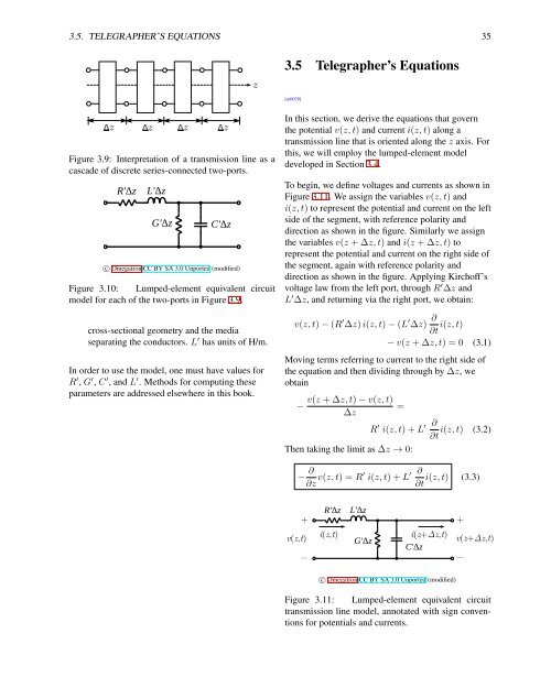
To begin, we define voltages and currents as shown in
Figure 3.11. We assign the variables v(z,t) and
i(z,t) to represent the potential and current on the left
side of the segment, with reference polarity and
direction as shown in the figure. Similarly we assign
the variables v(z +∆z,t) and i(z +∆z,t) to
represent the potential and current on the right side of
the segment, again with reference polarity and
direction as shown in the figure. Applying Kirchoff’s
voltage law from the left port, through R ′ ∆z and
L ′ ∆z, and returning via the right port, we obtain:
v(z,t)−(R ′ ∆z)i(z,t)−(L ′ ∆z) ∂ ∂t i(z,t)
−v(z +∆z,t) = 0 (3.1)
Moving terms referring to current to the right side of
the equation and then dividing through by ∆z, we
obtain
v(z +∆z,t)−v(z,t)
− =
∆z
R ′ i(z,t)+L ′ ∂
i(z,t) (3.2)
∂t
Then taking the limit as∆z → 0:
− ∂ ∂z v(z,t) = R′ i(z,t)+L ′ ∂
i(z,t) (3.3)
∂t
+
R'Δz
L'Δz
+
v(z,t)
_
i(z,t)
G'Δz
i(z+Δz,t)
C'Δz
v(z+Δz,t)
_
c○ Omegatron CC BY SA 3.0 Unported (modified)
Figure 3.11: Lumped-element equivalent circuit
transmission line model, annotated with sign conventions
for potentials and currents.