

Variational Principles in Classical Mechanics - Revised Second Edition, 2019
Variational Principles in Classical Mechanics - Revised Second Edition, 2019
Variational Principles in Classical Mechanics - Revised Second Edition, 2019

Create successful ePaper yourself
Turn your PDF publications into a flip-book with our unique Google optimized e-Paper software.
VARIATIONAL PRINCIPLES<br />
IN<br />
CLASSICAL MECHANICS<br />
REVISED SECOND EDITION<br />
Douglas Cl<strong>in</strong>e<br />
University of Rochester<br />
15 January <strong>2019</strong>
ii<br />
c°<strong>2019</strong>, 2017 by Douglas Cl<strong>in</strong>e<br />
ISBN: 978-0-9988372-8-4 e-book (Adobe PDF)<br />
ISBN: 978-0-9988372-2-2 e-book (K<strong>in</strong>dle)<br />
ISBN: 978-0-9988372-9-1 pr<strong>in</strong>t (Paperback)<br />
<strong>Variational</strong> <strong>Pr<strong>in</strong>ciples</strong> <strong>in</strong> <strong>Classical</strong> <strong>Mechanics</strong>, <strong>Revised</strong> 2 edition<br />
Contributors<br />
Author: Douglas Cl<strong>in</strong>e<br />
Illustrator: Meghan Sarkis<br />
Published by University of Rochester River Campus Libraries<br />
University of Rochester<br />
Rochester, NY 14627<br />
<strong>Variational</strong> <strong>Pr<strong>in</strong>ciples</strong> <strong>in</strong> <strong>Classical</strong> <strong>Mechanics</strong>, <strong>Revised</strong> 2 edition by Douglas Cl<strong>in</strong>e is licensed under a<br />
Creative Commons Attribution-NonCommercial-ShareAlike 4.0 International License (CC BY-NC-SA 4.0),<br />
except where otherwise noted.<br />
You are free to:<br />
• Share — copy or redistribute the material <strong>in</strong> any medium or format.<br />
• Adapt — remix, transform, and build upon the material.<br />
Under the follow<strong>in</strong>g terms:<br />
• Attribution — You must give appropriate credit, provide a l<strong>in</strong>k to the license, and <strong>in</strong>dicate if changes<br />
were made. You must do so <strong>in</strong> any reasonable manner, but not <strong>in</strong> any way that suggests the licensor<br />
endorsesyouoryouruse.<br />
• NonCommercial — You may not use the material for commercial purposes.<br />
• ShareAlike — If you remix, transform, or build upon the material, you must distribute your contributions<br />
under the same license as the orig<strong>in</strong>al.<br />
• No additional restrictions — You may not apply legal terms or technological measures that legally<br />
restrict others from do<strong>in</strong>g anyth<strong>in</strong>g the license permits.<br />
Thelicensorcannotrevokethesefreedomsaslongasyoufollowthelicenseterms.<br />
Version 2.1
Contents<br />
Contents<br />
Preface<br />
Prologue<br />
iii<br />
xvii<br />
xix<br />
1 A brief history of classical mechanics 1<br />
1.1 Introduction.............................................. 1<br />
1.2 Greekantiquity............................................ 1<br />
1.3 MiddleAges.............................................. 2<br />
1.4 AgeofEnlightenment ........................................ 2<br />
1.5 <strong>Variational</strong>methods<strong>in</strong>physics ................................... 5<br />
1.6 The 20 centuryrevolution<strong>in</strong>physics............................... 7<br />
2 ReviewofNewtonianmechanics 9<br />
2.1 Introduction.............................................. 9<br />
2.2 Newton’sLawsofmotion ...................................... 9<br />
2.3 Inertialframesofreference...................................... 10<br />
2.4 First-order<strong>in</strong>tegrals<strong>in</strong>Newtonianmechanics ........................... 11<br />
2.4.1 L<strong>in</strong>earMomentum ...................................... 11<br />
2.4.2 Angularmomentum ..................................... 11<br />
2.4.3 K<strong>in</strong>eticenergy ........................................ 12<br />
2.5 Conservationlaws<strong>in</strong>classicalmechanics.............................. 12<br />
2.6 Motion of f<strong>in</strong>ite-sizedandmany-bodysystems........................... 12<br />
2.7 Centerofmassofamany-bodysystem............................... 13<br />
2.8 Totall<strong>in</strong>earmomentumofamany-bodysystem.......................... 14<br />
2.8.1 Center-of-massdecomposition................................ 14<br />
2.8.2 Equationsofmotion ..................................... 14<br />
2.9 Angularmomentumofamany-bodysystem............................ 16<br />
2.9.1 Center-of-massdecomposition................................ 16<br />
2.9.2 Equationsofmotion ..................................... 16<br />
2.10Workandk<strong>in</strong>eticenergyforamany-bodysystem......................... 18<br />
2.10.1 Center-of-massk<strong>in</strong>eticenergy................................ 18<br />
2.10.2 Conservativeforcesandpotentialenergy.......................... 18<br />
2.10.3 Totalmechanicalenergy................................... 19<br />
2.10.4 Totalmechanicalenergyforconservativesystems..................... 20<br />
2.11VirialTheorem ............................................ 22<br />
2.12ApplicationsofNewton’sequationsofmotion........................... 24<br />
2.12.1 Constantforceproblems................................... 24<br />
2.12.2 L<strong>in</strong>earRestor<strong>in</strong>gForce.................................... 25<br />
2.12.3 Position-dependentconservativeforces........................... 25<br />
2.12.4 Constra<strong>in</strong>edmotion ..................................... 27<br />
2.12.5 VelocityDependentForces.................................. 28<br />
2.12.6 SystemswithVariableMass................................. 29<br />
2.12.7 Rigid-body rotation about a body-fixedrotationaxis................... 31<br />
iii
iv<br />
CONTENTS<br />
2.12.8 Timedependentforces.................................... 34<br />
2.13Solutionofmany-bodyequationsofmotion ............................ 37<br />
2.13.1 Analyticsolution....................................... 37<br />
2.13.2 Successiveapproximation .................................. 37<br />
2.13.3 Perturbationmethod..................................... 37<br />
2.14Newton’sLawofGravitation .................................... 38<br />
2.14.1 Gravitationaland<strong>in</strong>ertialmass............................... 38<br />
2.14.2 Gravitational potential energy .............................. 39<br />
2.14.3 Gravitational potential .................................. 40<br />
2.14.4 Potentialtheory ....................................... 41<br />
2.14.5 Curl of the gravitational field................................ 41<br />
2.14.6 Gauss’sLawforGravitation................................. 43<br />
2.14.7 CondensedformsofNewton’sLawofGravitation..................... 44<br />
2.15Summary ............................................... 46<br />
Problems .................................................. 48<br />
3 L<strong>in</strong>ear oscillators 51<br />
3.1 Introduction.............................................. 51<br />
3.2 L<strong>in</strong>earrestor<strong>in</strong>gforces ........................................ 51<br />
3.3 L<strong>in</strong>earityandsuperposition ..................................... 52<br />
3.4 Geometricalrepresentationsofdynamicalmotion......................... 53<br />
3.4.1 Configuration space ( ) ................................ 53<br />
3.4.2 State space, ( ˙ ) ..................................... 54<br />
3.4.3 Phase space, ( ) .................................... 54<br />
3.4.4 Planependulum ....................................... 55<br />
3.5 L<strong>in</strong>early-damped free l<strong>in</strong>ear oscillator ................................ 56<br />
3.5.1 Generalsolution ....................................... 56<br />
3.5.2 Energydissipation ...................................... 59<br />
3.6 S<strong>in</strong>usoidally-drive, l<strong>in</strong>early-damped, l<strong>in</strong>ear oscillator . . . .................... 60<br />
3.6.1 Transient response of a driven oscillator .......................... 60<br />
3.6.2 Steady state response of a driven oscillator ........................ 61<br />
3.6.3 Completesolutionofthedrivenoscillator ......................... 62<br />
3.6.4 Resonance........................................... 63<br />
3.6.5 Energyabsorption ...................................... 63<br />
3.7 Waveequation ............................................ 66<br />
3.8 Travell<strong>in</strong>gandstand<strong>in</strong>gwavesolutionsofthewaveequation................... 67<br />
3.9 Waveformanalysis .......................................... 68<br />
3.9.1 Harmonicdecomposition................................... 68<br />
3.9.2 The free l<strong>in</strong>early-damped l<strong>in</strong>ear oscillator ......................... 68<br />
3.9.3 Dampedl<strong>in</strong>earoscillatorsubjecttoanarbitraryperiodicforce ............. 69<br />
3.10Signalprocess<strong>in</strong>g ........................................... 70<br />
3.11 Wave propagation .......................................... 71<br />
3.11.1 Phase,group,andsignalvelocitiesofwavepackets .................... 72<br />
3.11.2 Fouriertransformofwavepackets ............................. 77<br />
3.11.3 Wave-packetUncerta<strong>in</strong>tyPr<strong>in</strong>ciple............................. 78<br />
3.12Summary ............................................... 80<br />
Problems .................................................. 83<br />
4 Nonl<strong>in</strong>ear systems and chaos 85<br />
4.1 Introduction.............................................. 85<br />
4.2 Weaknonl<strong>in</strong>earity .......................................... 86<br />
4.3 Bifurcation,andpo<strong>in</strong>tattractors .................................. 88<br />
4.4 Limitcycles.............................................. 89<br />
4.4.1 Po<strong>in</strong>caré-Bendixsontheorem ................................ 89<br />
4.4.2 vanderPoldampedharmonicoscillator:.......................... 90
CONTENTS<br />
v<br />
4.5 Harmonically-driven,l<strong>in</strong>early-damped,planependulum...................... 93<br />
4.5.1 Closetol<strong>in</strong>earity....................................... 93<br />
4.5.2 Weaknonl<strong>in</strong>earity ...................................... 95<br />
4.5.3 Onsetofcomplication .................................... 96<br />
4.5.4 Perioddoubl<strong>in</strong>gandbifurcation............................... 96<br />
4.5.5 Roll<strong>in</strong>g motion ........................................ 96<br />
4.5.6 Onsetofchaos ........................................ 97<br />
4.6 Differentiationbetweenorderedandchaoticmotion........................ 98<br />
4.6.1 Lyapunovexponent ..................................... 98<br />
4.6.2 Bifurcationdiagram ..................................... 99<br />
4.6.3 Po<strong>in</strong>caréSection .......................................100<br />
4.7 Wave propagation for non-l<strong>in</strong>ear systems . . . ...........................101<br />
4.7.1 Phase,group,andsignalvelocities .............................101<br />
4.7.2 Soliton wave propagation ..................................103<br />
4.8 Summary ...............................................104<br />
Problems ..................................................106<br />
5 Calculus of variations 107<br />
5.1 Introduction..............................................107<br />
5.2 Euler’s differentialequation .....................................108<br />
5.3 ApplicationsofEuler’sequation...................................110<br />
5.4 Selectionofthe<strong>in</strong>dependentvariable................................113<br />
5.5 Functions with several <strong>in</strong>dependent variables () ........................115<br />
5.6 Euler’s<strong>in</strong>tegralequation.......................................117<br />
5.7 Constra<strong>in</strong>edvariationalsystems...................................118<br />
5.7.1 Holonomicconstra<strong>in</strong>ts....................................118<br />
5.7.2 Geometric(algebraic)equationsofconstra<strong>in</strong>t .......................118<br />
5.7.3 K<strong>in</strong>ematic (differential)equationsofconstra<strong>in</strong>t ......................118<br />
5.7.4 Isoperimetric(<strong>in</strong>tegral)equationsofconstra<strong>in</strong>t ......................119<br />
5.7.5 Propertiesoftheconstra<strong>in</strong>tequations ...........................119<br />
5.7.6 Treatmentofconstra<strong>in</strong>tforces<strong>in</strong>variationalcalculus...................120<br />
5.8 Generalizedcoord<strong>in</strong>ates<strong>in</strong>variationalcalculus ..........................121<br />
5.9 Lagrangemultipliersforholonomicconstra<strong>in</strong>ts ..........................122<br />
5.9.1 Algebraicequationsofconstra<strong>in</strong>t..............................122<br />
5.9.2 Integralequationsofconstra<strong>in</strong>t...............................124<br />
5.10Geodesic................................................126<br />
5.11<strong>Variational</strong>approachtoclassicalmechanics ............................127<br />
5.12Summary ...............................................128<br />
Problems ..................................................129<br />
6 Lagrangian dynamics 131<br />
6.1 Introduction..............................................131<br />
6.2 Newtonian plausibility argument for Lagrangian mechanics ...................132<br />
6.3 Lagrangeequationsfromd’Alembert’sPr<strong>in</strong>ciple..........................134<br />
6.3.1 d’Alembert’sPr<strong>in</strong>cipleofVirtualWork ..........................134<br />
6.3.2 Transformationtogeneralizedcoord<strong>in</strong>ates.........................135<br />
6.3.3 Lagrangian ..........................................136<br />
6.4 LagrangeequationsfromHamilton’sActionPr<strong>in</strong>ciple ......................137<br />
6.5 Constra<strong>in</strong>edsystems .........................................138<br />
6.5.1 Choiceofgeneralizedcoord<strong>in</strong>ates..............................138<br />
6.5.2 M<strong>in</strong>imalsetofgeneralizedcoord<strong>in</strong>ates...........................138<br />
6.5.3 Lagrangemultipliersapproach ...............................138<br />
6.5.4 Generalizedforcesapproach.................................140<br />
6.6 Apply<strong>in</strong>gtheEuler-Lagrangeequationstoclassicalmechanics..................140<br />
6.7 Applicationstounconstra<strong>in</strong>edsystems...............................142
vi<br />
CONTENTS<br />
6.8 Applicationstosystems<strong>in</strong>volv<strong>in</strong>gholonomicconstra<strong>in</strong>ts .....................144<br />
6.9 Applications<strong>in</strong>volv<strong>in</strong>gnon-holonomicconstra<strong>in</strong>ts.........................157<br />
6.10Velocity-dependentLorentzforce ..................................164<br />
6.11Time-dependentforces........................................165<br />
6.12Impulsiveforces............................................166<br />
6.13TheLagrangianversustheNewtonianapproachtoclassicalmechanics.............168<br />
6.14Summary ...............................................169<br />
Problems ..................................................172<br />
7 Symmetries, Invariance and the Hamiltonian 175<br />
7.1 Introduction..............................................175<br />
7.2 Generalizedmomentum .......................................175<br />
7.3 InvarianttransformationsandNoether’sTheorem.........................177<br />
7.4 Rotational<strong>in</strong>varianceandconservationofangularmomentum..................179<br />
7.5 Cycliccoord<strong>in</strong>ates ..........................................180<br />
7.6 K<strong>in</strong>eticenergy<strong>in</strong>generalizedcoord<strong>in</strong>ates .............................181<br />
7.7 GeneralizedenergyandtheHamiltonianfunction.........................182<br />
7.8 Generalizedenergytheorem.....................................183<br />
7.9 Generalizedenergyandtotalenergy ................................183<br />
7.10Hamiltonian<strong>in</strong>variance........................................184<br />
7.11Hamiltonianforcycliccoord<strong>in</strong>ates .................................189<br />
7.12Symmetriesand<strong>in</strong>variance .....................................189<br />
7.13Hamiltonian<strong>in</strong>classicalmechanics .................................189<br />
7.14Summary ...............................................190<br />
Problems ..................................................192<br />
8 Hamiltonian mechanics 195<br />
8.1 Introduction..............................................195<br />
8.2 LegendreTransformationbetweenLagrangianandHamiltonianmechanics...........196<br />
8.3 Hamilton’sequationsofmotion...................................197<br />
8.3.1 Canonicalequationsofmotion ...............................198<br />
8.4 Hamiltonian <strong>in</strong> differentcoord<strong>in</strong>atesystems............................199<br />
8.4.1 Cyl<strong>in</strong>drical coord<strong>in</strong>ates ................................199<br />
8.4.2 Spherical coord<strong>in</strong>ates, .................................200<br />
8.5 ApplicationsofHamiltonianDynamics...............................201<br />
8.6 Routhianreduction..........................................206<br />
8.6.1 R -RouthianisaHamiltonianforthecyclicvariables................207<br />
8.6.2 R -RouthianisaHamiltonianforthenon-cyclicvariables ...........208<br />
8.7 Variable-masssystems ........................................212<br />
8.7.1 Rocketpropulsion:......................................212<br />
8.7.2 Mov<strong>in</strong>gcha<strong>in</strong>s: ........................................213<br />
8.8 Summary ...............................................215<br />
Problems ..................................................217<br />
9 Hamilton’s Action Pr<strong>in</strong>ciple 221<br />
9.1 Introduction..............................................221<br />
9.2 Hamilton’s Pr<strong>in</strong>ciple of Stationary Action<br />
9.2.1 Stationary-actionpr<strong>in</strong>ciple<strong>in</strong>Lagrangianmechanics ...................222<br />
9.2.2 Stationary-actionpr<strong>in</strong>ciple<strong>in</strong>Hamiltonianmechanics ..................223<br />
9.2.3 Abbreviatedaction......................................224<br />
9.2.4 Hamilton’s Pr<strong>in</strong>ciple applied us<strong>in</strong>g <strong>in</strong>itial boundary conditions . ............225<br />
9.3 Lagrangian ..............................................228<br />
9.3.1 StandardLagrangian.....................................228<br />
9.3.2 Gauge<strong>in</strong>varianceofthestandardLagrangian .......................228<br />
9.3.3 Non-standardLagrangians..................................230<br />
9.3.4 Inversevariationalcalculus .................................230
CONTENTS<br />
vii<br />
9.4 ApplicationofHamilton’sActionPr<strong>in</strong>cipletomechanics.....................231<br />
9.5 Summary ...............................................232<br />
10 Nonconservative systems 235<br />
10.1Introduction..............................................235<br />
10.2Orig<strong>in</strong>sofnonconservativemotion .................................235<br />
10.3Algebraicmechanicsfornonconservativesystems .........................236<br />
10.4Rayleigh’sdissipationfunction ...................................236<br />
10.4.1 Generalizeddissipativeforcesforl<strong>in</strong>earvelocitydependence...............237<br />
10.4.2 Generalizeddissipativeforcesfornonl<strong>in</strong>earvelocitydependence.............238<br />
10.4.3 Lagrangeequationsofmotion................................238<br />
10.4.4 Hamiltonianmechanics ...................................238<br />
10.5DissipativeLagrangians .......................................241<br />
10.6Summary ...............................................243<br />
11 Conservative two-body central forces 245<br />
11.1Introduction..............................................245<br />
11.2Equivalentone-bodyrepresentationfortwo-bodymotion.....................246<br />
11.3 Angular momentum L ........................................248<br />
11.4Equationsofmotion .........................................249<br />
11.5 Differentialorbitequation:......................................250<br />
11.6Hamiltonian..............................................251<br />
11.7Generalfeaturesoftheorbitsolutions ...............................252<br />
11.8Inverse-square,two-body,centralforce...............................253<br />
11.8.1 Boundorbits .........................................254<br />
11.8.2 Kepler’slawsforboundplanetarymotion .........................255<br />
11.8.3 Unboundorbits........................................256<br />
11.8.4 Eccentricity vector . . . ...................................257<br />
11.9Isotropic,l<strong>in</strong>ear,two-body,centralforce ..............................259<br />
11.9.1 Polarcoord<strong>in</strong>ates.......................................260<br />
11.9.2 Cartesiancoord<strong>in</strong>ates ....................................261<br />
11.9.3 Symmetry tensor A 0 .....................................262<br />
11.10Closed-orbitstability.........................................263<br />
11.11Thethree-bodyproblem.......................................268<br />
11.12Two-bodyscatter<strong>in</strong>g.........................................269<br />
11.12.1Totaltwo-bodyscatter<strong>in</strong>gcrosssection ..........................269<br />
11.12.2 Differentialtwo-bodyscatter<strong>in</strong>gcrosssection .......................270<br />
11.12.3Impactparameterdependenceonscatter<strong>in</strong>gangle ....................270<br />
11.12.4Rutherfordscatter<strong>in</strong>g ....................................272<br />
11.13Two-bodyk<strong>in</strong>ematics.........................................274<br />
11.14Summary ...............................................280<br />
Problems ..................................................282<br />
12 Non-<strong>in</strong>ertial reference frames 285<br />
12.1Introduction..............................................285<br />
12.2 Translational acceleration of a reference frame ...........................285<br />
12.3Rotat<strong>in</strong>greferenceframe.......................................286<br />
12.3.1 Spatialtimederivatives<strong>in</strong>arotat<strong>in</strong>g,non-translat<strong>in</strong>g,referenceframe .........286<br />
12.3.2 Generalvector<strong>in</strong>arotat<strong>in</strong>g,non-translat<strong>in</strong>g,referenceframe ..............287<br />
12.4 Reference frame undergo<strong>in</strong>g rotation plus translation . . . ....................288<br />
12.5Newton’slawofmotion<strong>in</strong>anon-<strong>in</strong>ertialframe ..........................288<br />
12.6Lagrangianmechanics<strong>in</strong>anon-<strong>in</strong>ertialframe ...........................289<br />
12.7Centrifugalforce ...........................................290<br />
12.8Coriolisforce .............................................291<br />
12.9Routhianreductionforrotat<strong>in</strong>gsystems ..............................295<br />
12.10EffectivegravitationalforcenearthesurfaceoftheEarth ....................298
viii<br />
CONTENTS<br />
12.11Freemotionontheearth.......................................300<br />
12.12Weathersystems ...........................................302<br />
12.12.1Low-pressuresystems: ....................................302<br />
12.12.2High-pressuresystems:....................................304<br />
12.13Foucaultpendulum..........................................304<br />
12.14Summary ...............................................306<br />
Problems ..................................................307<br />
13 Rigid-body rotation 309<br />
13.1Introduction..............................................309<br />
13.2Rigid-bodycoord<strong>in</strong>ates........................................310<br />
13.3 Rigid-body rotation about a body-fixedpo<strong>in</strong>t...........................310<br />
13.4Inertiatensor .............................................312<br />
13.5Matrixandtensorformulationsofrigid-bodyrotation ......................313<br />
13.6Pr<strong>in</strong>cipalaxissystem.........................................313<br />
13.7 Diagonalize the <strong>in</strong>ertia tensor . ...................................314<br />
13.8Parallel-axistheorem.........................................315<br />
13.9Perpendicular-axistheoremforplanelam<strong>in</strong>ae ...........................318<br />
13.10Generalpropertiesofthe<strong>in</strong>ertiatensor...............................319<br />
13.10.1Inertialequivalence......................................319<br />
13.10.2 Orthogonality of pr<strong>in</strong>cipal axes ...............................320<br />
13.11Angular momentum L and angular velocity ω vectors ......................321<br />
13.12K<strong>in</strong>eticenergyofrotat<strong>in</strong>grigidbody................................323<br />
13.13Eulerangles..............................................325<br />
13.14Angular velocity ω ..........................................327<br />
13.15K<strong>in</strong>eticenergy<strong>in</strong>termsofEulerangularvelocities ........................328<br />
13.16Rotational<strong>in</strong>variants.........................................329<br />
13.17Euler’sequationsofmotionforrigid-bodyrotation ........................330<br />
13.18Lagrangeequationsofmotionforrigid-bodyrotation.......................331<br />
13.19Hamiltonianequationsofmotionforrigid-bodyrotation.....................333<br />
13.20Torque-freerotationofan<strong>in</strong>ertially-symmetricrigidrotor ....................333<br />
13.20.1Euler’sequationsofmotion:.................................333<br />
13.20.2Lagrangeequationsofmotion: ...............................337<br />
13.21Torque-freerotationofanasymmetricrigidrotor.........................339<br />
13.22Stability of torque-free rotation of an asymmetric body . . ....................340<br />
13.23Symmetric rigid rotor subject to torque about a fixedpo<strong>in</strong>t ...................343<br />
13.24Theroll<strong>in</strong>gwheel...........................................347<br />
13.25Dynamicbalanc<strong>in</strong>gofwheels ....................................350<br />
13.26Rotationofdeformablebodies....................................351<br />
13.27Summary ...............................................352<br />
Problems ..................................................354<br />
14 Coupled l<strong>in</strong>ear oscillators 357<br />
14.1Introduction..............................................357<br />
14.2 Two coupled l<strong>in</strong>ear oscillators . ...................................357<br />
14.3Normalmodes ............................................359<br />
14.4 Center of mass oscillations . . . ...................................360<br />
14.5Weakcoupl<strong>in</strong>g ............................................361<br />
14.6Generalanalytictheoryforcoupledl<strong>in</strong>earoscillators .......................363<br />
14.6.1 K<strong>in</strong>etic energy tensor T ...................................363<br />
14.6.2 Potential energy tensor V ..................................364<br />
14.6.3 Equationsofmotion .....................................365<br />
14.6.4 Superposition.........................................366<br />
14.6.5 Eigenfunctionorthonormality................................366<br />
14.6.6 Normalcoord<strong>in</strong>ates .....................................367
CONTENTS<br />
ix<br />
14.7 Two-body coupled oscillator systems ................................368<br />
14.8 Three-body coupled l<strong>in</strong>ear oscillator systems . ...........................374<br />
14.9Molecularcoupledoscillatorsystems ................................379<br />
14.10DiscreteLatticeCha<strong>in</strong>........................................382<br />
14.10.1Longitud<strong>in</strong>almotion.....................................382<br />
14.10.2Transversemotion ......................................382<br />
14.10.3Normalmodes........................................383<br />
14.10.4 Travell<strong>in</strong>g waves .......................................386<br />
14.10.5Dispersion...........................................386<br />
14.10.6Complexwavenumber ....................................387<br />
14.11Damped coupled l<strong>in</strong>ear oscillators ..................................388<br />
14.12Collective synchronization of coupled oscillators ..........................389<br />
14.13Summary ...............................................392<br />
Problems ..................................................393<br />
15 Advanced Hamiltonian mechanics 395<br />
15.1Introduction..............................................395<br />
15.2PoissonbracketrepresentationofHamiltonianmechanics ....................397<br />
15.2.1 PoissonBrackets .......................................397<br />
15.2.2 FundamentalPoissonbrackets: ...............................397<br />
15.2.3 Poissonbracket<strong>in</strong>variancetocanonicaltransformations .................398<br />
15.2.4 CorrespondenceofthecommutatorandthePoissonBracket...............399<br />
15.2.5 Observables<strong>in</strong>Hamiltonianmechanics...........................400<br />
15.2.6 Hamilton’sequationsofmotion...............................403<br />
15.2.7 Liouville’s Theorem . . ...................................407<br />
15.3Canonicaltransformations<strong>in</strong>Hamiltonianmechanics.......................409<br />
15.3.1 Generat<strong>in</strong>gfunctions.....................................410<br />
15.3.2 Applicationsofcanonicaltransformations .........................412<br />
15.4Hamilton-Jacobitheory .......................................414<br />
15.4.1 Time-dependentHamiltonian................................414<br />
15.4.2 Time-<strong>in</strong>dependentHamiltonian...............................416<br />
15.4.3 Separationofvariables....................................417<br />
15.4.4 Visual representation of the action function . ......................424<br />
15.4.5 AdvantagesofHamilton-Jacobitheory...........................424<br />
15.5Action-anglevariables ........................................425<br />
15.5.1 Canonicaltransformation ..................................425<br />
15.5.2 Adiabatic<strong>in</strong>varianceoftheactionvariables ........................428<br />
15.6Canonicalperturbationtheory ...................................430<br />
15.7Symplecticrepresentation ......................................432<br />
15.8ComparisonoftheLagrangianandHamiltonianformulations ..................432<br />
15.9Summary ...............................................434<br />
Problems ..................................................437<br />
16 Analytical formulations for cont<strong>in</strong>uous systems 439<br />
16.1Introduction..............................................439<br />
16.2Thecont<strong>in</strong>uousuniforml<strong>in</strong>earcha<strong>in</strong> ................................439<br />
16.3TheLagrangiandensityformulationforcont<strong>in</strong>uoussystems ...................440<br />
16.3.1 Onespatialdimension....................................440<br />
16.3.2 Threespatialdimensions ..................................441<br />
16.4TheHamiltoniandensityformulationforcont<strong>in</strong>uoussystems ..................442<br />
16.5L<strong>in</strong>earelasticsolids..........................................443<br />
16.5.1 Stresstensor .........................................444<br />
16.5.2 Stra<strong>in</strong>tensor .........................................444<br />
16.5.3 Moduliofelasticity......................................445<br />
16.5.4 Equationsofmotion<strong>in</strong>auniformelasticmedia......................446
x<br />
CONTENTS<br />
16.6 Electromagnetic fieldtheory.....................................447<br />
16.6.1 Maxwellstresstensor ....................................447<br />
16.6.2 Momentum <strong>in</strong> the electromagnetic field ..........................448<br />
16.7 Ideal fluiddynamics .........................................449<br />
16.7.1 Cont<strong>in</strong>uityequation .....................................449<br />
16.7.2 Euler’shydrodynamicequation...............................449<br />
16.7.3 Irrotational flow and Bernoulli’s equation .........................450<br />
16.7.4 Gas flow............................................450<br />
16.8 Viscous fluiddynamics........................................452<br />
16.8.1 Navier-Stokesequation....................................452<br />
16.8.2 Reynoldsnumber.......................................453<br />
16.8.3 Lam<strong>in</strong>ar and turbulent fluid flow..............................453<br />
16.9Summaryandimplications .....................................455<br />
17 Relativistic mechanics 457<br />
17.1Introduction..............................................457<br />
17.2GalileanInvariance..........................................457<br />
17.3SpecialTheoryofRelativity.....................................459<br />
17.3.1 E<strong>in</strong>ste<strong>in</strong>Postulates......................................459<br />
17.3.2 Lorentztransformation ...................................459<br />
17.3.3 TimeDilation: ........................................460<br />
17.3.4 LengthContraction .....................................461<br />
17.3.5 Simultaneity .........................................461<br />
17.4Relativistick<strong>in</strong>ematics........................................464<br />
17.4.1 Velocitytransformations...................................464<br />
17.4.2 Momentum ..........................................464<br />
17.4.3 Centerofmomentumcoord<strong>in</strong>atesystem..........................465<br />
17.4.4 Force .............................................465<br />
17.4.5 Energy.............................................465<br />
17.5Geometryofspace-time .......................................467<br />
17.5.1 Four-dimensionalspace-time ................................467<br />
17.5.2 Four-vectorscalarproducts .................................468<br />
17.5.3 M<strong>in</strong>kowskispace-time ....................................469<br />
17.5.4 Momentum-energyfourvector ...............................470<br />
17.6Lorentz-<strong>in</strong>variantformulationofLagrangianmechanics......................471<br />
17.6.1 Parametricformulation ...................................471<br />
17.6.2 ExtendedLagrangian ....................................471<br />
17.6.3 Extendedgeneralizedmomenta...............................473<br />
17.6.4 ExtendedLagrangeequationsofmotion ..........................473<br />
17.7Lorentz-<strong>in</strong>variantformulationsofHamiltonianmechanics.....................476<br />
17.7.1 Extendedcanonicalformalism................................476<br />
17.7.2 ExtendedPoissonBracketrepresentation .........................478<br />
17.7.3 ExtendedcanonicaltransformationandHamilton-Jacobitheory.............478<br />
17.7.4 ValidityoftheextendedHamilton-Lagrangeformalism..................478<br />
17.8TheGeneralTheoryofRelativity..................................480<br />
17.8.1 Thefundamentalconcepts..................................480<br />
17.8.2 E<strong>in</strong>ste<strong>in</strong>’spostulatesfortheGeneralTheoryofRelativity ................481<br />
17.8.3 Experimentalevidence<strong>in</strong>supportoftheGeneralTheoryofRelativity .........481<br />
17.9Implicationsofrelativistictheorytoclassicalmechanics .....................482<br />
17.10Summary ...............................................483<br />
Problems ..................................................484<br />
18 The transition to quantum physics 485<br />
18.1Introduction..............................................485<br />
18.2Briefsummaryoftheorig<strong>in</strong>sofquantumtheory .........................485
CONTENTS<br />
xi<br />
18.2.1 Bohrmodeloftheatom...................................487<br />
18.2.2 Quantization .........................................487<br />
18.2.3 Wave-particleduality ....................................488<br />
18.3Hamiltonian<strong>in</strong>quantumtheory...................................489<br />
18.3.1 Heisenberg’smatrix-mechanicsrepresentation.......................489<br />
18.3.2 Schröd<strong>in</strong>ger’swave-mechanicsrepresentation .......................491<br />
18.4Lagrangianrepresentation<strong>in</strong>quantumtheory...........................492<br />
18.5CorrespondencePr<strong>in</strong>ciple ......................................493<br />
18.6Summary ...............................................494<br />
19 Epilogue 495<br />
Appendices<br />
A Matrix algebra 497<br />
A.1 Mathematicalmethodsformechanics................................497<br />
A.2 Matrices................................................497<br />
A.3 Determ<strong>in</strong>ants .............................................501<br />
A.4 Reduction of a matrix to diagonal form . . . ...........................503<br />
B Vector algebra 505<br />
B.1 L<strong>in</strong>earoperations...........................................505<br />
B.2 Scalarproduct ............................................505<br />
B.3 Vectorproduct ............................................506<br />
B.4 Tripleproducts............................................507<br />
C Orthogonal coord<strong>in</strong>ate systems 509<br />
C.1 Cartesian coord<strong>in</strong>ates ( ) ....................................509<br />
C.2 Curvil<strong>in</strong>ear coord<strong>in</strong>ate systems ...................................509<br />
C.2.1 Two-dimensional polar coord<strong>in</strong>ates ( ) ..........................510<br />
C.2.2 Cyl<strong>in</strong>drical Coord<strong>in</strong>ates ( ) ..............................512<br />
C.2.3 Spherical Coord<strong>in</strong>ates ( ) ................................512<br />
C.3 Frenet-Serretcoord<strong>in</strong>ates ......................................513<br />
D Coord<strong>in</strong>ate transformations 515<br />
D.1 Translationaltransformations....................................515<br />
D.2 Rotationaltransformations .....................................515<br />
D.2.1 Rotationmatrix .......................................515<br />
D.2.2 F<strong>in</strong>iterotations........................................518<br />
D.2.3 Inf<strong>in</strong>itessimalrotations....................................519<br />
D.2.4 Properandimproperrotations ...............................519<br />
D.3 Spatial<strong>in</strong>versiontransformation...................................520<br />
D.4 Timereversaltransformation ....................................521<br />
E Tensor algebra 523<br />
E.1 Tensors ................................................523<br />
E.2 Tensorproducts............................................524<br />
E.2.1 Tensorouterproduct.....................................524<br />
E.2.2 Tensor<strong>in</strong>nerproduct.....................................524<br />
E.3 Tensorproperties...........................................525<br />
E.4 Contravariantandcovarianttensors ................................526<br />
E.5 Generalized<strong>in</strong>nerproduct......................................527<br />
E.6 Transformationpropertiesofobservables..............................528<br />
F Aspects of multivariate calculus 529<br />
F.1 Partial differentiation ........................................529
xii<br />
CONTENTS<br />
F.2 L<strong>in</strong>earoperators ...........................................529<br />
F.3 TransformationJacobian.......................................531<br />
F.3.1 Transformationof<strong>in</strong>tegrals:.................................531<br />
F.3.2 Transformation of differentialequations:..........................531<br />
F.3.3 PropertiesoftheJacobian: .................................531<br />
F.4 Legendretransformation.......................................532<br />
G Vector differential calculus 533<br />
G.1 Scalar differentialoperators .....................................533<br />
G.1.1 Scalar field ..........................................533<br />
G.1.2 Vector field ..........................................533<br />
G.2 Vector differentialoperators<strong>in</strong>cartesiancoord<strong>in</strong>ates .......................533<br />
G.2.1 Scalar field ..........................................533<br />
G.2.2 Vector field ..........................................534<br />
G.3 Vector differential operators <strong>in</strong> curvil<strong>in</strong>ear coord<strong>in</strong>ates . . ....................535<br />
G.3.1 Gradient: ...........................................535<br />
G.3.2 Divergence: ..........................................536<br />
G.3.3 Curl:..............................................536<br />
G.3.4 Laplacian:...........................................536<br />
H Vector <strong>in</strong>tegral calculus 537<br />
H.1 L<strong>in</strong>e <strong>in</strong>tegral of the gradient of a scalar field............................537<br />
H.2 Divergencetheorem .........................................537<br />
H.2.1 Flux of a vector fieldforGaussiansurface.........................537<br />
H.2.2 Divergence<strong>in</strong>cartesiancoord<strong>in</strong>ates. ............................538<br />
H.3 StokesTheorem............................................540<br />
H.3.1 Thecurl............................................540<br />
H.3.2 Curl<strong>in</strong>cartesiancoord<strong>in</strong>ates................................541<br />
H.4 Potential formulations of curl-free and divergence-free fields ...................543<br />
I Waveform analysis 545<br />
I.1 Harmonicwaveformdecomposition.................................545<br />
I.1.1 PeriodicsystemsandtheFourierseries...........................545<br />
I.1.2 AperiodicsystemsandtheFourierTransform.......................547<br />
I.2 Time-sampledwaveformanalysis ..................................548<br />
I.2.1 Delta-functionimpulseresponse ..............................549<br />
I.2.2 Green’sfunctionwaveformdecomposition .........................550<br />
Bibliography 551<br />
Index 555
Examples<br />
2.1 Example: Explod<strong>in</strong>g cannon shell .................................... 15<br />
2.2 Example: Billiard-ball collisions ..................................... 15<br />
2.3 Example: Bolas thrown by gaucho ................................... 17<br />
2.4 Example: Central force ......................................... 20<br />
2.5 Example: The ideal gas law ....................................... 23<br />
2.6 Example: The mass of galaxies ..................................... 23<br />
2.7 Example: Diatomic molecule ...................................... 26<br />
2.8 Example: Roller coaster ......................................... 27<br />
2.9 Example: Vertical fall <strong>in</strong> the earth’s gravitational field. ........................ 28<br />
2.10 Example: Projectile motion <strong>in</strong> air ................................... 29<br />
2.11 Example: Moment of <strong>in</strong>ertia of a th<strong>in</strong> door .............................. 33<br />
2.12 Example: Merry-go-round ........................................ 33<br />
2.13 Example: Cue pushes a billiard ball .................................. 33<br />
2.14 Example: Center of percussion of a baseball bat ............................ 35<br />
2.15 Example: Energy transfer <strong>in</strong> charged-particle scatter<strong>in</strong>g ....................... 36<br />
2.16 Example: Field of a uniform sphere .................................. 45<br />
3.1 Example: Harmonically-driven series RLC circuit .......................... 65<br />
3.2 Example: Vibration isolation ...................................... 69<br />
3.3 Example: Water waves break<strong>in</strong>g on a beach .............................. 74<br />
3.4 Example: Surface waves for deep water ................................ 74<br />
3.5 Example: Electromagnetic waves <strong>in</strong> ionosphere ............................ 75<br />
3.6 Example: Fourier transform of a Gaussian wave packet: ....................... 77<br />
3.7 Example: Fourier transform of a rectangular wave packet: ...................... 77<br />
3.8 Example: Acoustic wave packet ..................................... 79<br />
3.9 Example: Gravitational red shift .................................... 79<br />
3.10 Example: Quantum baseball ....................................... 80<br />
4.1 Example: Non-l<strong>in</strong>ear oscillator ..................................... 87<br />
5.1 Example: Shortest distance between two po<strong>in</strong>ts ............................110<br />
5.2 Example: Brachistochrone problem ...................................110<br />
5.3 Example: M<strong>in</strong>imal travel cost ......................................112<br />
5.4 Example: Surface area of a cyl<strong>in</strong>drically-symmetric soap bubble ...................113<br />
5.5 Example: Fermat’s Pr<strong>in</strong>ciple ......................................115<br />
5.6 Example: M<strong>in</strong>imum of (∇) 2 <strong>in</strong> a volume ..............................117<br />
5.7 Example: Two dependent variables coupled by one holonomic constra<strong>in</strong>t ..............123<br />
5.8 Example: Catenary ............................................125<br />
5.9 Example: The Queen Dido problem ...................................125<br />
6.1 Example: Motion of a free particle, U=0 ...............................142<br />
6.2 Example: Motion <strong>in</strong> a uniform gravitational field ...........................142<br />
6.3 Example: Central forces .........................................143<br />
6.4 Example: Disk roll<strong>in</strong>g on an <strong>in</strong>cl<strong>in</strong>ed plane ..............................144<br />
6.5 Example: Two connected masses on frictionless <strong>in</strong>cl<strong>in</strong>ed planes ...................147<br />
6.6 Example: Two blocks connected by a frictionless bar .........................148<br />
6.7 Example: Block slid<strong>in</strong>g on a movable frictionless <strong>in</strong>cl<strong>in</strong>ed plane ...................149<br />
6.8 Example: Sphere roll<strong>in</strong>g without slipp<strong>in</strong>g down an <strong>in</strong>cl<strong>in</strong>ed plane on a frictionless floor. .....150<br />
6.9 Example: Mass slid<strong>in</strong>g on a rotat<strong>in</strong>g straight frictionless rod. ....................150<br />
xiii
xiv<br />
EXAMPLES<br />
6.10 Example: Spherical pendulum ......................................151<br />
6.11 Example: Spr<strong>in</strong>g plane pendulum ....................................152<br />
6.12 Example: The yo-yo ...........................................153<br />
6.13 Example: Mass constra<strong>in</strong>ed to move on the <strong>in</strong>side of a frictionless paraboloid ...........154<br />
6.14 Example: Mass on a frictionless plane connected to a plane pendulum ...............155<br />
6.15 Example: Two connected masses constra<strong>in</strong>ed to slide along a mov<strong>in</strong>g rod ..............156<br />
6.16 Example: Mass slid<strong>in</strong>g on a frictionless spherical shell ........................157<br />
6.17 Example: Roll<strong>in</strong>g solid sphere on a spherical shell ..........................159<br />
6.18 Example: Solid sphere roll<strong>in</strong>g plus slipp<strong>in</strong>g on a spherical shell ...................161<br />
6.19 Example: Small body held by friction on the periphery of a roll<strong>in</strong>g wheel ..............162<br />
6.20 Example: Plane pendulum hang<strong>in</strong>g from a vertically-oscillat<strong>in</strong>g support ..............165<br />
6.21 Example: Series-coupled double pendulum subject to impulsive force .................167<br />
7.1 Example: Feynman’s angular-momentum paradox ...........................176<br />
7.2 Example: Atwoods mach<strong>in</strong>e .......................................178<br />
7.3 Example: Conservation of angular momentum for rotational <strong>in</strong>variance: ..............179<br />
7.4 Example: Diatomic molecules and axially-symmetric nuclei .....................180<br />
7.5 Example: L<strong>in</strong>ear harmonic oscillator on a cart mov<strong>in</strong>g at constant velocity ............185<br />
7.6 Example: Isotropic central force <strong>in</strong> a rotat<strong>in</strong>g frame .........................186<br />
7.7 Example: The plane pendulum .....................................187<br />
7.8 Example: Oscillat<strong>in</strong>g cyl<strong>in</strong>der <strong>in</strong> a cyl<strong>in</strong>drical bowl ..........................187<br />
8.1 Example: Motion <strong>in</strong> a uniform gravitational field ...........................201<br />
8.2 Example: One-dimensional harmonic oscillator ............................201<br />
8.3 Example: Plane pendulum ........................................202<br />
8.4 Example: Hooke’s law force constra<strong>in</strong>ed to the surface of a cyl<strong>in</strong>der .................203<br />
8.5 Example: Electron motion <strong>in</strong> a cyl<strong>in</strong>drical magnetron ........................204<br />
8.6 Example: Spherical pendulum us<strong>in</strong>g Hamiltonian mechanics .....................209<br />
8.7 Example: Spherical pendulum us<strong>in</strong>g ( ˙ ˙ ) .....................210<br />
8.8 Example: Spherical pendulum us<strong>in</strong>g ( ˙) ...................211<br />
8.9 Example: S<strong>in</strong>gle particle mov<strong>in</strong>g <strong>in</strong> a vertical plane under the <strong>in</strong>fluence of an <strong>in</strong>verse-square<br />
central force ...............................................212<br />
8.10 Example: Folded cha<strong>in</strong> ..........................................213<br />
8.11 Example: Fall<strong>in</strong>g cha<strong>in</strong> .........................................214<br />
9.1 Example: Gauge <strong>in</strong>variance <strong>in</strong> electromagnetism ...........................229<br />
10.1 Example: Driven, l<strong>in</strong>early-damped, coupled l<strong>in</strong>ear oscillators .....................239<br />
10.2 Example: Kirchhoff’s rules for electrical circuits ...........................240<br />
10.3 Example: The l<strong>in</strong>early-damped, l<strong>in</strong>ear oscillator: ...........................241<br />
11.1 Example: Central force lead<strong>in</strong>g to a circular orbit =2 cos ...................250<br />
11.2 Example: Orbit equation of motion for a free body ..........................252<br />
11.3 Example: L<strong>in</strong>ear two-body restor<strong>in</strong>g force ...............................265<br />
11.4 Example: Inverse square law attractive force ..............................265<br />
11.5 Example: Attractive <strong>in</strong>verse cubic central force ............................266<br />
11.6 Example: Spirall<strong>in</strong>g mass attached by a str<strong>in</strong>g to a hang<strong>in</strong>g mass ..................267<br />
11.7 Example: Two-body scatter<strong>in</strong>g by an <strong>in</strong>verse cubic force .......................273<br />
12.1 Example: Accelerat<strong>in</strong>g spr<strong>in</strong>g plane pendulum .............................291<br />
12.2 Example: Surface of rotat<strong>in</strong>g liquid ...................................293<br />
12.3 Example: The pirouette .........................................294<br />
12.4 Example: Cranked plane pendulum ...................................296<br />
12.5 Example: Nucleon orbits <strong>in</strong> deformed nuclei ..............................297<br />
12.6 Example: Free fall from rest .......................................301<br />
12.7 Example: Projectile fired vertically upwards ..............................301<br />
12.8 Example: Motion parallel to Earth’s surface ..............................301<br />
13.1 Example: Inertia tensor of a solid cube rotat<strong>in</strong>g about the center of mass. .............316<br />
13.2 Example: Inertia tensor of about a corner of a solid cube. ......................317<br />
13.3 Example: Inertia tensor of a hula hoop ................................319<br />
13.4 Example: Inertia tensor of a th<strong>in</strong> book .................................319
EXAMPLES<br />
xv<br />
13.5 Example: Rotation about the center of mass of a solid cube .....................321<br />
13.6 Example: Rotation about the corner of the cube ............................322<br />
13.7 Example: Euler angle transformation ..................................327<br />
13.8 Example: Rotation of a dumbbell ....................................332<br />
13.9 Example: Precession rate for torque-free rotat<strong>in</strong>g symmetric rigid rotor ..............338<br />
13.10Example: Tennis racquet dynamics ...................................341<br />
13.11Example: Rotation of asymmetrically-deformed nuclei ........................342<br />
13.12Example: The Sp<strong>in</strong>n<strong>in</strong>g “Jack” ....................................345<br />
13.13Example: The Tippe Top ........................................346<br />
13.14Example: Tipp<strong>in</strong>g stability of a roll<strong>in</strong>g wheel .............................349<br />
13.15Example: Forces on the bear<strong>in</strong>gs of a rotat<strong>in</strong>g circular disk .....................350<br />
14.1 Example: The Grand Piano .......................................362<br />
14.2 Example: Two coupled l<strong>in</strong>ear oscillators ................................368<br />
14.3 Example: Two equal masses series-coupled by two equal spr<strong>in</strong>gs ...................370<br />
14.4 Example: Two parallel-coupled plane pendula .............................371<br />
14.5 Example: The series-coupled double plane pendula ..........................373<br />
14.6 Example: Three plane pendula; mean-field l<strong>in</strong>ear coupl<strong>in</strong>g ......................374<br />
14.7 Example: Three plane pendula; nearest-neighbor coupl<strong>in</strong>g ......................376<br />
14.8 Example: System of three bodies coupled by six spr<strong>in</strong>gs ........................378<br />
14.9 Example: L<strong>in</strong>ear triatomic molecular CO 2 ......................379<br />
14.10Example: Benzene r<strong>in</strong>g .........................................381<br />
14.11Example: Two l<strong>in</strong>early-damped coupled l<strong>in</strong>ear oscillators .......................388<br />
14.12Example: Collective motion <strong>in</strong> nuclei .................................391<br />
15.1 Example: Check that a transformation is canonical ..........................398<br />
15.2 Example: Angular momentum: .....................................401<br />
15.3 Example: Lorentz force <strong>in</strong> electromagnetism ..............................404<br />
15.4 Example: Wavemotion: .........................................404<br />
15.5 Example: Two-dimensional, anisotropic, l<strong>in</strong>ear oscillator ......................405<br />
15.6 Example: The eccentricity vector ....................................406<br />
15.7 Example: The identity canonical transformation ...........................412<br />
15.8 Example: The po<strong>in</strong>t canonical transformation .............................412<br />
15.9 Example: The exchange canonical transformation ...........................412<br />
15.10Example: Inf<strong>in</strong>itessimal po<strong>in</strong>t canonical transformation .......................412<br />
15.11Example: 1-D harmonic oscillator via a canonical transformation ..................413<br />
15.12Example: Free particle ..........................................417<br />
15.13Example: Po<strong>in</strong>t particle <strong>in</strong> a uniform gravitational field .......................418<br />
15.14Example: One-dimensional harmonic oscillator ...........................419<br />
15.15Example: The central force problem ..................................419<br />
15.16Example: L<strong>in</strong>early-damped, one-dimensional, harmonic oscillator ..................421<br />
15.17Example:Adiabatic<strong>in</strong>varianceforthesimplependulum .......................428<br />
15.18Example: Harmonic oscillator perturbation ..............................430<br />
15.19Example: L<strong>in</strong>dblad resonance <strong>in</strong> planetary and galactic motion ...................431<br />
16.1 Example: Acoustic waves <strong>in</strong> a gas ...................................451<br />
17.1 Example: Muon lifetime .........................................462<br />
17.2 Example: Relativistic Doppler Effect ..................................463<br />
17.3 Example: Tw<strong>in</strong> paradox .........................................463<br />
17.4 Example: Rocket propulsion .......................................466<br />
17.5 Example: Lagrangian for a relativistic free particle ..........................474<br />
17.6 Example: Relativistic particle <strong>in</strong> an external electromagnetic field ..................475<br />
17.7 Example: The Bohr-Sommerfeld hydrogen atom ............................479<br />
A.1 Example: Eigenvalues and eigenvectors of a real symmetric matrix .................504<br />
D.1 Example: Rotation matrix: .......................................517<br />
D.2 Example: Proof that a rotation matrix is orthogonal .........................518<br />
E.1 Example: Displacement gradient tensor ................................524<br />
F.1 Example: Jacobian for transform from cartesian to spherical coord<strong>in</strong>ates ..............531
xvi<br />
EXAMPLES<br />
H.1 Example: Maxwell’s Flux Equations ..................................539<br />
H.2 Example: Buoyancy forces <strong>in</strong> fluids ..................................540<br />
H.3 Example: Maxwell’s circulation equations ...............................542<br />
H.4 Example: Electromagnetic fields: ....................................543<br />
I.1 Example: Fourier transform of a s<strong>in</strong>gle isolated square pulse: ....................548<br />
I.2 Example: Fourier transform of the Dirac delta function: .......................548
Preface<br />
The goal of this book is to <strong>in</strong>troduce the reader to the <strong>in</strong>tellectual beauty, and philosophical implications,<br />
of the fact that nature obeys variational pr<strong>in</strong>ciples plus Hamilton’s Action Pr<strong>in</strong>ciple which underlie the<br />
Lagrangian and Hamiltonian analytical formulations of classical mechanics. These variational methods,<br />
which were developed for classical mechanics dur<strong>in</strong>g the 18 − 19 century, have become the preem<strong>in</strong>ent<br />
formalisms for classical dynamics, as well as for many other branches of modern science and eng<strong>in</strong>eer<strong>in</strong>g.<br />
The ambitious goal of this book is to lead the reader from the <strong>in</strong>tuitive Newtonian vectorial formulation, to<br />
<strong>in</strong>troduction of the more abstract variational pr<strong>in</strong>ciples that underlie Hamilton’s Pr<strong>in</strong>ciple and the related<br />
Lagrangian and Hamiltonian analytical formulations. This culm<strong>in</strong>ates <strong>in</strong> discussion of the contributions of<br />
variational pr<strong>in</strong>ciples to classical mechanics and the development of relativistic and quantum mechanics.<br />
The broad scope of this book attempts to unify the undergraduate physics curriculum by bridg<strong>in</strong>g the<br />
chasm that divides the Newtonian vector-differential formulation, and the <strong>in</strong>tegral variational formulation of<br />
classical mechanics, as well as the correspond<strong>in</strong>g philosophical approaches adopted <strong>in</strong> classical and quantum<br />
mechanics. This book <strong>in</strong>troduces the powerful variational techniques <strong>in</strong> mathematics, and their application to<br />
physics. Application of the concepts of the variational approach to classical mechanics is ideal for illustrat<strong>in</strong>g<br />
the power and beauty of apply<strong>in</strong>g variational pr<strong>in</strong>ciples.<br />
The development of this textbook was <strong>in</strong>fluenced by three textbooks: The <strong>Variational</strong> <strong>Pr<strong>in</strong>ciples</strong> of<br />
<strong>Mechanics</strong> by Cornelius Lanczos (1949) [La49], <strong>Classical</strong> <strong>Mechanics</strong> (1950) by Herbert Goldste<strong>in</strong>[Go50],<br />
and <strong>Classical</strong> Dynamics of Particles and Systems (1965) by Jerry B. Marion[Ma65]. Marion’s excellent<br />
textbook was unusual <strong>in</strong> partially bridg<strong>in</strong>g the chasm between the outstand<strong>in</strong>g graduate texts by Goldste<strong>in</strong><br />
and Lanczos, and a bevy of <strong>in</strong>troductory texts based on Newtonian mechanics that were available at that<br />
time. The present textbook was developed to provide a more modern presentation of the techniques and<br />
philosophical implications of the variational approaches to classical mechanics, with a breadth and depth<br />
close to that provided by Goldste<strong>in</strong> and Lanczos, but <strong>in</strong> a format that better matches the needs of the<br />
undergraduate student. An additional goal is to bridge the gap between classical and modern physics <strong>in</strong> the<br />
undergraduate curriculum. The underly<strong>in</strong>g philosophical approach adopted by this book was espoused by<br />
Galileo Galilei “You cannot teach a man anyth<strong>in</strong>g; you can only help him f<strong>in</strong>d it with<strong>in</strong> himself.”<br />
This book was written <strong>in</strong> support of the physics junior/senior undergraduate course P235W entitled<br />
“<strong>Variational</strong> <strong>Pr<strong>in</strong>ciples</strong> <strong>in</strong> <strong>Classical</strong> <strong>Mechanics</strong>” that the author taught at the University of Rochester between<br />
1993−2015. Initially the lecture notes were distributed to students to allow pre-lecture study, facilitate<br />
accurate transmission of the complicated formulae, and m<strong>in</strong>imize note tak<strong>in</strong>g dur<strong>in</strong>g lectures. These lecture<br />
notes evolved <strong>in</strong>to the present textbook. The target audience of this course typically comprised ≈ 70% junior/senior<br />
undergraduates, ≈ 25% sophomores, ≤ 5% graduate students, and the occasional well-prepared<br />
freshman. The target audience was physics and astrophysics majors, but the course attracted a significant<br />
fraction of majors from other discipl<strong>in</strong>es such as mathematics, chemistry, optics, eng<strong>in</strong>eer<strong>in</strong>g, music, and the<br />
humanities. As a consequence, the book <strong>in</strong>cludes appreciable <strong>in</strong>troductory level physics, plus mathematical<br />
review material, to accommodate the diverse range of prior preparation of the students. This textbook<br />
<strong>in</strong>cludes material that extends beyond what reasonably can be covered dur<strong>in</strong>g a one-term course. This supplemental<br />
material is presented to show the importance and broad applicability of variational concepts to<br />
classical mechanics. The book <strong>in</strong>cludes 161 worked examples, plus 158 assigned problems, to illustrate the<br />
concepts presented. Advanced group-theoretic concepts are m<strong>in</strong>imized to better accommodate the mathematical<br />
skills of the typical undergraduate physics major. To conform with modern literature <strong>in</strong> this field,<br />
this book follows the widely-adopted nomenclature used <strong>in</strong> “<strong>Classical</strong> <strong>Mechanics</strong>” by Goldste<strong>in</strong>[Go50], with<br />
recent additions by Johns[Jo05] and this textbook.<br />
The second edition of this book revised the presentation and <strong>in</strong>cludes recent developments <strong>in</strong> the field.<br />
xvii
xviii<br />
PREFACE<br />
The book is broken <strong>in</strong>to four major sections, the first of which presents a brief historical <strong>in</strong>troduction<br />
(chapter 1), followed by a review of the Newtonian formulation of mechanics plus gravitation (chapter<br />
2), l<strong>in</strong>ear oscillators and wave motion (chapter 3), and an <strong>in</strong>troduction to non-l<strong>in</strong>ear dynamics and chaos<br />
(chapter 4). The second section <strong>in</strong>troduces the variational pr<strong>in</strong>ciples of analytical mechanics that underlie<br />
this book. It <strong>in</strong>cludes an <strong>in</strong>troduction to the calculus of variations (chapter 5), the Lagrangian formulation of<br />
mechanics with applications to holonomic and non-holonomic systems (chapter 6), a discussion of symmetries,<br />
<strong>in</strong>variance, plus Noether’s theorem (chapter 7). This book presents an <strong>in</strong>troduction to the Hamiltonian, the<br />
Hamiltonian formulation of mechanics, the Routhian reduction technique, and a discussion of the subtleties<br />
<strong>in</strong>volved <strong>in</strong> apply<strong>in</strong>g variational pr<strong>in</strong>ciples to variable-mass problems.(Chapter 8). The second edition of<br />
this book presents a unified <strong>in</strong>troduction to Hamiltons Pr<strong>in</strong>ciple, <strong>in</strong>troduces a new approach for apply<strong>in</strong>g<br />
Hamilton’s Pr<strong>in</strong>ciple to systems subject to <strong>in</strong>itial boundary conditions, and discusses how best to exploit the<br />
hierarchy of related formulations based on action, Lagrangian/Hamiltonian, and equations of motion, when<br />
solv<strong>in</strong>g problems subject to symmetries (chapter 9). A consolidated <strong>in</strong>troduction to the application of the<br />
variational approach to nonconservative systems is presented (chapter 10). The third section of the book,<br />
applies Lagrangian and Hamiltonian formulations of classical dynamics to central force problems (chapter 11),<br />
motion <strong>in</strong> non-<strong>in</strong>ertial frames (chapter 12), rigid-body rotation (chapter 13), and coupled l<strong>in</strong>ear oscillators<br />
(chapter 14). The fourth section of the book <strong>in</strong>troduces advanced applications of Hamilton’s Action Pr<strong>in</strong>ciple,<br />
Lagrangian mechanics and Hamiltonian mechanics. These <strong>in</strong>clude Poisson brackets, Liouville’s theorem,<br />
canonical transformations, Hamilton-Jacobi theory, the action-angle technique (chapter 15), and classical<br />
mechanics <strong>in</strong> the cont<strong>in</strong>ua (chapter 16). This is followed by a brief review of the revolution <strong>in</strong> classical<br />
mechanics <strong>in</strong>troduced by E<strong>in</strong>ste<strong>in</strong>’s theory of relativistic mechanics. The extended theory of Lagrangian and<br />
Hamiltonian mechanics is used to apply variational techniques to the Special Theory of Relativity, followed<br />
by a discussion of the use of variational pr<strong>in</strong>ciples <strong>in</strong> the development of the General Theory of Relativity<br />
(chapter 17). The book f<strong>in</strong>ishes with a brief review of the role of variational pr<strong>in</strong>ciples <strong>in</strong> bridg<strong>in</strong>g the gap<br />
between classical mechanics and quantum mechanics, (chapter 18). These advanced topics extend beyond<br />
the typical syllabus for an undergraduate classical mechanics course. They are <strong>in</strong>cluded to stimulate student<br />
<strong>in</strong>terest <strong>in</strong> physics by giv<strong>in</strong>g them a glimpse of the physicsatthesummitthattheyhavealreadystruggled<br />
to climb. This glimpse illustrates the breadth of classical mechanics, and the pivotal role that variational<br />
pr<strong>in</strong>ciples have played <strong>in</strong> the development of classical, relativistic, quantal, and statistical mechanics.<br />
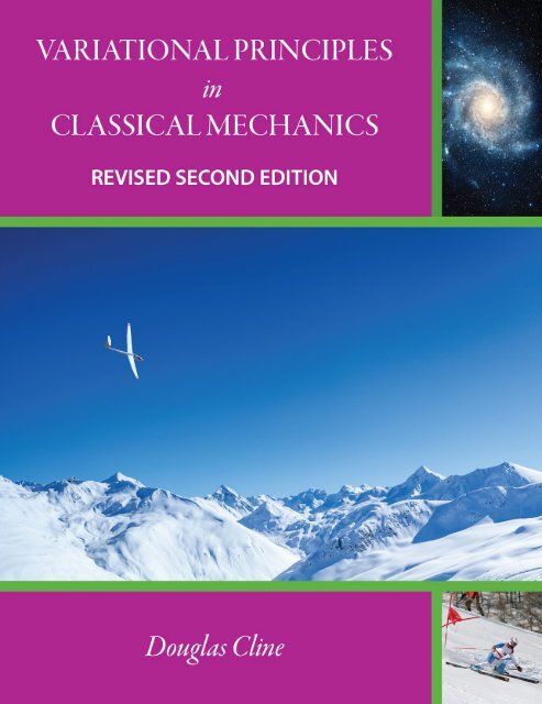
The front cover picture of this book shows a sailplane soar<strong>in</strong>g high above the Italian Alps. This picture<br />
epitomizes the unlimited horizon of opportunities provided when the full dynamic range of variational pr<strong>in</strong>ciples<br />
are applied to classical mechanics. The adjacent pictures of the galaxy, and the skier, represent the wide<br />
dynamic range of applicable topics that span from the orig<strong>in</strong> of the universe, to everyday life. These cover<br />
pictures reflect the beauty and unity of the foundation provided by variational pr<strong>in</strong>ciples to the development<br />
of classical mechanics.<br />
Information regard<strong>in</strong>g the associated P235 undergraduate course at the University of Rochester is available<br />
on the web site at http://www.pas.rochester.edu/~cl<strong>in</strong>e/P235/<strong>in</strong>dex.shtml. Information about the<br />
author is available at the Cl<strong>in</strong>e home web site: http://www.pas.rochester.edu/~cl<strong>in</strong>e/<strong>in</strong>dex.html.<br />
The author thanks Meghan Sarkis who prepared many of the illustrations, Joe Easterly who designed<br />
the book cover plus the webpage, and Moriana Garcia who organized the open-access publication. Andrew<br />
Sifa<strong>in</strong> developed the diagnostic problems <strong>in</strong>cluded <strong>in</strong> the book. The author appreciates the permission,<br />
granted by Professor Struckmeier, to quote his published article on the extended Hamilton-Lagrangian<br />
formalism. The author acknowledges the feedback and suggestions made by many students who have taken<br />
this course, as well as helpful suggestions by his colleagues; Andrew Abrams, Adam Hayes, Connie Jones,<br />
Andrew Melchionna, David Munson, Alice Quillen, Richard Sarkis, James Schneeloch, Steven Torrisi, Dan<br />
Watson, and Frank Wolfs. These lecture notes were typed <strong>in</strong> LATEX us<strong>in</strong>g Scientific WorkPlace (MacKichan<br />
Software, Inc.), while Adobe Illustrator, Photoshop, Orig<strong>in</strong>, Mathematica, and MUPAD, were used to prepare<br />
the illustrations.<br />
Douglas Cl<strong>in</strong>e,<br />
University of Rochester, <strong>2019</strong>
Prologue<br />
Two dramatically different philosophical approaches to science were developed <strong>in</strong> the field of classical mechanics<br />
dur<strong>in</strong>g the 17 - 18 centuries. This time period co<strong>in</strong>cided with the Age of Enlightenment <strong>in</strong> Europe<br />
dur<strong>in</strong>g which remarkable <strong>in</strong>tellectual and philosophical developments occurred. This was a time when both<br />
philosophical and causal arguments were equally acceptable <strong>in</strong> science, <strong>in</strong> contrast with current convention<br />
where there appears to be tacit agreement to discourage use of philosophical arguments <strong>in</strong> science.<br />
Snell’s Law: The genesis of two contrast<strong>in</strong>g philosophical approaches<br />
to science relates back to early studies of the reflection<br />
and refraction of light. The velocity of light <strong>in</strong> a medium of refractive<br />
<strong>in</strong>dex equals = <br />
. Thus a light beam <strong>in</strong>cident at an<br />
angle 1 to the normal of a plane <strong>in</strong>terface between medium 1<br />
and medium 2 isrefractedatanangle 2 <strong>in</strong> medium 2 where the<br />
angles are related by Snell’s Law.<br />
s<strong>in</strong> 1<br />
= 1<br />
= 2<br />
(Snell’s Law)<br />
s<strong>in</strong> 2 2 1<br />
Ibn Sahl of Bagdad (984) first described the refraction of light,<br />
while Snell (1621) derived his law mathematically. Both of these<br />
scientists used the “vectorial approach” where the light velocity <br />
is considered to be a vector po<strong>in</strong>t<strong>in</strong>g <strong>in</strong> the direction of propagation.<br />
Fermat’s Pr<strong>in</strong>ciple: Fermat’s pr<strong>in</strong>ciple of least time (1657),<br />
which is based on the work of Hero of Alexandria (∼ 60) and Ibn<br />
al-Haytham (1021), states that “light travels between two given<br />
po<strong>in</strong>ts along the path of shortest time”. The transit time of a<br />
light beam between two locations and <strong>in</strong> a medium with<br />
position-dependent refractive <strong>in</strong>dex () is given by<br />
=<br />
Z <br />
<br />
= 1 <br />
Z <br />
<br />
()<br />
(Fermat’s Pr<strong>in</strong>ciple)<br />
Fermat’s Pr<strong>in</strong>ciple leads to the derivation of Snell’s Law.<br />
Philosophically the physics underly<strong>in</strong>g the contrast<strong>in</strong>g vectorial<br />
and Fermat’s Pr<strong>in</strong>ciple derivations of Snell’s Law are dramatically<br />
different. The vectorial approach is based on differential relations<br />
between the velocity vectors <strong>in</strong> the two media, whereas Fermat’s<br />
variational approach is based on the fact that the light preferentially<br />
selects a path for which the <strong>in</strong>tegral of the transit time<br />
Figure 1: Vectorial and variational representations<br />
of Snell’s Law for refraction of light.<br />
between the <strong>in</strong>itial location and the f<strong>in</strong>al location is m<strong>in</strong>imized.<br />
That is, the first approach is based on “vectorial mechanics” whereas Fermat’s approach is based on<br />
variational pr<strong>in</strong>ciples <strong>in</strong> that the path between the <strong>in</strong>itial and f<strong>in</strong>al locations is varied to f<strong>in</strong>d the path that<br />
m<strong>in</strong>imizes the transit time. Fermat’s enunciation of variational pr<strong>in</strong>ciples <strong>in</strong> physics played a key role <strong>in</strong> the<br />
historical development, and subsequent exploitation, of the pr<strong>in</strong>ciple of least action <strong>in</strong> analytical formulations<br />
of classical mechanics as discussed below.<br />
xix
xx<br />
PROLOGUE<br />
Newtonian mechanics: Momentum and force are vectors that underlie the Newtonian formulation of<br />
classical mechanics. Newton’s monumental treatise, entitled “Philosophiae Naturalis Pr<strong>in</strong>cipia Mathematica”,<br />
published <strong>in</strong> 1687, established his three universal laws of motion, the universal theory of gravitation,<br />
the derivation of Kepler’s three laws of planetary motion, and the development of calculus. Newton’s three<br />
universal laws of motion provide the most <strong>in</strong>tuitive approach to classical mechanics <strong>in</strong> that they are based on<br />
vector quantities like momentum, and the rate of change of momentum, which are related to force. Newton’s<br />
equation of motion<br />
F = p<br />
(Newton’s equation of motion)<br />
<br />
is a vector differential relation between the <strong>in</strong>stantaneous forces and rate of change of momentum, or equivalent<br />
<strong>in</strong>stantaneous acceleration, all of which are vector quantities. Momentum and force are easy to visualize,<br />
and both cause and effect are embedded <strong>in</strong> Newtonian mechanics. Thus, if all of the forces, <strong>in</strong>clud<strong>in</strong>g the<br />
constra<strong>in</strong>t forces, act<strong>in</strong>g on the system are known, then the motion is solvable for two body systems. The<br />
mathematics for handl<strong>in</strong>g Newton’s “vectorial mechanics” approach to classical mechanics is well established.<br />
Analytical mechanics: <strong>Variational</strong> pr<strong>in</strong>ciples apply to many aspects of our daily life. Typical examples<br />
<strong>in</strong>clude; select<strong>in</strong>g the optimum compromise <strong>in</strong> quality and cost when shopp<strong>in</strong>g, select<strong>in</strong>g the fastest route<br />
to travel from home to work, or select<strong>in</strong>g the optimum compromise to satisfy the disparate desires of the<br />
<strong>in</strong>dividuals compris<strong>in</strong>g a family. <strong>Variational</strong> pr<strong>in</strong>ciples underlie the analytical formulation of mechanics. It<br />
is astonish<strong>in</strong>g that the laws of nature are consistent with variational pr<strong>in</strong>ciples <strong>in</strong>volv<strong>in</strong>g the pr<strong>in</strong>ciple of<br />
least action. M<strong>in</strong>imiz<strong>in</strong>g the action <strong>in</strong>tegral led to the development of the mathematical field of variational<br />
calculus, plus the analytical variational approaches to classical mechanics, by Euler, Lagrange, Hamilton,<br />
and Jacobi.<br />
Leibniz, who was a contemporary of Newton, <strong>in</strong>troduced methods based on a quantity called “vis viva”,<br />
which is Lat<strong>in</strong> for “liv<strong>in</strong>g force” and equals twice the k<strong>in</strong>etic energy. Leibniz believed <strong>in</strong> the philosophy<br />
that God created a perfect world where nature would be thrifty <strong>in</strong> all its manifestations. In 1707, Leibniz<br />
proposed that the optimum path is based on m<strong>in</strong>imiz<strong>in</strong>g the time <strong>in</strong>tegral of the vis viva, which is equivalent<br />
to the action <strong>in</strong>tegral of Lagrangian/Hamiltonian mechanics. In 1744 Euler derived the Leibniz result<br />
us<strong>in</strong>g variational concepts while Maupertuis restated the Leibniz result based on teleological arguments.<br />
The development of Lagrangian mechanics culm<strong>in</strong>ated <strong>in</strong> the 1788 publication of Lagrange’s monumental<br />
treatise entitled “Mécanique Analytique”. Lagrange used d’Alembert’s Pr<strong>in</strong>ciple to derive Lagrangian mechanics<br />
provid<strong>in</strong>g a powerful analytical approach to determ<strong>in</strong>e the magnitude and direction of the optimum<br />
trajectories, plus the associated forces.<br />
The culm<strong>in</strong>ation of the development of analytical mechanics occurred <strong>in</strong> 1834 when Hamilton proposed<br />
his Pr<strong>in</strong>ciple of Least Action, as well as develop<strong>in</strong>g Hamiltonian mechanics which is the premier variational<br />
approach <strong>in</strong> science. Hamilton’s concept of least action is def<strong>in</strong>ed to be the time <strong>in</strong>tegral of the Lagrangian.<br />
Hamilton’s Action Pr<strong>in</strong>ciple (1834) m<strong>in</strong>imizes the action <strong>in</strong>tegral def<strong>in</strong>ed by<br />
=<br />
Z <br />
<br />
(q ˙q)<br />
(Hamilton’s Pr<strong>in</strong>ciple)<br />
In the simplest form, the Lagrangian (q ˙q) equals the difference between the k<strong>in</strong>etic energy and the<br />
potential energy . Hamilton’s Least Action Pr<strong>in</strong>ciple underlies Lagrangian mechanics. This Lagrangian is<br />
a function of generalized coord<strong>in</strong>ates plus their correspond<strong>in</strong>g velocities ˙ . Hamilton also developed<br />
the premier variational approach, called Hamiltonian mechanics, that is based on the Hamiltonian (q p)<br />
which is a function of the fundamental position plus the conjugate momentum variables. In 1843<br />
Jacobi provided the mathematical framework required to fully exploit the power of Hamiltonian mechanics.<br />
Note that the Lagrangian, Hamiltonian, and the action <strong>in</strong>tegral, all are scalar quantities which simplifies<br />
derivation of the equations of motion compared with the vector calculus used by Newtonian mechanics.<br />
Figure 2 presents a philosophical roadmap illustrat<strong>in</strong>g the hierarchy of philosophical approaches based on<br />
Hamilton’s Action Pr<strong>in</strong>ciple, that are available for deriv<strong>in</strong>g the equations of motion of a system. The primary<br />
Stage1 uses Hamilton’s Action functional, = R <br />
<br />
(q ˙q) to derive the Lagrangian, and Hamiltonian<br />
functionals which provide the most fundamental and sophisticated level of understand<strong>in</strong>g. Stage1 <strong>in</strong>volves<br />
specify<strong>in</strong>g all the active degrees of freedom, as well as the <strong>in</strong>teractions <strong>in</strong>volved. Stage2 uses the Lagrangian<br />
or Hamiltonian functionals, derived at Stage1, <strong>in</strong> order to derive the equations of motion for the system of
xxi<br />
Hamilton’s action pr<strong>in</strong>ciple<br />
Stage 1<br />
Stage 2<br />
Hamiltonian<br />
Lagrangian<br />
d’ Alembert’s Pr<strong>in</strong>ciple<br />
Equations of motion<br />
Newtonian mechanics<br />
Stage 3<br />
Solution for motion<br />
Initial conditions<br />
Figure 2: Philosophical road map of the hierarchy of stages <strong>in</strong>volved <strong>in</strong> analytical mechanics. Hamilton’s<br />
Action Pr<strong>in</strong>ciple is the foundation of analytical mechanics. Stage 1 uses Hamilton’s Pr<strong>in</strong>ciple to derive the<br />
Lagranian and Hamiltonian. Stage 2 uses either the Lagrangian or Hamiltonian to derive the equations<br />
of motion for the system. Stage 3 uses these equations of motion to solve for the actual motion us<strong>in</strong>g<br />
the assumed <strong>in</strong>itial conditions. The Lagrangian approach can be derived directly based on d’Alembert’s<br />
Pr<strong>in</strong>ciple. Newtonian mechanics can be derived directly based on Newton’s Laws of Motion. The advantages<br />
and power of Hamilton’s Action Pr<strong>in</strong>ciple are unavailable if the Laws of Motion are derived us<strong>in</strong>g either<br />
d’Alembert’s Pr<strong>in</strong>ciple or Newton’s Laws of Motion.<br />
<strong>in</strong>terest. Stage3 then uses these derived equations of motion to solve for the motion of the system subject to<br />
a given set of <strong>in</strong>itial boundary conditions. Note that Lagrange first derived Lagrangian mechanics based on<br />
d’ Alembert’s Pr<strong>in</strong>ciple, while Newton’s Laws of Motion specify the equations of motion used <strong>in</strong> Newtonian<br />
mechanics.<br />
The analytical approach to classical mechanics appeared contradictory to Newton’s <strong>in</strong>tuitive vectorial<br />
treatment of force and momentum. There is a dramatic difference <strong>in</strong> philosophy between the vectordifferential<br />
equations of motion derived by Newtonian mechanics, which relate the <strong>in</strong>stantaneous force to<br />
the correspond<strong>in</strong>g <strong>in</strong>stantaneous acceleration, and analytical mechanics, where m<strong>in</strong>imiz<strong>in</strong>g the scalar action<br />
<strong>in</strong>tegral <strong>in</strong>volves <strong>in</strong>tegrals over space and time between specified <strong>in</strong>itial and f<strong>in</strong>al states. Analytical mechanics<br />
uses variational pr<strong>in</strong>ciples to determ<strong>in</strong>e the optimum trajectory, from a cont<strong>in</strong>uum of tentative possibilities,<br />
by requir<strong>in</strong>g that the optimum trajectory m<strong>in</strong>imizes the action <strong>in</strong>tegral between specified <strong>in</strong>itial and f<strong>in</strong>al<br />
conditions.<br />
Initially there was considerable prejudice and philosophical opposition to use of the variational pr<strong>in</strong>ciples<br />
approach which is based on the assumption that nature follows the pr<strong>in</strong>ciples of economy. The variational<br />
approach is not <strong>in</strong>tuitive, and thus it was considered to be speculative and “metaphysical”, but it was<br />
tolerated as an efficient tool for exploit<strong>in</strong>g classical mechanics. This opposition to the variational pr<strong>in</strong>ciples<br />
underly<strong>in</strong>g analytical mechanics, delayed full appreciation of the variational approach until the start of the<br />
20 century. As a consequence, the <strong>in</strong>tuitive Newtonian formulation reigned supreme <strong>in</strong> classical mechanics<br />
for over two centuries, even though the remarkable problem-solv<strong>in</strong>g capabilities of analytical mechanics were<br />
recognized and exploited follow<strong>in</strong>g the development of analytical mechanics by Lagrange.<br />
The full significance and superiority of the analytical variational formulations of classical mechanics<br />
became well recognised and accepted follow<strong>in</strong>g the development of the Special Theory of Relativity <strong>in</strong> 1905.<br />
The Theory of Relativity requires that the laws of nature be <strong>in</strong>variant to the reference frame. This is not<br />
satisfied by the Newtonian formulation of mechanics which assumes one absolute frame of reference and a<br />
separation of space and time. In contrast, the Lagrangian and Hamiltonian formulations of the pr<strong>in</strong>ciple of<br />
least action rema<strong>in</strong> valid <strong>in</strong> the Theory of Relativity, if the Lagrangian is written <strong>in</strong> a relativistically-<strong>in</strong>variant
xxii<br />
PROLOGUE<br />
form <strong>in</strong> space-time. The complete <strong>in</strong>variance of the variational approach to coord<strong>in</strong>ate frames is precisely<br />
the formalism necessary for handl<strong>in</strong>g relativistic mechanics.<br />
Hamiltonian mechanics, which is expressed <strong>in</strong> terms of the conjugate variables (q p), relates classical<br />
mechanics directly to the underly<strong>in</strong>g physics of quantum mechanics and quantum field theory. As a consequence,<br />
the philosophical opposition to exploit<strong>in</strong>g variational pr<strong>in</strong>ciples no longer exists, and Hamiltonian<br />
mechanics has become the preem<strong>in</strong>ent formulation of modern physics. The reader is free to draw their own<br />
conclusions regard<strong>in</strong>g the philosophical question “is the pr<strong>in</strong>ciple of economy a fundamental law of classical<br />
mechanics, or is it a fortuitous consequence of the fundamental laws of nature?”<br />
From the late seventeenth century, until the dawn of modern physics at the start of the twentieth century,<br />
classical mechanics rema<strong>in</strong>ed a primary driv<strong>in</strong>g force <strong>in</strong> the development of physics. <strong>Classical</strong> mechanics<br />
embraces an unusually broad range of topics spann<strong>in</strong>g motion of macroscopic astronomical bodies to microscopic<br />
particles <strong>in</strong> nuclear and particle physics, at velocities rang<strong>in</strong>g from zero to near the velocity of<br />
light, from one-body to statistical many-body systems, as well as hav<strong>in</strong>g extensions to quantum mechanics.<br />
Introduction of the Special Theory of Relativity <strong>in</strong> 1905, and the General Theory of Relativity <strong>in</strong> 1916,<br />
necessitated modifications to classical mechanics for relativistic velocities, and can be considered to be an<br />
extended theory of classical mechanics. S<strong>in</strong>ce the 1920 0 s, quantal physics has superseded classical mechanics<br />
<strong>in</strong> the microscopic doma<strong>in</strong>. Although quantum physics has played the lead<strong>in</strong>g role <strong>in</strong> the development of<br />
physics dur<strong>in</strong>g much of the past century, classical mechanics still is a vibrant field of physics that recently<br />
has led to excit<strong>in</strong>g developments associated with non-l<strong>in</strong>ear systems and chaos theory. This has spawned<br />
new branches of physics and mathematics as well as chang<strong>in</strong>g our notion of causality.<br />
Goals: The primary goal of this book is to <strong>in</strong>troduce the reader to the powerful variational-pr<strong>in</strong>ciples<br />
approaches that play such a pivotal role <strong>in</strong> classical mechanics and many other branches of modern science<br />
and eng<strong>in</strong>eer<strong>in</strong>g. This book emphasizes the <strong>in</strong>tellectual beauty of these remarkable developments, as well as<br />
stress<strong>in</strong>g the philosophical implications that have had a tremendous impact on modern science. A secondary<br />
goal is to apply variational pr<strong>in</strong>ciples to solve advanced applications <strong>in</strong> classical mechanics <strong>in</strong> order to<br />
<strong>in</strong>troduce many sophisticated and powerful mathematical techniques that underlie much of modern physics.<br />
This book starts with a review of Newtonian mechanics plus the solutions of the correspond<strong>in</strong>g equations<br />
of motion. This is followed by an <strong>in</strong>troduction to Lagrangian mechanics, based on d’Alembert’s Pr<strong>in</strong>ciple,<br />
<strong>in</strong> order to develop familiarity <strong>in</strong> apply<strong>in</strong>g variational pr<strong>in</strong>ciples to classical mechanics. This leads to <strong>in</strong>troduction<br />
of the more fundamental Hamilton’s Action Pr<strong>in</strong>ciple, plus Hamiltonian mechanics, to illustrate the<br />
power provided by exploit<strong>in</strong>g the full hierarchy of stages available for apply<strong>in</strong>g variational pr<strong>in</strong>ciples to classical<br />
mechanics. F<strong>in</strong>ally the book illustrates how variational pr<strong>in</strong>ciples <strong>in</strong> classical mechanics were exploited<br />
dur<strong>in</strong>g the development of both relativisitic mechanics and quantum physics. The connections and applications<br />
of classical mechanics to modern physics, are emphasized throughout the book <strong>in</strong> an effort to span the<br />
chasm that divides the Newtonian vector-differential formulation, and the <strong>in</strong>tegral variational formulation, of<br />
classical mechanics. This chasm is especially applicable to quantum mechanics which is based completely on<br />
variational pr<strong>in</strong>ciples. Note that variational pr<strong>in</strong>ciples, developed <strong>in</strong> the field of classical mechanics, now are<br />
used <strong>in</strong> a diverse and wide range of fields outside of physics, <strong>in</strong>clud<strong>in</strong>g economics, meteorology, eng<strong>in</strong>eer<strong>in</strong>g,<br />
and comput<strong>in</strong>g.<br />
This study of classical mechanics <strong>in</strong>volves climb<strong>in</strong>g a vast mounta<strong>in</strong> of knowledge, and the pathway to the<br />
top leads to elegant and beautiful theories that underlie much of modern physics. This book exploits variational<br />
pr<strong>in</strong>ciples applied to four major topics <strong>in</strong> classical mechanics to illustrate the power and importance of<br />
variational pr<strong>in</strong>ciples <strong>in</strong> physics. Be<strong>in</strong>g so close to the summit provides the opportunity to take a few extra<br />
steps beyond the normal <strong>in</strong>troductory classical mechanics syllabus to glimpse the excit<strong>in</strong>g physics found at<br />
the summit. This new physics <strong>in</strong>cludes topics such as quantum, relativistic, and statistical mechanics.
Chapter 1<br />
A brief history of classical mechanics<br />
1.1 Introduction<br />
This chapter reviews the historical evolution of classical mechanics s<strong>in</strong>ce considerable <strong>in</strong>sight can be ga<strong>in</strong>ed<br />
from study of the history of science. There are two dramatically different approaches used <strong>in</strong> classical<br />
mechanics. The first is the vectorial approach of Newton which is based on vector quantities like momentum,<br />
force, and acceleration. The second is the analytical approach of Lagrange, Euler, Hamilton, and Jacobi,<br />
that is based on the concept of least action and variational calculus. The more <strong>in</strong>tuitive Newtonian picture<br />
reigned supreme <strong>in</strong> classical mechanics until the start of the twentieth century. <strong>Variational</strong> pr<strong>in</strong>ciples, which<br />
were developed dur<strong>in</strong>g the n<strong>in</strong>eteenth century, never aroused much enthusiasm <strong>in</strong> scientific circles due to<br />
philosophical objections to the underly<strong>in</strong>g concepts;thisapproachwasmerelytoleratedasanefficient tool<br />
for exploit<strong>in</strong>g classical mechanics. A dramatic advance <strong>in</strong> the philosophy of science occurred at the start of<br />
the 20 century lead<strong>in</strong>g to widespread acceptance of the superiority of us<strong>in</strong>g variational pr<strong>in</strong>ciples.<br />
1.2 Greek antiquity<br />
The great philosophers <strong>in</strong> ancient Greece played a key role by us<strong>in</strong>g the astronomical work of the Babylonians<br />
to develop scientific theories of mechanics. Thales of Miletus (624 - 547BC), thefirst of the seven<br />
great greek philosophers, developed geometry, and is hailed as the first true mathematician. Pythagorus<br />
(570 - 495BC) developed mathematics, and postulated that the earth is spherical. Democritus (460 -<br />
370BC) has been called the father of modern science, while Socrates (469 - 399BC) is renowned for his<br />
contributions to ethics. Plato (427-347 B.C.) who was a mathematician and student of Socrates, wrote<br />
important philosophical dialogues. He founded the Academy <strong>in</strong> Athens which was the first <strong>in</strong>stitution of<br />
higher learn<strong>in</strong>g <strong>in</strong> the Western world that helped lay the foundations of Western philosophy and science.<br />
Aristotle (384-322 B.C.) is an important founder of Western philosophy encompass<strong>in</strong>g ethics, logic,<br />
science, and politics. His views on the physical sciences profoundly <strong>in</strong>fluenced medieval scholarship that<br />
extended well <strong>in</strong>to the Renaissance. He presented the first implied formulation of the pr<strong>in</strong>ciple of virtual<br />
work <strong>in</strong> statics, and his statement that “what is lost <strong>in</strong> velocity is ga<strong>in</strong>ed <strong>in</strong> force” is a veiled reference to<br />
k<strong>in</strong>etic and potential energy. He adopted an Earth centered model of the universe. Aristarchus (310 - 240<br />
B.C.) argued that the Earth orbited the Sun and used measurements to imply the relative distances of the<br />
Moon and the Sun. The greek philosophers were relatively advanced <strong>in</strong> logic and mathematics and developed<br />
concepts that enabled them to calculate areas and perimeters. Unfortunately their philosophical approach<br />
neglected collect<strong>in</strong>g quantitative and systematic data that is an essential <strong>in</strong>gredient to the advancement of<br />
science.<br />
Archimedes (287-212 B.C.) represented the culm<strong>in</strong>ation of science <strong>in</strong> ancient Greece. As an eng<strong>in</strong>eer<br />
he designed mach<strong>in</strong>es of war, while as a scientist he made significant contributions to hydrostatics and<br />
the pr<strong>in</strong>ciple of the lever. As a mathematician, he applied <strong>in</strong>f<strong>in</strong>itessimals <strong>in</strong> a way that is rem<strong>in</strong>iscent of<br />
modern <strong>in</strong>tegral calculus, which he used to derive a value for Unfortunately much of the work of the<br />
brilliant Archimedes subsequently fell <strong>in</strong>to oblivion. Hero of Alexandria (10 - 70 A.D.) described the<br />
pr<strong>in</strong>ciple of reflection that light takes the shortest path. This is an early illustration of variational pr<strong>in</strong>ciple<br />
1
2 CHAPTER 1. A BRIEF HISTORY OF CLASSICAL MECHANICS<br />
of least time. Ptolemy (83 - 161 A.D.) wrote several scientific treatises that greatly <strong>in</strong>fluenced subsequent<br />
philosophers. Unfortunately he adopted the <strong>in</strong>correct geocentric solar system <strong>in</strong> contrast to the heliocentric<br />
model of Aristarchus and others.<br />
1.3 Middle Ages<br />
Thedecl<strong>in</strong>eandfalloftheRomanEmpire<strong>in</strong>∼410 A.D. marks the end of <strong>Classical</strong> Antiquity, and the<br />
beg<strong>in</strong>n<strong>in</strong>g of the Dark Ages <strong>in</strong> Western Europe (Christendom), while the Muslim scholars <strong>in</strong> Eastern Europe<br />
cont<strong>in</strong>ued to make progress <strong>in</strong> astronomy and mathematics. For example, <strong>in</strong> Egypt, Alhazen (965 - 1040<br />
A.D.) expanded the pr<strong>in</strong>ciple of least time to reflection and refraction. The Dark Ages <strong>in</strong>volved a long<br />
scientific decl<strong>in</strong>e <strong>in</strong> Western Europe that languished for about 900 years. Science was dom<strong>in</strong>ated by religious<br />
dogma, all western scholars were monks, and the important scientific achievements of Greek antiquity were<br />
forgotten. The works of Aristotle were re<strong>in</strong>troduced to Western Europe by Arabs <strong>in</strong> the early 13 century<br />
lead<strong>in</strong>g to the concepts of forces <strong>in</strong> static systems which were developed dur<strong>in</strong>g the fourteenth century.<br />
This <strong>in</strong>cluded concepts of the work done by a force, and the virtual work <strong>in</strong>volved <strong>in</strong> virtual displacements.<br />
Leonardo da V<strong>in</strong>ci (1452-1519) was a leader <strong>in</strong> mechanics at that time. He made sem<strong>in</strong>al contributions<br />
to science, <strong>in</strong> addition to his well known contributions to architecture, eng<strong>in</strong>eer<strong>in</strong>g, sculpture, and art.<br />
Nicolaus Copernicus (1473-1543) rejected the geocentric theory of Ptolomy and formulated a scientificallybased<br />
heliocentric cosmology that displaced the Earth from the center of the universe. The Ptolomic view<br />
was that heaven represented the perfect unchang<strong>in</strong>g div<strong>in</strong>e while the earth represented change plus chaos,<br />
and the celestial bodies moved relative to the fixed heavens. The book, De revolutionibus orbium coelestium<br />
(On the Revolutions of the Celestial Spheres), published by Copernicus <strong>in</strong> 1543, is regarded as the start<strong>in</strong>g<br />
po<strong>in</strong>t of modern astronomy and the def<strong>in</strong><strong>in</strong>g epiphany that began the Scientific Revolution. ThebookDe<br />
Magnete written <strong>in</strong> 1600 by the English physician William Gilbert (1540-1603) presented the results of<br />
well-planned studies of magnetism and strongly <strong>in</strong>fluenced the <strong>in</strong>tellectual-scientific evolution at that time.<br />
Johannes Kepler (1571-1630), a German mathematician, astronomer and astrologer, was a key<br />
figure <strong>in</strong> the 17th century Scientific Revolution. He is best known for recogniz<strong>in</strong>g the connection between the<br />
motions <strong>in</strong> the sky and physics. His laws of planetary motion were developed by later astronomers based on<br />
his written work Astronomia nova, Harmonices Mundi, andEpitome of Copernican Astrononomy. Kepler<br />
was an assistant to Tycho Brahe (1546-1601) who for many years recorded accurate astronomical data<br />
that played a key role <strong>in</strong> the development of Kepler’s theory of planetary motion. Kepler’s work provided<br />
the foundation for Isaac Newton’s theory of universal gravitation. Unfortunately Kepler did not recognize<br />
the true nature of the gravitational force.<br />
Galileo Galilei (1564-1642) built on the Aristotle pr<strong>in</strong>ciple by recogniz<strong>in</strong>g the law of <strong>in</strong>ertia, the<br />
persistence of motion if no forces act, and the proportionality between force and acceleration. This amounts<br />
to recognition of work as the product of force times displacement <strong>in</strong> the direction of the force. He applied<br />
virtual work to the equilibrium of a body on an <strong>in</strong>cl<strong>in</strong>ed plane. He also showed that the same pr<strong>in</strong>ciple<br />
applies to hydrostatic pressure that had been established by Archimedes, but he did not apply his concepts<br />
<strong>in</strong> classical mechanics to the considerable knowledge base on planetary motion. Galileo is famous for the<br />
apocryphal story that he dropped two cannon balls of differentmassesfromtheTowerofPisatodemonstrate<br />
that their speed of descent was <strong>in</strong>dependent of their mass.<br />
1.4 Age of Enlightenment<br />
The Age of Enlightenment is a term used to describe a phase <strong>in</strong> Western philosophy and cultural life <strong>in</strong><br />
which reason was advocated as the primary source and legitimacy for authority. It developed simultaneously<br />
<strong>in</strong> Germany, France, Brita<strong>in</strong>, the Netherlands, and Italy around the 1650’s and lasted until the French<br />
Revolution <strong>in</strong> 1789. The <strong>in</strong>tellectual and philosophical developments led to moral, social, and political<br />
reforms. The pr<strong>in</strong>ciples of <strong>in</strong>dividual rights, reason, common sense, and deism were a revolutionary departure<br />
from the exist<strong>in</strong>g theocracy, autocracy, oligarchy, aristocracy, and the div<strong>in</strong>e right of k<strong>in</strong>gs. It led to political<br />
revolutions <strong>in</strong> France and the United States. It marks a dramatic departure from the Early Modern period<br />
which was noted for religious authority, absolute state power, guild-based economic systems, and censorship<br />
of ideas. It opened a new era of rational discourse, liberalism, freedom of expression, and scientific method.<br />
This new environment led to tremendous advances <strong>in</strong> both science and mathematics <strong>in</strong> addition to music,
1.4. AGE OF ENLIGHTENMENT 3<br />
literature, philosophy, and art. Scientific development dur<strong>in</strong>g the 17 century <strong>in</strong>cluded the pivotal advances<br />
made by Newton and Leibniz at the beg<strong>in</strong>n<strong>in</strong>g of the revolutionary Age of Enlightenment, culm<strong>in</strong>at<strong>in</strong>g <strong>in</strong> the<br />
development of variational calculus and analytical mechanics by Euler and Lagrange. The scientific advances<br />
of this age <strong>in</strong>clude publication of two monumental books Philosophiae Naturalis Pr<strong>in</strong>cipia Mathematica by<br />
Newton <strong>in</strong> 1687 and Mécanique analytique by Lagrange <strong>in</strong> 1788. These are the def<strong>in</strong>itive two books upon<br />
which classical mechanics is built.<br />
René Descartes (1596-1650) attempted to formulate the laws of motion <strong>in</strong> 1644. He talked about<br />
conservation of motion (momentum) <strong>in</strong> a straight l<strong>in</strong>e but did not recognize the vector character of momentum.<br />
Pierre de Fermat (1601-1665) and René Descartes were two lead<strong>in</strong>g mathematicians <strong>in</strong> the first<br />
half of the 17 century. Independently they discovered the pr<strong>in</strong>ciples of analytic geometry and developed<br />
some <strong>in</strong>itial concepts of calculus. Fermat and Blaise Pascal (1623-1662) were the founders of the theory<br />
of probability.<br />
Isaac Newton (1642-1727) made pioneer<strong>in</strong>g contributions to physics and mathematics as well as<br />
be<strong>in</strong>g a theologian. At 18 he was admitted to Tr<strong>in</strong>ity College Cambridge where he read the writ<strong>in</strong>gs of<br />
modern philosophers like Descartes, and astronomers like Copernicus, Galileo, and Kepler. By 1665 he had<br />
discovered the generalized b<strong>in</strong>omial theorem, and began develop<strong>in</strong>g <strong>in</strong>f<strong>in</strong>itessimal calculus. Due to a plague,<br />
the university closed for two years <strong>in</strong> 1665 dur<strong>in</strong>g which Newton worked at home develop<strong>in</strong>g the theory<br />
of calculus that built upon the earlier work of Barrow and Descartes. He was elected Lucasian Professor<br />
of Mathematics <strong>in</strong> 1669 at the age of 26. From 1670 Newton focussed on optics lead<strong>in</strong>g to his Hypothesis<br />
of Light published <strong>in</strong> 1675 and his book Opticks <strong>in</strong> 1704. Newton described light as be<strong>in</strong>g made up of a<br />
flow of extremely subtle corpuscles that also had associated wavelike properties to expla<strong>in</strong> diffraction and<br />
optical <strong>in</strong>terference that he studied. Newton returned to mechanics <strong>in</strong> 1677 by study<strong>in</strong>g planetary motion<br />
and gravitation that applied the calculus he had developed. In 1687 he published his monumental treatise<br />
entitled Philosophiae Naturalis Pr<strong>in</strong>cipia Mathematica which established his three universal laws of motion,<br />
the universal theory of gravitation, derivation of Kepler’s three laws of planetary motion, and was his first<br />
publication of the development of calculus which he called “the science of fluxions”. Newton’s laws of motion<br />
are based on the concepts of force and momentum, that is, force equals the rate of change of momentum.<br />
Newton’s postulate of an <strong>in</strong>visible force able to act over vast distances led him to be criticized for <strong>in</strong>troduc<strong>in</strong>g<br />
“occult agencies” <strong>in</strong>to science. In a remarkable achievement, Newton completely solved the laws of mechanics.<br />
His theory of classical mechanics and of gravitation reigned supreme until the development of the Theory<br />
of Relativity <strong>in</strong> 1905. The followers of Newton envisioned the Newtonian laws to be absolute and universal.<br />
This dogmatic reverence of Newtonian mechanics prevented physicists from an unprejudiced appreciation of<br />
the analytic variational approach to mechanics developed dur<strong>in</strong>g the 17 through 19 centuries. Newton<br />
was the first scientist to be knighted and was appo<strong>in</strong>ted president of the Royal Society.<br />
Gottfried Leibniz (1646-1716) was a brilliant German philosopher, a contemporary of Newton, who<br />
worked on both calculus and mechanics. Leibniz started development of calculus <strong>in</strong> 1675, ten years after<br />
Newton, but Leibniz published his work <strong>in</strong> 1684, which was three years before Newton’s Pr<strong>in</strong>cipia. Leibniz<br />
made significant contributions to <strong>in</strong>tegral calculus and developed the notation currently used <strong>in</strong> calculus.<br />
He <strong>in</strong>troduced the name calculus based on the Lat<strong>in</strong> word for the small stone used for count<strong>in</strong>g. Newton<br />
and Leibniz were <strong>in</strong>volved <strong>in</strong> a protracted argument over who orig<strong>in</strong>ated calculus. It appears that Leibniz<br />
saw drafts of Newton’s work on calculus dur<strong>in</strong>g a visit to England. Throughout their argument Newton<br />
was the ghost writer of most of the articles <strong>in</strong> support of himself and he had them published under nonde-plume<br />
of his friends. Leibniz made the tactical error of appeal<strong>in</strong>g to the Royal Society to <strong>in</strong>tercede on<br />
his behalf. Newton, as president of the Royal Society, appo<strong>in</strong>ted his friends to an “impartial” committee to<br />
<strong>in</strong>vestigate this issue, then he wrote the committee’s report that accused Leibniz of plagiarism of Newton’s<br />
work on calculus, after which he had it published by the Royal Society. Still unsatisfied he then wrote an<br />
anonymous review of the report <strong>in</strong> the Royal Society’s own periodical. This bitter dispute lasted until the<br />
death of Leibniz. When Leibniz died his work was largely discredited. The fact that he falsely claimed to be<br />
a nobleman and added the prefix “von” to his name, coupled with Newton’s vitriolic attacks, did not help<br />
his credibility. Newton is reported to have declared that he took great satisfaction <strong>in</strong> “break<strong>in</strong>g Leibniz’s<br />
heart.” Studies dur<strong>in</strong>g the 20 century have largely revived the reputation of Leibniz and he is recognized<br />
to have made major contributions to the development of calculus.
4 CHAPTER 1. A BRIEF HISTORY OF CLASSICAL MECHANICS<br />
Figure 1.1: Chronological roadmap of the parallel development of the Newtonian and <strong>Variational</strong>-pr<strong>in</strong>ciples<br />
approaches to classical mechanics.
1.5. VARIATIONAL METHODS IN PHYSICS 5<br />
1.5 <strong>Variational</strong> methods <strong>in</strong> physics<br />
Pierre de Fermat (1601-1665) revived the pr<strong>in</strong>ciple of least time, which states that light travels between<br />
two given po<strong>in</strong>ts along the path of shortest time and was used to derive Snell’s law <strong>in</strong> 1657. This enunciation<br />
of variational pr<strong>in</strong>ciples <strong>in</strong> physics played a key role <strong>in</strong> the historical development of the variational pr<strong>in</strong>ciple<br />
of least action that underlies the analytical formulations of classical mechanics.<br />
Gottfried Leibniz (1646-1716) made significant contributions to the development of variational pr<strong>in</strong>ciples<br />
<strong>in</strong> classical mechanics. In contrast to Newton’s laws of motion, which are based on the concept of<br />
momentum, Leibniz devised a new theory of dynamics based on k<strong>in</strong>etic and potential energy that anticipates<br />
the analytical variational approach of Lagrange and Hamilton. Leibniz argued for a quantity called the “vis<br />
viva”, which is Lat<strong>in</strong> for liv<strong>in</strong>g force, that equals twice the k<strong>in</strong>etic energy. Leibniz argued that the change<br />
<strong>in</strong> k<strong>in</strong>etic energy is equal to the work done. In 1687 Leibniz proposed that the optimum path is based on<br />
m<strong>in</strong>imiz<strong>in</strong>g the time <strong>in</strong>tegral of the vis viva, which is equivalent to the action <strong>in</strong>tegral. Leibniz used both<br />
philosophical and causal arguments <strong>in</strong> his work which were acceptable dur<strong>in</strong>g the Age of Enlightenment. Unfortunately<br />
for Leibniz, his analytical approach based on energies, which are scalars, appeared contradictory<br />
to Newton’s <strong>in</strong>tuitive vectorial treatment of force and momentum. There was considerable prejudice and<br />
philosophical opposition to the variational approach which assumes that nature is thrifty <strong>in</strong> all of its actions.<br />
The variational approach was considered to be speculative and “metaphysical” <strong>in</strong> contrast to the causal<br />
arguments support<strong>in</strong>g Newtonian mechanics. This opposition delayed full appreciation of the variational<br />
approach until the start of the 20 century.<br />
Johann Bernoulli (1667-1748) was a Swiss mathematician who was a student of Leibniz’s calculus, and<br />
sided with Leibniz <strong>in</strong> the Newton-Leibniz dispute over the credit for develop<strong>in</strong>g calculus. Also Bernoulli sided<br />
with the Descartes’ vortex theory of gravitation which delayed acceptance of Newton’s theory of gravitation<br />
<strong>in</strong> Europe. Bernoulli pioneered development of the calculus of variations by solv<strong>in</strong>g the problems of the<br />
catenary, the brachistochrone, and Fermat’s pr<strong>in</strong>ciple. Johann Bernoulli’s son Daniel played a significant<br />
role <strong>in</strong> the development of the well-known Bernoulli Pr<strong>in</strong>ciple <strong>in</strong> hydrodynamics.<br />
Pierre Louis Maupertuis (1698-1759) was a student of Johann Bernoulli and conceived the universal<br />
hypothesis that <strong>in</strong> nature there is a certa<strong>in</strong> quantity called action which is m<strong>in</strong>imized. Although this bold<br />
assumption correctly anticipates the development of the variational approach to classical mechanics, he<br />
obta<strong>in</strong>ed his hypothesis by an entirely <strong>in</strong>correct method. He was a dilettante whose mathematical prowess<br />
was beh<strong>in</strong>d the high standards of that time, and he could not establish satisfactorily the quantity to be<br />
m<strong>in</strong>imized. His teleological 1 argument was <strong>in</strong>fluenced by Fermat’s pr<strong>in</strong>ciple and the corpuscle theory of light<br />
that implied a close connection between optics and mechanics.<br />
Leonhard Euler (1707-1783) was the preem<strong>in</strong>ent Swiss mathematician of the 18 century and was<br />
a student of Johann Bernoulli. Euler developed, with full mathematical rigor, the calculus of variations<br />
follow<strong>in</strong>g <strong>in</strong> the footsteps of Johann Bernoulli. Euler used variational calculus to solve m<strong>in</strong>imum/maximum<br />
isoperimetric problems that had attracted and challenged the early developers of calculus, Newton, Leibniz,<br />
and Bernoulli. Euler also was the first to solve the rigid-body rotation problem us<strong>in</strong>g the three components<br />
of the angular velocity as k<strong>in</strong>ematical variables. Euler became bl<strong>in</strong>d <strong>in</strong> both eyes by 1766 but that did not<br />
h<strong>in</strong>der his prolific output <strong>in</strong> mathematics due to his remarkable memory and mental capabilities. Euler’s<br />
contributions to mathematics are remarkable <strong>in</strong> quality and quantity; for example dur<strong>in</strong>g 1775 he published<br />
one mathematical paper per week <strong>in</strong> spite of be<strong>in</strong>g bl<strong>in</strong>d. Euler implicitly implied the pr<strong>in</strong>ciple of least<br />
action us<strong>in</strong>g vis visa which is not the exact form explicitly developed by Lagrange.<br />
Jean le Rond d’Alembert (1717-1785) was a French mathematician and physicist who had the<br />
clever idea of extend<strong>in</strong>g use of the pr<strong>in</strong>ciple of virtual work from statics to dynamics. d’Alembert’s Pr<strong>in</strong>ciple<br />
rewrites the pr<strong>in</strong>ciple of virtual work <strong>in</strong> the form<br />
X<br />
(F − ṗ )r =0<br />
=1<br />
where the <strong>in</strong>ertial reaction force ṗ is subtracted from the correspond<strong>in</strong>g force F. This extension of the<br />
pr<strong>in</strong>ciple of virtual work applies equally to both statics and dynamics lead<strong>in</strong>g to a s<strong>in</strong>gle variational pr<strong>in</strong>ciple.<br />
Joseph Louis Lagrange (1736-1813) was an Italian mathematician and a student of Leonhard Euler.<br />
In 1788 Lagrange published his monumental treatise on analytical mechanics entitled Mécanique Analytique<br />
1 Teleology is any philosophical account that holds that f<strong>in</strong>al causes exist <strong>in</strong> nature, analogous to purposes found <strong>in</strong> human<br />
actions, nature <strong>in</strong>herently tends toward def<strong>in</strong>ite ends.
6 CHAPTER 1. A BRIEF HISTORY OF CLASSICAL MECHANICS<br />
which <strong>in</strong>troduces his Lagrangian mechanics analytical technique which is based on d’Alembert’s Pr<strong>in</strong>ciple of<br />
Virtual Work. Lagrangian mechanics is a remarkably powerful technique that is equivalent to m<strong>in</strong>imiz<strong>in</strong>g<br />
the action <strong>in</strong>tegral def<strong>in</strong>ed as<br />
=<br />
Z 2<br />
1<br />
The Lagrangian frequently is def<strong>in</strong>ed to be the difference between the k<strong>in</strong>etic energy and potential<br />
energy . His theory only required the analytical form of these scalar quantities. In the preface of his<br />
book he refers modestly to his extraord<strong>in</strong>ary achievements with the statement “The reader will f<strong>in</strong>d no<br />
figures <strong>in</strong> the work. The methods which I set forth do not require either constructions or geometrical or<br />
mechanical reason<strong>in</strong>gs: but only algebraic operations, subject to a regular and uniform rule of procedure.”<br />
Lagrange also <strong>in</strong>troduced the concept of undeterm<strong>in</strong>ed multipliers to handle auxiliary conditions which<br />
plays a vital part of theoretical mechanics. William Hamilton, an outstand<strong>in</strong>g figure <strong>in</strong> the analytical<br />
formulation of classical mechanics, called Lagrange the “Shakespeare of mathematics,” on account of the<br />
extraord<strong>in</strong>ary beauty, elegance, and depth of the Lagrangian methods. Lagrange also pioneered numerous<br />
significant contributions to mathematics. For example, Euler, Lagrange, and d’Alembert developed much of<br />
the mathematics of partial differential equations. Lagrange survived the French Revolution, and, <strong>in</strong> spite of<br />
be<strong>in</strong>g a foreigner, Napoleon named Lagrange to the Legion of Honour and made him a Count of the Empire<br />
<strong>in</strong> 1808. Lagrange was honoured by be<strong>in</strong>g buried <strong>in</strong> the Pantheon.<br />
Carl Friedrich Gauss (1777-1855) was a German child prodigy who made many significant contributions<br />
to mathematics, astronomy and physics. He did not work directly on the variational approach, but<br />
Gauss’s law, the divergence theorem, and the Gaussian statistical distribution are important examples of<br />
concepts that he developed and which feature prom<strong>in</strong>ently <strong>in</strong> classical mechanics as well as other branches<br />
of physics, and mathematics.<br />
Simeon Poisson (1781-1840), was a brilliant mathematician who was a student of Lagrange. He<br />
developed the Poisson statistical distribution as well as the Poisson equation that features prom<strong>in</strong>ently <strong>in</strong><br />
electromagnetic and other field theories. His major contribution to classical mechanics is development, <strong>in</strong><br />
1809, of the Poisson bracket formalism which featured prom<strong>in</strong>ently <strong>in</strong> development of Hamiltonian mechanics<br />
and quantum mechanics.<br />
The zenith <strong>in</strong> development of the variational approach to classical mechanics occurred dur<strong>in</strong>g the 19 <br />
century primarily due to the work of Hamilton and Jacobi.<br />
William Hamilton (1805-1865) was a brilliant Irish physicist, astronomer and mathematician who was<br />
appo<strong>in</strong>ted professor of astronomy at Dubl<strong>in</strong> when he was barely 22 years old. He developed the Hamiltonian<br />
mechanics formalism of classical mechanics which now plays a pivotal role <strong>in</strong> modern classical and quantum<br />
mechanics. He opened an entirely new world beyond the developments of Lagrange. Whereas the Lagrange<br />
equations of motion are complicated second-order differential equations, Hamilton succeeded <strong>in</strong> transform<strong>in</strong>g<br />
them <strong>in</strong>to a set of first-order differential equations with twice as many variables that consider momenta and<br />
their conjugate positions as <strong>in</strong>dependent variables. The differential equations of Hamilton are l<strong>in</strong>ear, have<br />
separated derivatives, and represent the simplest and most desirable form possible for differential equations to<br />
be used <strong>in</strong> a variational approach. Hence the name “canonical variables” given by Jacobi. Hamilton exploited<br />
the d’Alembert pr<strong>in</strong>ciple to give the first exact formulation of the pr<strong>in</strong>ciple of least action which underlies the<br />
variational pr<strong>in</strong>ciples used <strong>in</strong> analytical mechanics. The form derived by Euler and Lagrange employed the<br />
pr<strong>in</strong>ciple <strong>in</strong> a way that applies only for conservative (scleronomic) cases. A significant discovery of Hamilton<br />
is his realization that classical mechanics and geometrical optics can be handled from one unified viewpo<strong>in</strong>t.<br />
In both cases he uses a “characteristic” function that has the property that, by mere differentiation, the<br />
path of the body, or light ray, can be determ<strong>in</strong>ed by the same partial differential equations. This solution is<br />
equivalent to the solution of the equations of motion.<br />
Carl Gustave Jacob Jacobi (1804-1851), a Prussian mathematician and contemporary of Hamilton,<br />
made significant developments <strong>in</strong> Hamiltonian mechanics. He immediately recognized the extraord<strong>in</strong>ary importance<br />
of the Hamiltonian formulation of mechanics. Jacobi developed canonical transformation theory<br />
and showed that the function, used by Hamilton, is only one special case of functions that generate suitable<br />
canonical transformations. He proved that any complete solution of the partial differential equation,<br />
without the specific boundary conditions applied by Hamilton, is sufficient for the complete <strong>in</strong>tegration of<br />
the equations of motion. This greatly extends the usefulness of Hamilton’s partial differential equations.<br />
In 1843 JacobidevelopedboththePoissonbrackets,andtheHamilton-Jacobi, formulations of Hamiltonian<br />
mechanics. The latter gives a s<strong>in</strong>gle, first-order partial differential equation for the action function <strong>in</strong> terms
1.6. THE 20 CENTURY REVOLUTION IN PHYSICS 7<br />
of the generalized coord<strong>in</strong>ates which greatly simplifies solution of the equations of motion. He also derived<br />
a pr<strong>in</strong>ciple of least action for time-<strong>in</strong>dependent cases that had been studied by Euler and Lagrange.<br />
Jacobi developed a superior approach to the variational <strong>in</strong>tegral that, by elim<strong>in</strong>at<strong>in</strong>g time from the <strong>in</strong>tegral,<br />
determ<strong>in</strong>ed the path without say<strong>in</strong>g anyth<strong>in</strong>g about how the motion occurs <strong>in</strong> time.<br />
James Clerk Maxwell (1831-1879) was a Scottish theoretical physicist and mathematician. His most<br />
prom<strong>in</strong>ent achievement was formulat<strong>in</strong>g a classical electromagnetic theory that united previously unrelated<br />
observations, plus equations of electricity, magnetism and optics, <strong>in</strong>to one consistent theory. Maxwell’s<br />
equations demonstrated that electricity, magnetism and light are all manifestations of the same phenomenon,<br />
namely the electromagnetic field. Consequently, all other classic laws and equations of electromagnetism<br />
were simplified cases of Maxwell’s equations. Maxwell’s achievements concern<strong>in</strong>g electromagnetism have<br />
been called the “second great unification <strong>in</strong> physics”. Maxwell demonstrated that electric and magnetic<br />
fields travel through space <strong>in</strong> the form of waves, and at a constant speed of light. In 1864 Maxwell wrote “A<br />
Dynamical Theory of the Electromagnetic Field” which proposed that light was <strong>in</strong> fact undulations <strong>in</strong> the<br />
same medium that is the cause of electric and magnetic phenomena. His work <strong>in</strong> produc<strong>in</strong>g a unified model<br />
of electromagnetism is one of the greatest advances <strong>in</strong> physics. Maxwell, <strong>in</strong> collaboration with Ludwig<br />
Boltzmann (1844-1906), also helped develop the Maxwell—Boltzmann distribution, which is a statistical<br />
means of describ<strong>in</strong>g aspects of the k<strong>in</strong>etic theory of gases. These two discoveries helped usher <strong>in</strong> the era of<br />
modern physics, lay<strong>in</strong>g the foundation for such fields as special relativity and quantum mechanics. Boltzmann<br />
founded the field of statistical mechanics and was an early staunch advocate of the existence of atoms and<br />
molecules.<br />
Henri Po<strong>in</strong>caré (1854-1912) was a French theoretical physicist and mathematician. He was the first to<br />
present the Lorentz transformations <strong>in</strong> their modern symmetric form and discovered the rema<strong>in</strong><strong>in</strong>g relativistic<br />
velocity transformations. Although there is similarity to E<strong>in</strong>ste<strong>in</strong>’s Special Theory of Relativity, Po<strong>in</strong>caré and<br />
Lorentz still believed <strong>in</strong> the concept of the ether and did not fully comprehend the revolutionary philosophical<br />
change implied by E<strong>in</strong>ste<strong>in</strong>. Po<strong>in</strong>caré worked on the solution of the three-body problem <strong>in</strong> planetary motion<br />
and was the first to discover a chaotic determ<strong>in</strong>istic system which laid the foundations of modern chaos<br />
theory. It rejected the long-held determ<strong>in</strong>istic view that if the position and velocities of all the particles are<br />
known at one time, then it is possible to predict the future for all time.<br />
The last two decades of the 19 century saw the culm<strong>in</strong>ation of classical physics and several important<br />
discoveries that led to a revolution <strong>in</strong> science that toppled classical physics from its throne. The end of the<br />
19 century was a time dur<strong>in</strong>g which tremendous technological progress occurred; flight, the automobile,<br />
and turb<strong>in</strong>e-powered ships were developed, Niagara Falls was harnessed for power, etc. Dur<strong>in</strong>g this period,<br />
He<strong>in</strong>rich Hertz (1857-1894) produced electromagnetic waves confirm<strong>in</strong>g their derivation us<strong>in</strong>g Maxwell’s<br />
equations. Simultaneously he discovered the photoelectric effect which was crucial evidence <strong>in</strong> support of<br />
quantum physics. Technical developments, such as photography, the <strong>in</strong>duction spark coil, and the vacuum<br />
pumpplayedasignificant role <strong>in</strong> scientific discoveries made dur<strong>in</strong>g the 1890’s. At the end of the 19 century,<br />
scientists thought that the basic laws were understood and worried that future physics would be <strong>in</strong> the fifth<br />
decimal place; some scientists worried that little was left for them to discover. However, there rema<strong>in</strong>ed a<br />
few, presumed m<strong>in</strong>or, unexpla<strong>in</strong>ed discrepancies plus new discoveries that led to the revolution <strong>in</strong> science<br />
that occurred at the beg<strong>in</strong>n<strong>in</strong>g of the 20 century.<br />
1.6 The 20 century revolution <strong>in</strong> physics<br />
The two greatest achievements of modern physics occurred at the beg<strong>in</strong>n<strong>in</strong>g of the 20 century. The first<br />
was E<strong>in</strong>ste<strong>in</strong>’s development of the Theory of Relativity; the Special Theory of Relativity <strong>in</strong> 1905 and the<br />
General Theory of Relativity <strong>in</strong> 1915. This was followed <strong>in</strong> 1925 by the development of quantum mechanics.<br />
Albert E<strong>in</strong>ste<strong>in</strong> (1879-1955) developed the Special Theory of Relativity <strong>in</strong> 1905 and the General Theory<br />
of Relativity <strong>in</strong> 1915; both of these revolutionary theories had a profound impact on classical mechanics<br />
and the underly<strong>in</strong>g philosophy of physics. The Newtonian formulation of mechanics was shown to be an<br />
approximation that applies only at low velocities, while the General Theory of Relativity superseded Newton’s<br />
Law of Gravitation and expla<strong>in</strong>ed the Equivalence Pr<strong>in</strong>ciple. The Newtonian concepts of an absolute<br />
frame of reference, plus the assumption of the separation of time and space, were shown to be <strong>in</strong>valid at<br />
relativistic velocities. E<strong>in</strong>ste<strong>in</strong>’s postulate that the laws of physics are the same <strong>in</strong> all <strong>in</strong>ertial frames requires<br />
a revolutionary change <strong>in</strong> the philosophy of time, space and reference frames which leads to a breakdown<br />
<strong>in</strong> the Newtonian formalism of classical mechanics. By contrast, the Lagrange and Hamiltonian variational
8 CHAPTER 1. A BRIEF HISTORY OF CLASSICAL MECHANICS<br />
formalisms of mechanics, plus the pr<strong>in</strong>ciple of least action, rema<strong>in</strong> <strong>in</strong>tact us<strong>in</strong>g a relativistically <strong>in</strong>variant<br />
Lagrangian. The <strong>in</strong>dependence of the variational approach to reference frames is precisely the formalism<br />
necessary for relativistic mechanics. The <strong>in</strong>variance to coord<strong>in</strong>ate frames of the basic field equations also<br />
must rema<strong>in</strong> <strong>in</strong>variant for the General Theory of Relativity which also can be derived <strong>in</strong> terms of a relativistic<br />
action pr<strong>in</strong>ciple. Thus the development of the Theory of Relativity unambiguously demonstrated the<br />
superiority of the variational formulation of classical mechanics over the vectorial Newtonian formulation,<br />
and thus the considerable effort made by Euler, Lagrange, Hamilton, Jacobi, and others <strong>in</strong> develop<strong>in</strong>g the<br />
analytical variational formalism of classical mechanics f<strong>in</strong>ally came to fruition at the start of the 20 century.<br />
Newton’s two crown<strong>in</strong>g achievements, the Laws of Motion and the Laws of Gravitation, that had reigned<br />
supreme s<strong>in</strong>ce published <strong>in</strong> the Pr<strong>in</strong>cipia <strong>in</strong> 1687, were toppled from the throne by E<strong>in</strong>ste<strong>in</strong>.<br />
Emmy Noether (1882-1935) has been described as “the greatest ever woman mathematician”. In<br />
1915 she proposed a theorem that a conservation law is associated with any differentiable symmetry of a<br />
physical system. Noether’s theorem evolves naturally from Lagrangian and Hamiltonian mechanics and<br />
she applied it to the four-dimensional world of general relativity. Noether’s theorem has had an important<br />
impact <strong>in</strong> guid<strong>in</strong>g the development of modern physics.<br />
Other profound developments that had revolutionary impacts on classical mechanics were quantum<br />
physics and quantum field theory. The 1913 model of atomic structure by Niels Bohr (1885-1962) and<br />
the subsequent enhancements by Arnold Sommerfeld (1868-1951), were based completely on classical<br />
Hamiltonian mechanics. The proposal of wave-particle duality by Louis de Broglie (1892-1987), made<br />
<strong>in</strong> his 1924 thesis, was the catalyst lead<strong>in</strong>g to the development of quantum mechanics. In 1925 Werner<br />
Heisenberg (1901-1976), and Max Born (1882-1970) developed a matrix representation of quantum<br />
mechanics us<strong>in</strong>g non-commut<strong>in</strong>g conjugate position and momenta variables.<br />
Paul Dirac (1902-1984) showed <strong>in</strong> his Ph.D. thesis that Heisenberg’s matrix representation of quantum<br />
physics is based on the Poisson Bracket generalization of Hamiltonian mechanics, which, <strong>in</strong> contrast to<br />
Hamilton’s canonical equations, allows for non-commut<strong>in</strong>g conjugate variables. In 1926 Erw<strong>in</strong> Schröd<strong>in</strong>ger<br />
(1887-1961) <strong>in</strong>dependently <strong>in</strong>troduced the operational viewpo<strong>in</strong>t and re<strong>in</strong>terpreted the partial differential<br />
equation of Hamilton-Jacobi as a wave equation. His start<strong>in</strong>g po<strong>in</strong>t was the optical-mechanical analogy of<br />
Hamilton that is a built-<strong>in</strong> feature of the Hamilton-Jacobi theory. Schröd<strong>in</strong>ger then showed that the wave<br />
mechanics he developed, and the Heisenberg matrix mechanics, are equivalent representations of quantum<br />
mechanics. In 1928 Dirac developed his relativistic equation of motion for the electron and pioneered the<br />
field of quantum electrodynamics. Dirac also <strong>in</strong>troduced the Lagrangian and the pr<strong>in</strong>ciple of least action to<br />
quantum mechanics, and these ideas were developed <strong>in</strong>to the path-<strong>in</strong>tegral formulation of quantum mechanics<br />
and the theory of electrodynamics by Richard Feynman(1918-1988).<br />
The concepts of wave-particle duality, and quantization of observables, both are beyond the classical<br />
notions of <strong>in</strong>f<strong>in</strong>ite subdivisions <strong>in</strong> classical physics. In spite of the radical departure of quantum mechanics<br />
from earlier classical concepts, the basic feature of the differential equations of quantal physics is their selfadjo<strong>in</strong>t<br />
character which means that they are derivable from a variational pr<strong>in</strong>ciple. Thus both the Theory of<br />
Relativity, and quantum physics are consistent with the variational pr<strong>in</strong>ciple of mechanics, and <strong>in</strong>consistent<br />
with Newtonian mechanics. As a consequence Newtonian mechanics has been dislodged from the throne<br />
it occupied s<strong>in</strong>ce 1687, and the <strong>in</strong>tellectually beautiful and powerful variational pr<strong>in</strong>ciples of analytical<br />
mechanics have been validated.<br />
The 2015 observation of gravitational waves is a remarkable recent confirmation of E<strong>in</strong>ste<strong>in</strong>’s General<br />
Theory of Relativity and the validity of the underly<strong>in</strong>g variational pr<strong>in</strong>ciples <strong>in</strong> physics. Another advance <strong>in</strong><br />
physics is the understand<strong>in</strong>g of the evolution of chaos <strong>in</strong> non-l<strong>in</strong>ear systems that have been made dur<strong>in</strong>g the<br />
past four decades. This advance is due to the availability of computers which has reopened this <strong>in</strong>terest<strong>in</strong>g<br />
branch of classical mechanics, that was pioneered by Henri Po<strong>in</strong>caré about a century ago. Although classical<br />
mechanics is the oldest and most mature branch of physics, there still rema<strong>in</strong> new research opportunities <strong>in</strong><br />
this field of physics.<br />
The focus of this book is to <strong>in</strong>troduce the general pr<strong>in</strong>ciples of the mathematical variational pr<strong>in</strong>ciple<br />
approach, and its applications to classical mechanics. It will be shown that the variational pr<strong>in</strong>ciples, that<br />
were developed <strong>in</strong> classical mechanics, now play a crucial role <strong>in</strong> modern physics and mathematics, plus<br />
many other fields of science and technology.<br />
References:<br />
Excellent sources of <strong>in</strong>formation regard<strong>in</strong>g the history of major players <strong>in</strong> the field of classical mechanics<br />
can be found on Wikipedia, and the book “<strong>Variational</strong> Pr<strong>in</strong>ciple of <strong>Mechanics</strong>” by Lanczos.[La49]
Chapter 2<br />
Review of Newtonian mechanics<br />
2.1 Introduction<br />
It is assumed that the reader has been <strong>in</strong>troduced to Newtonian mechanics applied to one or two po<strong>in</strong>t objects.<br />
This chapter reviews Newtonian mechanics for motion of many-body systems as well as for macroscopic<br />
sized bodies. Newton’s Law of Gravitation also is reviewed. The purpose of this review is to ensure that the<br />
reader has a solid foundation of elementary Newtonian mechanics upon which to build the powerful analytic<br />
Lagrangian and Hamiltonian approaches to classical dynamics.<br />
Newtonian mechanics is based on application of Newton’s Laws of motion which assume that the concepts<br />
of distance, time, and mass, are absolute, that is, motion is <strong>in</strong> an <strong>in</strong>ertial frame. The Newtonian idea of<br />
the complete separation of space and time, and the concept of the absoluteness of time, are violated by the<br />
Theory of Relativity as discussed <strong>in</strong> chapter 17. However, for most practical applications, relativistic effects<br />
are negligible and Newtonian mechanics is an adequate description at low velocities. Therefore chapters<br />
2 − 16 will assume velocities for which Newton’s laws of motion are applicable.<br />
2.2 Newton’s Laws of motion<br />
Newton def<strong>in</strong>ed a vector quantity called l<strong>in</strong>ear momentum p which is the product of mass and velocity.<br />
p = ṙ (2.1)<br />
S<strong>in</strong>ce the mass is a scalar quantity, then the velocity vector ṙ and the l<strong>in</strong>ear momentum vector p are<br />
col<strong>in</strong>ear.<br />
Newton’s laws, expressed <strong>in</strong> terms of l<strong>in</strong>ear momentum, are:<br />
1 Law of <strong>in</strong>ertia: A body rema<strong>in</strong>s at rest or <strong>in</strong> uniform motion unless acted upon by a force.<br />
2 Equation of motion: A body acted upon by a force moves <strong>in</strong> such a manner that the time rate of change<br />
of momentum equals the force.<br />
F = p<br />
(2.2)<br />
<br />
3 Action and reaction: If two bodies exert forces on each other, these forces are equal <strong>in</strong> magnitude and<br />
opposite <strong>in</strong> direction.<br />
Newton’s second law conta<strong>in</strong>s the essential physics relat<strong>in</strong>g the force F and the rate of change of l<strong>in</strong>ear<br />
momentum p.<br />
Newton’s first law, the law of <strong>in</strong>ertia, is a special case of Newton’s second law <strong>in</strong> that if<br />
F = p =0 (2.3)<br />
<br />
then p is a constant of motion.<br />
Newton’s third law also can be <strong>in</strong>terpreted as a statement of the conservation of momentum, that is, for<br />
a two particle system with no external forces act<strong>in</strong>g,<br />
F 12 = −F 21 (2.4)<br />
9
10 CHAPTER 2. REVIEW OF NEWTONIAN MECHANICS<br />
If the forces act<strong>in</strong>g on two bodies are their mutual action and reaction, then equation 24 simplifies to<br />
F 12 + F 21 = p 1<br />
+ p 2<br />
= (p 1 + p 2 )=0 (2.5)<br />
This implies that the total l<strong>in</strong>ear momentum (P = p 1 + p 2 ) is a constant of motion.<br />
Comb<strong>in</strong><strong>in</strong>g equations 21 and 22 leads to a second-order differential equation<br />
F = p<br />
= r<br />
2 = ¨r (2.6)<br />
2 Note that the force on a body F, and the resultant acceleration a = ¨r are col<strong>in</strong>ear. Appendix 2 gives<br />
explicit expressions for the acceleration a <strong>in</strong> cartesian and curvil<strong>in</strong>ear coord<strong>in</strong>ate systems. The def<strong>in</strong>ition of<br />
forcedependsonthedef<strong>in</strong>ition of the mass . Newton’s laws of motion are obeyed to a high precision for<br />
velocities much less than the velocity of light. For example, recent experiments have shown they are obeyed<br />
with an error <strong>in</strong> the acceleration of ∆ ≤ 5 × 10 −14 2 <br />
2.3 Inertial frames of reference<br />
An <strong>in</strong>ertial frame of reference is one <strong>in</strong> which Newton’s Laws of<br />
motion are valid. It is a non-accelerated frame of reference. An<br />
<strong>in</strong>ertial frame must be homogeneous and isotropic. Physical experiments<br />
can be carried out <strong>in</strong> different <strong>in</strong>ertial reference frames.<br />
The Galilean transformation provides a means of convert<strong>in</strong>g between<br />
two <strong>in</strong>ertial frames of reference mov<strong>in</strong>g at a constant relative<br />
velocity. Consider two reference frames and 0 with 0<br />
mov<strong>in</strong>g with constant velocity V at time Figure 21 shows a<br />
Galilean transformation which can be expressed <strong>in</strong> vector form.<br />
r 0 = r − V (2.7)<br />
0 = <br />
Equation 27 gives the boost, assum<strong>in</strong>g Newton’s hypothesis<br />
that the time is <strong>in</strong>variant to change of <strong>in</strong>ertial frames of reference.<br />
Thetimedifferential of this transformation gives<br />
ṙ 0 = ṙ − V (2.8)<br />
¨r 0 = ¨r<br />
Note that the forces <strong>in</strong> the primed and unprimed <strong>in</strong>ertial frames<br />
are related by<br />
F = p<br />
z<br />
x<br />
O<br />
y<br />
r<br />
Vt<br />
Figure 2.1: Frame 0 mov<strong>in</strong>g with a constant<br />
velocity with respect to frame <br />
at the time .<br />
= ¨r =¨r0 = F 0 (2.9)<br />
Thus Newton’s Laws of motion are <strong>in</strong>variant under a Galilean transformation, that is, the <strong>in</strong>ertial mass is<br />
unchanged under Galilean transformations. If Newton’s laws are valid <strong>in</strong> one <strong>in</strong>ertial frame of reference,<br />
then they are valid <strong>in</strong> any frame of reference <strong>in</strong> uniform motion with respect to the first frame of reference.<br />
This <strong>in</strong>variance is called Galilean <strong>in</strong>variance. There are an <strong>in</strong>f<strong>in</strong>ite number of possible <strong>in</strong>ertial frames all<br />
connected by Galilean transformations.<br />
Galilean <strong>in</strong>variance violates E<strong>in</strong>ste<strong>in</strong>’s Theory of Relativity. In order to satisfy E<strong>in</strong>ste<strong>in</strong>’s postulate<br />
that the laws of physics are the same <strong>in</strong> all <strong>in</strong>ertial frames, as well as satisfy Maxwell’s equations for<br />
electromagnetism, it is necessary to replace the Galilean transformation by the Lorentz transformation. As<br />
will be discussed <strong>in</strong> chapter 17, the Lorentz transformation leads to Lorentz contraction and time dilation both<br />
1−( )<br />
of which are related to the parameter ≡<br />
1<br />
2<br />
where is the velocity of light <strong>in</strong> vacuum. Fortunately,<br />
most situations <strong>in</strong> life <strong>in</strong>volve velocities where ; for example, for a body mov<strong>in</strong>g at 25 000m.p.h.<br />
(11 111 ) which is the escape velocity for a body at the surface of the earth, the factor differs from<br />
unity by about 6810 −10 which is negligible. Relativistic effects are significant only <strong>in</strong> nuclear and particle<br />
physics as well as some exotic conditions <strong>in</strong> astrophysics. Thus, for the purpose of classical mechanics,<br />
usually it is reasonable to assume that the Galilean transformation is valid and is well obeyed under most<br />
practical conditions.<br />
z’<br />
x’<br />
O’<br />
r’<br />
P<br />
y’
2.4. FIRST-ORDER INTEGRALS IN NEWTONIAN MECHANICS 11<br />
2.4 First-order <strong>in</strong>tegrals <strong>in</strong> Newtonian mechanics<br />
A fundamental goal of mechanics is to determ<strong>in</strong>e the equations of motion for an −body system, where<br />
the force F acts on the <strong>in</strong>dividual mass where 1 ≤ ≤ . Newton’s second-order equation of motion,<br />
equation 26 must be solved to calculate the <strong>in</strong>stantaneous spatial locations, velocities, and accelerations for<br />
each mass of an -body system. Both F and ¨r are vectors, each hav<strong>in</strong>g three orthogonal components.<br />
The solution of equation 26 <strong>in</strong>volves <strong>in</strong>tegrat<strong>in</strong>g second-order equations of motion subject to a set of <strong>in</strong>itial<br />
conditions. Although this task appears simple <strong>in</strong> pr<strong>in</strong>ciple, it can be exceed<strong>in</strong>gly complicated for many-body<br />
systems. Fortunately, solution of the motion often can be simplified by exploit<strong>in</strong>g three first-order <strong>in</strong>tegrals<br />
of Newton’s equations of motion, that are related directly to conservation of either the l<strong>in</strong>ear momentum,<br />
angular momentum, or energy of the system. In addition, for the special case of these three first-order<br />
<strong>in</strong>tegrals, the <strong>in</strong>ternal motion of any many-body system can be factored out by a simple transformations <strong>in</strong>to<br />
the center of mass of the system. As a consequence, the follow<strong>in</strong>g three first-order <strong>in</strong>tegrals are exploited<br />
extensively <strong>in</strong> classical mechanics.<br />
2.4.1 L<strong>in</strong>ear Momentum<br />
Newton’s Laws can be written as the differential and <strong>in</strong>tegral forms of the first-order time <strong>in</strong>tegral which<br />
equals the change <strong>in</strong> l<strong>in</strong>ear momentum. That is<br />
F = p <br />
<br />
Z 2<br />
1<br />
F =<br />
Z 2<br />
1<br />
p <br />
=(p 2 − p 1 ) <br />
(2.10)<br />
This allows Newton’s law of motion to be expressed directly <strong>in</strong> terms of the l<strong>in</strong>ear momentum p = ṙ of<br />
each of the 1 bodies <strong>in</strong> the system This first-order time <strong>in</strong>tegral features prom<strong>in</strong>ently <strong>in</strong> classical<br />
mechanics s<strong>in</strong>ce it connects to the important concept of l<strong>in</strong>ear momentum p. Thisfirst-order time <strong>in</strong>tegral<br />
gives that the total l<strong>in</strong>ear momentum is a constant of motion when the sum of the external forces is zero.<br />
2.4.2 Angular momentum<br />
The angular momentum L of a particle with l<strong>in</strong>ear momentum p with respect to an orig<strong>in</strong> from which<br />
the position vector r is measured, is def<strong>in</strong>ed by<br />
L ≡ r × p (2.11)<br />
The torque, or moment of the force N with respect to the same orig<strong>in</strong> is def<strong>in</strong>ed to be<br />
N ≡ r × F (2.12)<br />
where r is the position vector from the orig<strong>in</strong> to the po<strong>in</strong>t where the force F is applied. Note that the<br />
torque N can be written as<br />
N = r × p <br />
(2.13)<br />
<br />
Consider the time differential of the angular momentum, L <br />
<br />
L <br />
<br />
= (r × p )= r <br />
× p + r × p <br />
<br />
(2.14)<br />
However,<br />
r <br />
× p = r <br />
× r <br />
=0 (2.15)<br />
<br />
Equations 213 − 215 canbeusedtowritethefirst-order time <strong>in</strong>tegral for angular momentum <strong>in</strong> either<br />
differential or <strong>in</strong>tegral form as<br />
L <br />
<br />
= r × p <br />
= N <br />
Z 2<br />
1<br />
N =<br />
Z 2<br />
1<br />
L <br />
=(L 2 − L 1 ) <br />
(2.16)<br />
Newton’s Law relates torque and angular momentum about the same axis. When the torque about any axis<br />
is zero then angular momentum about that axis is a constant of motion. If the total torque is zero then the<br />
total angular momentum, as well as the components about three orthogonal axes, all are constants.
12 CHAPTER 2. REVIEW OF NEWTONIAN MECHANICS<br />
2.4.3 K<strong>in</strong>etic energy<br />
The third first-order <strong>in</strong>tegral, that can be used for solv<strong>in</strong>g the equations of motion, is the first-order spatial<br />
<strong>in</strong>tegral R 2<br />
1 F · r . Note that this spatial <strong>in</strong>tegral is a scalar <strong>in</strong> contrast to the first-order time <strong>in</strong>tegrals for<br />
l<strong>in</strong>ear and angular momenta which are vectors. The work done on a mass by a force F <strong>in</strong> transform<strong>in</strong>g<br />
from condition 1 to 2 is def<strong>in</strong>ed to be<br />
Z 2<br />
[ 12 ] <br />
≡ F · r (2.17)<br />
If F is the net resultant force act<strong>in</strong>g on a particle then the <strong>in</strong>tegrand can be written as<br />
F · r = p <br />
· r v <br />
= <br />
· r <br />
= v <br />
<br />
· v = µ <br />
<br />
1<br />
2 (v · v ) = <br />
2 2 = [ ] <br />
(2.18)<br />
where the k<strong>in</strong>etic energy of a particle is def<strong>in</strong>ed as<br />
1<br />
[ ] <br />
≡ 1 2 2 (2.19)<br />
Thus the work done on the particle , thatis,[ 12 ] <br />
equalsthechange<strong>in</strong>k<strong>in</strong>eticenergyoftheparticleif<br />
there is no change <strong>in</strong> other contributions to the total energy such as potential energy, heat dissipation, etc.<br />
That is<br />
∙ 1<br />
[ 12 ] <br />
=<br />
2 2 2 − 1 2<br />
1¸<br />
2 =[ 2 − 1 ] <br />
(2.20)<br />
Thus the differential, and correspond<strong>in</strong>g first <strong>in</strong>tegral, forms of the k<strong>in</strong>etic energy can be written as<br />
F = Z 2<br />
<br />
F · r =( 2 − 1 ) (2.21)<br />
r 1<br />
If the work done on the particle is positive, then the f<strong>in</strong>al k<strong>in</strong>etic energy 2 1 Especially noteworthy is that<br />
the k<strong>in</strong>etic energy [ ] <br />
is a scalar quantity which makes it simple to use. This first-order spatial <strong>in</strong>tegral is the<br />
foundation of the analytic formulation of mechanics that underlies Lagrangian and Hamiltonian mechanics.<br />
2.5 Conservation laws <strong>in</strong> classical mechanics<br />
Elucidat<strong>in</strong>g the dynamics <strong>in</strong> classical mechanics is greatly simplified when conservation laws are applicable.<br />
In nature, isolated many-body systems frequently conserve one or more of the first-order <strong>in</strong>tegrals for l<strong>in</strong>ear<br />
momentum, angular momentum, and mass/energy. Note that mass and energy are coupled <strong>in</strong> the Theory<br />
of Relativity, but for non-relativistic mechanics the conservation of mass and energy are decoupled. Other<br />
observables such as lepton and baryon numbers are conserved, but these conservation laws usually can be<br />
subsumed under conservation of mass for most problems <strong>in</strong> non-relativistic classical mechanics. The power<br />
of conservation laws <strong>in</strong> calculat<strong>in</strong>g classical dynamics makes it useful to comb<strong>in</strong>e the conservation laws<br />
with the first <strong>in</strong>tegrals for l<strong>in</strong>ear momentum, angular momentum, and work-energy, when solv<strong>in</strong>g problems<br />
<strong>in</strong>volv<strong>in</strong>g Newtonian mechanics. These three conservation laws will be derived assum<strong>in</strong>g Newton’s laws of<br />
motion, however, these conservation laws are fundamental laws of nature that apply well beyond the doma<strong>in</strong><br />
of applicability of Newtonian mechanics.<br />
2.6 Motion of f<strong>in</strong>ite-sized and many-body systems<br />
Elementary presentations <strong>in</strong> classical mechanics discuss motion and forces <strong>in</strong>volv<strong>in</strong>g s<strong>in</strong>gle po<strong>in</strong>t particles.<br />
However, <strong>in</strong> real life, s<strong>in</strong>gle bodies have a f<strong>in</strong>ite size <strong>in</strong>troduc<strong>in</strong>g new degrees of freedom such as rotation and<br />
vibration, and frequently many f<strong>in</strong>ite-sized bodies are <strong>in</strong>volved. A f<strong>in</strong>ite-sized body can be thought of as a<br />
system of <strong>in</strong>teract<strong>in</strong>g particles such as the <strong>in</strong>dividual atoms of the body. The <strong>in</strong>teractions between the parts<br />
of the body can be strong which leads to rigid body motion where the positions of the particles are held<br />
fixed with respect to each other, and the body can translate and rotate. When the <strong>in</strong>teraction between the<br />
bodies is weaker, such as for a diatomic molecule, additional vibrational degrees of relative motion between<br />
the <strong>in</strong>dividual atoms are important. Newton’s third law of motion becomes especially important for such<br />
many-body systems.
2.7. CENTER OF MASS OF A MANY-BODY SYSTEM 13<br />
2.7 Centerofmassofamany-bodysystem<br />
r’ i<br />
A f<strong>in</strong>ite sized body needs a reference po<strong>in</strong>t with respect<br />
to which the motion can be described. For example,<br />
there are 8 corners of a cube that could server as reference<br />
po<strong>in</strong>ts, but the motion of each corner is complicated<br />
if the cube is both translat<strong>in</strong>g and rotat<strong>in</strong>g. The<br />
CM<br />
treatment of the behavior of f<strong>in</strong>ite-sized bodies, or manybody<br />
systems, is greatly simplified us<strong>in</strong>g the concept of<br />
center of mass. Thecenterofmassisaparticularfixed<br />
R<br />
po<strong>in</strong>t <strong>in</strong> the body that has an especially valuable property;<br />
that is, the translational motion of a f<strong>in</strong>ite sized<br />
m<br />
i<br />
body can be treated like that of a po<strong>in</strong>t mass located at<br />
r i<br />
the center of mass. In addition the translational motion<br />
is separable from the rotational-vibrational motion of a<br />
many-body system when the motion is described with<br />
respect to the center of mass. Thus it is convenient at<br />
this juncture to <strong>in</strong>troduce the concept of center of mass<br />
of a many-body system.<br />
For a many-body system, the position vector r ,def<strong>in</strong>ed<br />
relative to the laboratory system, is related to the Figure 2.2: Position vector with respect to the<br />
position vector r 0 with respect to the center of mass, and center of mass.<br />
the center-of-mass location R relative to the laboratory<br />
system. That is, as shown <strong>in</strong> figure 22<br />
r = R + r 0 (2.22)<br />
This vector relation def<strong>in</strong>es the transformation between the laboratory and center of mass systems. For<br />
discrete and cont<strong>in</strong>uous systems respectively, the location of the center of mass is uniquely def<strong>in</strong>ed as be<strong>in</strong>g<br />
where<br />
X<br />
Z<br />
r 0 = r 0 =0<br />
(Center of mass def<strong>in</strong>ition)<br />
Def<strong>in</strong>e the total mass as<br />
<br />
=<br />
X<br />
Z<br />
=<br />
<br />
<br />
<br />
(Total mass)<br />
The average location of the system corresponds to the location of the center of mass s<strong>in</strong>ce 1 P<br />
r 0 =0<br />
that is<br />
1 X<br />
r = R + 1 X<br />
r 0 = R (2.23)<br />
<br />
<br />
<br />
The vector R which describes the location of the center of mass, depends on the orig<strong>in</strong> and coord<strong>in</strong>ate<br />
system chosen. For a cont<strong>in</strong>uous mass distribution the location vector of the center of mass is given by<br />
R = 1 X<br />
r = 1 Z<br />
r (2.24)<br />
<br />
<br />
<br />
The center of mass can be evaluated by calculat<strong>in</strong>g the <strong>in</strong>dividual components along three orthogonal axes.<br />
The center-of-mass frame of reference is def<strong>in</strong>ed as the frame for which the center of mass is stationary.<br />
This frame of reference is especially valuable for elucidat<strong>in</strong>g the underly<strong>in</strong>g physics which <strong>in</strong>volves only the<br />
relative motion of the many bodies. That is, the trivial translational motion of the center of mass frame,<br />
which has no <strong>in</strong>fluence on the relative motion of the bodies, is factored out and can be ignored. For example,<br />
a tennis ball (006) approach<strong>in</strong>g the earth (6 × 10 24 ) with velocity could be treated <strong>in</strong> three frames,<br />
(a) assume the earth is stationary, (b) assume the tennis ball is stationary, or (c) the center-of-mass frame.<br />
The latter frame ignores the center of mass motion which has no <strong>in</strong>fluence on the relative motion of the<br />
tennis ball and the earth. The center of l<strong>in</strong>ear momentum and center of mass coord<strong>in</strong>ate frames are identical<br />
<strong>in</strong> Newtonian mechanics but not <strong>in</strong> relativistic mechanics as described <strong>in</strong> chapter 1743.
14 CHAPTER 2. REVIEW OF NEWTONIAN MECHANICS<br />
2.8 Total l<strong>in</strong>ear momentum of a many-body system<br />
2.8.1 Center-of-mass decomposition<br />
The total l<strong>in</strong>ear momentum P for a system of particlesisgivenby<br />
P =<br />
X<br />
p = <br />
<br />
X<br />
r (2.25)<br />
<br />
It is convenient to describe a many-body system by a position vector r 0 with respect to the center of mass.<br />
That is,<br />
P =<br />
X<br />
p = <br />
<br />
X<br />
r = R + <br />
<br />
s<strong>in</strong>ce P <br />
r 0 =0as given by the def<strong>in</strong>ition of the center of mass. That is;<br />
r = R + r 0 (2.26)<br />
X<br />
<br />
r 0 = R +0=Ṙ (2.27)<br />
<br />
P = Ṙ (2.28)<br />
Thus the total l<strong>in</strong>ear momentum for a system is the same as the momentum of a s<strong>in</strong>gle particle of mass<br />
= P <br />
located at the center of mass of the system.<br />
2.8.2 Equations of motion<br />
The force act<strong>in</strong>g on particle <strong>in</strong> an -particle many-body system, can be separated <strong>in</strong>to an external force<br />
plus <strong>in</strong>ternal forces f between the particles of the system<br />
F <br />
<br />
F = F +<br />
X<br />
f (2.29)<br />
The orig<strong>in</strong> of the external force is from outside of the system while the <strong>in</strong>ternal force is due to the mutual<br />
<strong>in</strong>teraction between the particles <strong>in</strong> the system. Newton’s Law tells us that<br />
Thustherateofchangeoftotalmomentumis<br />
<br />
6=<br />
ṗ = F = F +<br />
X<br />
f (2.30)<br />
<br />
6=<br />
Ṗ =<br />
X<br />
ṗ =<br />
<br />
X<br />
F +<br />
<br />
X<br />
<br />
X<br />
f (2.31)<br />
<br />
6=<br />
Note that s<strong>in</strong>ce the <strong>in</strong>dices are dummy then<br />
X<br />
<br />
X<br />
f = X <br />
<br />
6=<br />
X<br />
f (2.32)<br />
<br />
6=<br />
Substitut<strong>in</strong>g Newton’s third law f = −f <strong>in</strong>to equation 232 implies that<br />
X<br />
<br />
X<br />
f = X <br />
<br />
6=<br />
X<br />
f = −<br />
<br />
6=<br />
X<br />
<br />
X<br />
f =0 (2.33)<br />
<br />
6=
2.8. TOTAL LINEAR MOMENTUM OF A MANY-BODY SYSTEM 15<br />
which is satisfied only for the case where the summations equal zero. That is, for every <strong>in</strong>ternal force, there<br />
is an equal and opposite reaction force that cancels that <strong>in</strong>ternal force.<br />
Therefore the first-order <strong>in</strong>tegral for l<strong>in</strong>ear momentum can be written <strong>in</strong> differential and <strong>in</strong>tegral forms<br />
as<br />
X<br />
Z 2 X<br />
Ṗ =<br />
F = P 2 − P 1 (2.34)<br />
<br />
F <br />
The reaction of a body to an external force is equivalent to a s<strong>in</strong>gle particle of mass located at the center<br />
of mass assum<strong>in</strong>g that the <strong>in</strong>ternal forces cancel due to Newton’s third law.<br />
Note that the total l<strong>in</strong>ear momentum P is conserved if the net external force F is zero, that is<br />
F = P =0 (2.35)<br />
<br />
Therefore the P of the center of mass is a constant. Moreover, if the component of the force along any<br />
direction be is zero, that is,<br />
F P · be<br />
· be = =0 (2.36)<br />
<br />
then P · be is a constant. This fact is used frequently to solve problems <strong>in</strong>volv<strong>in</strong>g motion <strong>in</strong> a constant force<br />
field. For example, <strong>in</strong> the earth’s gravitational field,themomentumofanobjectmov<strong>in</strong>g<strong>in</strong>vacuum<strong>in</strong>the<br />
vertical direction is time dependent because of the gravitational force, whereas the horizontal component of<br />
momentum is constant if no forces act <strong>in</strong> the horizontal direction.<br />
2.1 Example: Explod<strong>in</strong>g cannon shell<br />
Consider a cannon shell of mass moves along a parabolic trajectory <strong>in</strong> the earths gravitational field.<br />
An <strong>in</strong>ternal explosion, generat<strong>in</strong>g an amount of mechanical energy, blows the shell <strong>in</strong>to two parts. One<br />
part of mass where 1 cont<strong>in</strong>ues mov<strong>in</strong>g along the same trajectory with velocity 0 while the other<br />
part is reduced to rest. F<strong>in</strong>d the velocity of the mass immediately after the explosion.<br />
It is important to remember that the energy release is given <strong>in</strong><br />
the center of mass. If the velocity of the shell immediately before the<br />
explosion is and 0 is the velocity of the part immediately after the<br />
M<br />
explosion, then energy conservation gives that 1 2 2 + = 1 2 02 <br />
The conservation of l<strong>in</strong>ear momentum gives = 0 .Elim<strong>in</strong>at<strong>in</strong>g<br />
v<br />
from these equations gives<br />
s<br />
(1-k)M<br />
0 2<br />
=<br />
[(1 − )]<br />
2.2 Example: Billiard-ball collisions<br />
1<br />
<br />
kM<br />
Explod<strong>in</strong>g cannon shell<br />
A billiard ball with mass and <strong>in</strong>cident velocity collides with an identical stationary ball. Assume that<br />
the balls bounce off each other elastically <strong>in</strong> such a way that the <strong>in</strong>cident ball is deflected at a scatter<strong>in</strong>g angle<br />
to the <strong>in</strong>cident direction. Calculate the f<strong>in</strong>al velocities and of the two balls and the scatter<strong>in</strong>g angle<br />
of the target ball. The conservation of l<strong>in</strong>ear momentum <strong>in</strong> the <strong>in</strong>cident direction , and the perpendicular<br />
direction give<br />
= cos + cos <br />
0= s<strong>in</strong> − s<strong>in</strong> <br />
Energy conservation gives .<br />
<br />
2 2 = 2 2 + 2 <br />
2<br />
Solv<strong>in</strong>gthesethreeequationsgives =90 0 − that is, the balls bounce off perpendicular to each other <strong>in</strong><br />
the laboratory frame. The f<strong>in</strong>al velocities are<br />
v’<br />
= cos <br />
= s<strong>in</strong>
16 CHAPTER 2. REVIEW OF NEWTONIAN MECHANICS<br />
2.9 Angular momentum of a many-body system<br />
2.9.1 Center-of-mass decomposition<br />
As was the case for l<strong>in</strong>ear momentum, for a many-body system it is possible to separate the angular momentum<br />
<strong>in</strong>to two components. One component is the angular momentum about the center of mass and the<br />
other component is the angular motion of the center of mass about the orig<strong>in</strong> of the coord<strong>in</strong>ate system. This<br />
separation is done by describ<strong>in</strong>g the angular momentum of a many-body system us<strong>in</strong>g a position vector r 0 <br />
with respect to the center of mass plus the vector location R of the center of mass.<br />
The total angular momentum<br />
L =<br />
=<br />
=<br />
X<br />
L =<br />
<br />
r = R + r 0 (2.37)<br />
X<br />
r × p <br />
<br />
X<br />
(R + r 0 ) × <br />
³Ṙ + ṙ<br />
0<br />
´<br />
<br />
X<br />
<br />
i<br />
<br />
hr 0 × ṙ 0 + r 0 × Ṙ + R × ṙ 0 + R × Ṙ<br />
(2.38)<br />
Note that if the position vectors are with respect to the center of mass, then P <br />
r 0 =0result<strong>in</strong>g <strong>in</strong> the<br />
middle two terms <strong>in</strong> the bracket be<strong>in</strong>g zero, that is;<br />
L =<br />
X<br />
r 0 × p 0 + R × P (2.39)<br />
<br />
The total angular momentum separates <strong>in</strong>to two terms, the angular momentum about the center of mass,<br />
plus the angular momentum of the center of mass about the orig<strong>in</strong> of the axis system. This factor<strong>in</strong>g of the<br />
angular momentum only applies for the center of mass. This is called Samuel König’s first theorem.<br />
2.9.2 Equations of motion<br />
The time derivative of the angular momentum<br />
˙L = r × p = ṙ × p + r × ṗ (2.40)<br />
But<br />
ṙ × p = ṙ × ṙ =0 (2.41)<br />
Thus the torque act<strong>in</strong>g on mass is given by<br />
N = ˙L = r × ṗ = r × F (2.42)<br />
Consider that the resultant force act<strong>in</strong>g on particle <strong>in</strong> this -particle system can be separated <strong>in</strong>to an<br />
external force F <br />
plus <strong>in</strong>ternal forces between the particles of the system<br />
X<br />
F = F + f (2.43)<br />
The orig<strong>in</strong> of the external force is from outside of the system while the <strong>in</strong>ternal force is due to the <strong>in</strong>teraction<br />
with the other − 1 particles <strong>in</strong> the system. Newton’s Law tells us that<br />
<br />
6=<br />
ṗ = F = F +<br />
X<br />
f (2.44)<br />
<br />
6=
2.9. ANGULAR MOMENTUM OF A MANY-BODY SYSTEM 17<br />
The rate of change of total angular momentum is<br />
˙L = X ˙L = X r × ṗ = X<br />
<br />
<br />
<br />
r × F <br />
+ X <br />
X<br />
r × f (2.45)<br />
<br />
6=<br />
S<strong>in</strong>ce f = −f the last expression can be written as<br />
X X<br />
r × f = X<br />
<br />
<br />
<br />
6=<br />
X<br />
(r − r ) × f (2.46)<br />
<br />
<br />
Note that (r − r ) is the vector r connect<strong>in</strong>g to . For central forces the force vector f = cr thus<br />
X X<br />
(r − r ) × f = X X<br />
r × cr =0 (2.47)<br />
<br />
<br />
<br />
<br />
That is, for central <strong>in</strong>ternal forces the total <strong>in</strong>ternal torque on a system of particles is zero, and the rate of<br />
change of total angular momentum for central <strong>in</strong>ternal forces becomes<br />
<br />
<br />
˙L = X <br />
r × F <br />
= X <br />
N = N (2.48)<br />
where N is the net external torque act<strong>in</strong>g on the system. Equation 248 leads to the differential and <strong>in</strong>tegral<br />
forms of the first <strong>in</strong>tegral relat<strong>in</strong>g the total angular momentum to total external torque.<br />
Z2<br />
˙L = N <br />
1<br />
N = L 2 − L 1 (2.49)<br />
Angular momentum conservation occurs <strong>in</strong> many problems <strong>in</strong>volv<strong>in</strong>g zero external torques N =0 plus<br />
two-body central forces F =()ˆr s<strong>in</strong>ce the torque on the particle about the center of the force is zero<br />
N = r × F =()[r × ˆr] =0 (2.50)<br />
Examples are, the central gravitational force for stellar or planetary systems <strong>in</strong> astrophysics, and the central<br />
electrostatic force manifest for motion of electrons <strong>in</strong> the atom. In addition, the component of angular<br />
momentum about any axis Lê is conserved if the net external torque about that axis Nê =0.<br />
2.3 Example: Bolas thrown by gaucho<br />
Consider the bolas thrown by a gaucho to catch cattle. This is a<br />
system with conserved l<strong>in</strong>ear and angular momentum about certa<strong>in</strong><br />
axes. When the bolas leaves the gaucho’s hand the center of mass<br />
has a l<strong>in</strong>ear velocity V plus an angular momentum about the center<br />
of mass of L If no external torques act, then the center of mass of<br />
the bolas will follow a typical ballistic trajectory <strong>in</strong> the earth’s gravitational<br />
field while the angular momentum vector L is conserved,<br />
that is, both <strong>in</strong> magnitude and direction. The tension <strong>in</strong> the ropes<br />
connect<strong>in</strong>g the three balls does not impact the motion of the system<br />
as long as the ropes do not snap due to centrifugal forces.<br />
CM<br />
V 0<br />
m 1<br />
Bolas thrown by a gaucho
18 CHAPTER 2. REVIEW OF NEWTONIAN MECHANICS<br />
2.10 Work and k<strong>in</strong>etic energy for a many-body system<br />
2.10.1 Center-of-mass k<strong>in</strong>etic energy<br />
For a many-body system the position vector r 0 with respect to the center of mass is given by.<br />
r = R + r 0 (2.51)<br />
The location of the center of mass is uniquely def<strong>in</strong>ed as be<strong>in</strong>g at the location where R r 0 =0 The<br />
velocity of the particle can be expressed <strong>in</strong> terms of the velocity of the center of mass Ṙ plus the velocity<br />
of the particle with respect to the center of mass ṙ 0 .Thatis,<br />
The total k<strong>in</strong>etic energy is<br />
=<br />
X<br />
<br />
1<br />
2 2 =<br />
X<br />
<br />
1<br />
2 ṙ · ṙ =<br />
X<br />
<br />
ṙ = Ṙ + ṙ 0 (2.52)<br />
Ã<br />
1<br />
2 ṙ 0 · ṙ 0 <br />
+<br />
<br />
!<br />
X<br />
ṙ 0 · Ṙ + X<br />
<br />
<br />
1<br />
2 Ṙ · Ṙ (2.53)<br />
P<br />
For the special case of the center of mass, the middle term is zero s<strong>in</strong>ce, by def<strong>in</strong>ition of the center of mass,<br />
ṙ 0 =0 Therefore X 1<br />
=<br />
2 02 + 1 2 2 (2.54)<br />
<br />
Thus the total k<strong>in</strong>etic energy of the system is equal to the sum of the k<strong>in</strong>etic energy of a mass mov<strong>in</strong>g<br />
with the center of mass velocity plus the k<strong>in</strong>etic energy of motion of the <strong>in</strong>dividual particles relative to the<br />
center of mass. This is called Samuel König’s second theorem.<br />
Note that for a fixed center-of-mass energy, the total k<strong>in</strong>etic energy has a m<strong>in</strong>imum value of P <br />
1 2 <br />
02<br />
when the velocity of the center of mass =0. For a given <strong>in</strong>ternal excitation energy, the m<strong>in</strong>imum energy<br />
required to accelerate collid<strong>in</strong>g bodies occurs when the collid<strong>in</strong>g bodies have identical, but opposite, l<strong>in</strong>ear<br />
momenta. That is, when the center-of-mass velocity =0.<br />
2.10.2 Conservative forces and potential energy<br />
In general, the l<strong>in</strong>e <strong>in</strong>tegral of a force field F, thatis, R 2<br />
F·r is both path and time dependent. However,<br />
1<br />
an important class of forces, called conservative forces, exist for which the follow<strong>in</strong>g two facts are obeyed.<br />
1) Time <strong>in</strong>dependence:<br />
The force depends only on the particle position r, that is, it does not depend on velocity or time.<br />
2) Path <strong>in</strong>dependence:<br />
For any two po<strong>in</strong>ts 1 and 2 , the work done by F is <strong>in</strong>dependent of the path taken between 1 and 2 .<br />
If forces are path <strong>in</strong>dependent, then it is possible to def<strong>in</strong>e a scalar field, called potential energy, denoted<br />
by (r) that is only a function of position. The path <strong>in</strong>dependence can be expressed by not<strong>in</strong>g that the<br />
<strong>in</strong>tegral around a closed loop is zero. That is<br />
I<br />
F · r =0 (2.55)<br />
Apply<strong>in</strong>g Stokes theorem for a path-<strong>in</strong>dependent force leads to the alternate statement that the curl is zero.<br />
See appendix 33<br />
∇ × F =0 (2.56)<br />
Note that the vector product of two del operators ∇ act<strong>in</strong>g on a scalar field equals<br />
∇ × ∇ =0 (2.57)<br />
Thus it is possible to express a path-<strong>in</strong>dependent force field as the gradient of a scalar field, , thatis<br />
F = −∇ (2.58)
2.10. WORK AND KINETIC ENERGY FOR A MANY-BODY SYSTEM 19<br />
Then the spatial <strong>in</strong>tegral<br />
Z 2<br />
1<br />
F · r = −<br />
Z 2<br />
1<br />
(∇) · r = 1 − 2 (2.59)<br />
Thus for a path-<strong>in</strong>dependent force, the work done on the particle is given by the change <strong>in</strong> potential energy<br />
if there is no change <strong>in</strong> k<strong>in</strong>etic energy. For example, if an object is lifted aga<strong>in</strong>st the gravitational field, then<br />
work is done on the particle and the f<strong>in</strong>al potential energy 2 exceeds the <strong>in</strong>itial potential energy, 1 .<br />
2.10.3 Total mechanical energy<br />
The total mechanical energy of a particle is def<strong>in</strong>ed as the sum of the k<strong>in</strong>etic and potential energies.<br />
= + (2.60)<br />
Note that the potential energy is def<strong>in</strong>ed only to with<strong>in</strong> an additive constant s<strong>in</strong>ce the force F = −∇<br />
depends only on difference <strong>in</strong> potential energy. Similarly, the k<strong>in</strong>etic energy is not absolute s<strong>in</strong>ce any <strong>in</strong>ertial<br />
frame of reference can be used to describe the motion and the velocity of a particle depends on the relative<br />
velocities of <strong>in</strong>ertial frames. Thus the total mechanical energy = + is not absolute.<br />
If a s<strong>in</strong>gle particle is subject to several path-<strong>in</strong>dependent forces, such as gravity, l<strong>in</strong>ear restor<strong>in</strong>g forces,<br />
etc., then a potential energy canbeascribedtoeachofthe forces where for each force F = −∇ .In<br />
X<br />
contrast to the forces, which add vectorially, these scalar potential energies are additive, = .Thus<br />
the total mechanical energy for potential energies equals<br />
<br />
= + (r) = +<br />
X<br />
(r) (2.61)<br />
<br />
Thetimederivativeofthetotalmechanicalenergy = + equals<br />
<br />
= <br />
+ <br />
<br />
Equation 218 gave that = F · r. Thus,thefirst term <strong>in</strong> equation 262 equals<br />
(2.62)<br />
<br />
= F · r<br />
(2.63)<br />
<br />
The potential energy can be a function of both position and time. Thus the time difference <strong>in</strong> potential<br />
energy due to change <strong>in</strong> both time and position is given as<br />
<br />
= X <br />
<br />
+ <br />
<br />
r<br />
=(∇) ·<br />
+ <br />
<br />
(2.64)<br />
The time derivative of the total mechanical energy is given us<strong>in</strong>g equations 263 264 <strong>in</strong> equation 262<br />
<br />
= <br />
+ <br />
= F · r r<br />
+(∇) ·<br />
+ <br />
<br />
r<br />
=[F +(∇)] ·<br />
+ <br />
<br />
Note that if the field is path <strong>in</strong>dependent, that is ∇ × F =0 then the force and potential are related by<br />
(2.65)<br />
F = −∇ (2.66)<br />
Therefore, for path <strong>in</strong>dependent forces, the first term <strong>in</strong> the time derivative of the total energy <strong>in</strong> equation<br />
265 is zero. That is,<br />
<br />
= <br />
(2.67)<br />
<br />
In addition, when the potential energy is not an explicit function of time, then <br />
<br />
=0and thus the total<br />
energy is conserved. That is, for the comb<strong>in</strong>ation of (a) path <strong>in</strong>dependence plus (b) time <strong>in</strong>dependence, then<br />
the total energy of a conservative field is conserved.
20 CHAPTER 2. REVIEW OF NEWTONIAN MECHANICS<br />
Note that there are cases where the concept of potential still is useful even when it is time dependent.<br />
That is, if path <strong>in</strong>dependence applies, i.e. F = −∇ at any <strong>in</strong>stant. For example, a Coulomb field problem<br />
where charges are slowly chang<strong>in</strong>g due to leakage etc., or dur<strong>in</strong>g a peripheral collision between two charged<br />
bodies such as nuclei.<br />
2.4 Example: Central force<br />
A particle of mass moves along a trajectory given by = 0 cos 1 and = 0 s<strong>in</strong> 2 .<br />
a) F<strong>in</strong>d the and components of the force and determ<strong>in</strong>e the condition for which the force is a central<br />
force.<br />
Differentiat<strong>in</strong>g with respect to time gives<br />
˙ = − 0 1 s<strong>in</strong> ( 1 ) ¨ = − 0 2 1 cos ( 1 )<br />
˙ = − 0 2 cos ( 2 ) ¨ = − 0 2 2 s<strong>in</strong> ( 2 )<br />
Newton’s second law gives<br />
F= (¨ˆ+¨ˆ) =− £ 0 2 1 cos ( 1 )ˆ + 0 2 2 s<strong>in</strong> ( 2 ) ˆ ¤ = − £ 2 1ˆ + 2 2ˆ ¤<br />
Note that if 1 = 2 = then<br />
F ==− 2 [ˆ + ˆ] =− 2 r<br />
That is, it is a central force if 1 = 2 = <br />
b) F<strong>in</strong>d the potential energy as a function of and .<br />
S<strong>in</strong>ce<br />
∙ ˆ¸<br />
F = −∇ = − +<br />
ˆ<br />
<br />
then<br />
= 1 2 ¡ 2 1 2 + 2 2 2¢<br />
assum<strong>in</strong>g that =0at the orig<strong>in</strong>.<br />
c) Determ<strong>in</strong>e the k<strong>in</strong>etic energy of the particle and show that it is conserved.<br />
The total energy<br />
= + = 1 2 ¡ ˙ 2 ¢ 1<br />
+ ˙ 2 +<br />
2 ¡ 2 1 2 + 2 2 2¢ = 1 2 ¡ 2 0 2 1 + 0 2 2 ¢<br />
2<br />
s<strong>in</strong>ce cos 2 +s<strong>in</strong> 2 =1. Thus the total energy is a constant and is conserved.<br />
2.10.4 Total mechanical energy for conservative systems<br />
Equation 220 showed that, us<strong>in</strong>g Newton’s second law, F = p<br />
<br />
the first-order spatial <strong>in</strong>tegral gives that<br />
the work done, 12 is related to the change <strong>in</strong> the k<strong>in</strong>etic energy. That is,<br />
12 ≡<br />
Z 2<br />
1<br />
F · r = 1 2 2 2 − 1 2 2 1 = 2 − 1 (2.68)<br />
The work done 12 also can be evaluated <strong>in</strong> terms of the known forces F <strong>in</strong> the spatial <strong>in</strong>tegral.<br />
Consider that the resultant force act<strong>in</strong>g on particle <strong>in</strong> this -particle system can be separated <strong>in</strong>to an<br />
external force F <br />
plus <strong>in</strong>ternal forces between the particles of the system<br />
X<br />
F = F + f (2.69)<br />
The orig<strong>in</strong> of the external force is from outside of the system while the <strong>in</strong>ternal force is due to the <strong>in</strong>teraction<br />
with the other − 1 particles <strong>in</strong> the system. Newton’s Law tells us that<br />
X<br />
ṗ = F = F + f (2.70)<br />
<br />
6=<br />
<br />
6=
2.10. WORK AND KINETIC ENERGY FOR A MANY-BODY SYSTEM 21<br />
The work done on the system by a force mov<strong>in</strong>g from configuration 1 → 2 is given by<br />
1→2 =<br />
X<br />
Z 2<br />
1<br />
F · r +<br />
X<br />
<br />
X<br />
<br />
6=<br />
Z 2<br />
1<br />
f · r (2.71)<br />
S<strong>in</strong>ce f = −f then<br />
1→2 =<br />
X<br />
<br />
Z 2<br />
1<br />
F · r +<br />
X<br />
<br />
X<br />
<br />
<br />
Z 2<br />
1<br />
f · (r − r ) (2.72)<br />
where r − r = r is the vector from to <br />
Assume that both the external and <strong>in</strong>ternal forces are conservative, and thus can be derived from time<br />
<strong>in</strong>dependent potentials, that is<br />
F = −∇ <br />
(2.73)<br />
f = −∇ <br />
(2.74)<br />
Then<br />
1→2 = −<br />
=<br />
X<br />
<br />
X<br />
<br />
Z 2<br />
1<br />
∇ <br />
<br />
<br />
(1) −<br />
Def<strong>in</strong>e the total external potential energy,<br />
and the total <strong>in</strong>ternal energy<br />
X<br />
<br />
· r −<br />
X<br />
<br />
<br />
(2) +<br />
X<br />
<br />
<br />
X<br />
<br />
Z 2<br />
1<br />
∇ <br />
<br />
<br />
(1) −<br />
· r <br />
X<br />
<br />
<br />
(2)<br />
= (1) − (2) + (1) − (2) (2.75)<br />
=<br />
=<br />
Equat<strong>in</strong>g the two equivalent equations for 1→2 ,thatis268 and 275gives that<br />
Regroup these terms <strong>in</strong> equation 278 gives<br />
X<br />
<br />
X<br />
<br />
<br />
(2.76)<br />
<br />
(2.77)<br />
1→2 = 2 − 1 = (1) − (2) + (1) − (2) (2.78)<br />
1 + (1) + (1) = 2 + (2) + (2)<br />
This shows that, for conservative forces, the total energy is conserved and is given by<br />
= + + (2.79)<br />
The three first-order <strong>in</strong>tegrals for l<strong>in</strong>ear momentum, angular momentum, and energy provide powerful<br />
approaches for solv<strong>in</strong>g the motion of Newtonian systems due to the applicability of conservation laws for the<br />
correspond<strong>in</strong>g l<strong>in</strong>ear and angular momentum plus energy conservation for conservative forces. In addition,<br />
the important concept of center-of-mass motion naturally separates out for these three first-order <strong>in</strong>tegrals.<br />
Although these conservation laws were derived assum<strong>in</strong>g Newton’s Laws of motion, these conservation laws<br />
are more generally applicable, and these conservation laws surpass the range of validity of Newton’s Laws of<br />
motion. For example, <strong>in</strong> 1930 Pauli and Fermi postulated the existence of the neutr<strong>in</strong>o <strong>in</strong> order to account for<br />
non-conservation of energy and momentum <strong>in</strong> -decay because they did not wish to rel<strong>in</strong>quish the concepts<br />
of energy and momentum conservation. The neutr<strong>in</strong>o was first detected <strong>in</strong> 1956 confirm<strong>in</strong>g the correctness<br />
of this hypothesis.
22 CHAPTER 2. REVIEW OF NEWTONIAN MECHANICS<br />
2.11 Virial Theorem<br />
The Virial theorem is an important theorem for a system of mov<strong>in</strong>g particles both <strong>in</strong> classical physics and<br />
quantum physics. The Virial Theorem is useful when consider<strong>in</strong>g a collection of many particles and has a<br />
special importance to central-force motion. For a general system of mass po<strong>in</strong>ts with position vectors r and<br />
applied forces F , consider the scalar product <br />
≡ X <br />
p · r (2.80)<br />
where sums over all particles. The time derivative of is<br />
<br />
= X <br />
p · ṙ + X <br />
ṗ · r (2.81)<br />
However,<br />
X<br />
p · ṙ = X<br />
<br />
<br />
ṙ · ṙ = X <br />
2 =2 (2.82)<br />
Also, s<strong>in</strong>ce ṗ = F <br />
X<br />
<br />
ṗ · r = X <br />
F · r (2.83)<br />
Thus<br />
<br />
=2 + X <br />
F · r (2.84)<br />
Thetimeaverageoveraperiod is<br />
Z<br />
1 <br />
0<br />
() − (0)<br />
= = h2 i +<br />
<br />
* X<br />
<br />
F · r <br />
+<br />
(2.85)<br />
where the hi brackets refer to the time average. Note that if the motion is periodic and the chosen time <br />
equals a multiple of the period, then ()−(0)<br />
<br />
=0. Even if the motion is not periodic, if the constra<strong>in</strong>ts and<br />
velocities of all the particles rema<strong>in</strong> f<strong>in</strong>ite, then there is an upper bound to This implies that choos<strong>in</strong>g<br />
→∞means that ()−(0)<br />
<br />
→ 0 In both cases the left-hand side of the equation tends to zero giv<strong>in</strong>g the<br />
Virial theorem<br />
* +<br />
h i = − 1 X<br />
F · r (2.86)<br />
2<br />
<br />
The right-hand side of this equation is called the Virial of the system. For a s<strong>in</strong>gle particle subject to a<br />
conservative central force F = −∇ the Virial theorem equals<br />
h i = 1 2 h∇ · ri = 1 ¿<br />
À<br />
(2.87)<br />
2 <br />
If the potential is of the form = +1 that is, = −( +1) ,then <br />
<br />
=( +1). Thus for a s<strong>in</strong>gle<br />
particle <strong>in</strong> a central potential = +1 the Virial theorem reduces to<br />
h i = +1 hi (2.88)<br />
2<br />
The follow<strong>in</strong>g two special cases are of considerable importance <strong>in</strong> physics.<br />
Hooke’s Law: Notethatforal<strong>in</strong>earrestor<strong>in</strong>gforce =1then<br />
h i =+hi ( =1)<br />
You may be familiar with this fact for simple harmonic motion where the average k<strong>in</strong>etic and potential<br />
energies are the same and both equal half of the total energy.
2.11. VIRIAL THEOREM 23<br />
Inverse-square law:<br />
Theother<strong>in</strong>terest<strong>in</strong>gcaseisforthe<strong>in</strong>versesquarelaw = −2 where<br />
h i = − 1 hi ( = −2)<br />
2<br />
The Virial theorem is useful for solv<strong>in</strong>g problems <strong>in</strong> that know<strong>in</strong>g the exponent of the field makes it<br />
possible to write down directly the average total energy <strong>in</strong> the field. For example, for = −2<br />
hi = h i + hi = − 1 2 hi + hi = 1 hi (2.89)<br />
2<br />
This occurs for the Bohr model of the hydrogen atom where the k<strong>in</strong>etic energy of the bound electron is half<br />
of the potential energy. The same result occurs for planetary motion <strong>in</strong> the solar system.<br />
2.5 Example: The ideal gas law<br />
The Virial theorem deals with average properties and has applications to statistical mechanics. Consider<br />
an ideal gas. Accord<strong>in</strong>g to the Equipartition theorem the average k<strong>in</strong>etic energy per atom <strong>in</strong> an ideal gas is<br />
3<br />
2 where is the absolute temperature and is the Boltzmann constant. Thus the average total k<strong>in</strong>etic<br />
energy for atoms is hi = 3 2 . The right-hand side of the Virial theorem conta<strong>in</strong>s the force .For<br />
an ideal gas it is assumed that there are no <strong>in</strong>teraction forces between atoms, that is the only force is the<br />
force of constra<strong>in</strong>t of the walls of the pressure vessel. The pressure is force per unit area and thus the<br />
<strong>in</strong>stantaneous force on an area of wall is F = −ˆn where ˆ designates the unit vector normal to<br />
the surface. Thus the right-hand side of the Virial theorem is<br />
* +<br />
− 1 X<br />
F · r = Z<br />
ˆn · r <br />
2<br />
2<br />
<br />
Use of the divergence theorem thus gives that R ˆn·r = R ∇ · r =3 R =3 Thus the Virial theorem<br />
leads to the ideal gas law, that is<br />
= <br />
2.6 Example: The mass of galaxies<br />
The Virial theorem can be used to make a crude estimate of the mass of a cluster of galaxies. Assum<strong>in</strong>g a<br />
spherically-symmetric cluster of galaxies,eachofmass then the total mass of the cluster is = .<br />
A crude estimate of the cluster potential energy is<br />
hi ≈ 2<br />
<br />
()<br />
where is the radius of a cluster. The average k<strong>in</strong>etic energy per galaxy is 1 2 hi2 where hi 2 is the average<br />
square of the galaxy velocities with respect to the center of mass of the cluster. Thus the total k<strong>in</strong>etic energy<br />
of the cluster is<br />
hi ≈ hi2 = hi2<br />
()<br />
2 2<br />
The Virial theorem tells us that a central force hav<strong>in</strong>g a radial dependence of the form ∝ gives hi =<br />
+1<br />
2<br />
hi. For the <strong>in</strong>verse-square gravitational force then<br />
hi = − 1 2 hi<br />
()<br />
Thus equations and give an estimate of the total mass of the cluster to be<br />
≈ hi2<br />
<br />
This estimate is larger than the value estimated from the lum<strong>in</strong>osity of the cluster imply<strong>in</strong>g a large amount<br />
of “dark matter” must exist <strong>in</strong> galaxies which rema<strong>in</strong>s an open question <strong>in</strong> physics.
24 CHAPTER 2. REVIEW OF NEWTONIAN MECHANICS<br />
2.12 Applications of Newton’s equations of motion<br />
Newton’s equation of motion can be written <strong>in</strong> the form<br />
F = p<br />
= v = r<br />
2 2 (2.90)<br />
A description of the motion of a particle requires a solution of this second-order differential equation of<br />
motion. This equation of motion may be <strong>in</strong>tegrated to f<strong>in</strong>d r() and v() if the <strong>in</strong>itial conditions and<br />
the force field F() are known. Solution of the equation of motion can be complicated for many practical<br />
examples, but there are various approaches to simplify the solution. It is of value to learn efficient approaches<br />
to solv<strong>in</strong>g problems.<br />
The follow<strong>in</strong>g sequence is recommended<br />
a) Make a vector diagram of the problem <strong>in</strong>dicat<strong>in</strong>g forces, velocities, etc.<br />
b) Write down the known quantities.<br />
c) Before try<strong>in</strong>g to solve the equation of motion directly, look to see if a basic conservation law applies.<br />
That is, check if any of the three first-order <strong>in</strong>tegrals, can be used to simplify the solution. The use of<br />
conservation of energy or conservation of momentum can greatly simplify solv<strong>in</strong>g problems.<br />
The follow<strong>in</strong>g examples show the solution of typical types of problem encountered us<strong>in</strong>g Newtonian<br />
mechanics.<br />
2.12.1 Constant force problems<br />
Problems hav<strong>in</strong>g a constant force imply constant acceleration. The classic example is a block slid<strong>in</strong>g on an<br />
<strong>in</strong>cl<strong>in</strong>ed plane, where the block of mass is acted upon by both gravity and friction. The net force F is<br />
given by the vector sum of the gravitational force F ,normalforceN and frictional force f .<br />
Tak<strong>in</strong>g components perpendicular to the <strong>in</strong>cl<strong>in</strong>ed plane <strong>in</strong> the direction<br />
That is, s<strong>in</strong>ce = <br />
F = F + N + f = a (2.91)<br />
− cos + =0 (2.92)<br />
= cos (2.93)<br />
Similarly, tak<strong>in</strong>g components along the <strong>in</strong>cl<strong>in</strong>ed plane <strong>in</strong> the direction<br />
s<strong>in</strong> − = 2 <br />
2 (2.94)<br />
Us<strong>in</strong>g the concept of coefficient of friction <br />
f f<br />
N<br />
y<br />
Thus the equation of motion can be written as<br />
= (2.95)<br />
(s<strong>in</strong> − cos ) = 2 <br />
2 (2.96)<br />
The block accelerates if s<strong>in</strong> cos that is, tan The<br />
acceleration is constant if and are constant, that is<br />
Fg<br />
Figure 2.3: Block on an <strong>in</strong>cl<strong>in</strong>ed plane<br />
2 <br />
= (s<strong>in</strong> − cos ) (2.97)<br />
2 Remember that if the block is stationary, the friction coefficient balances such that (s<strong>in</strong> − cos ) =0<br />
that is, tan = . However, there is a maximum static friction coefficient beyond which the block starts<br />
slid<strong>in</strong>g. The k<strong>in</strong>etic coefficient of friction is applicable for slid<strong>in</strong>g friction and usually <br />
Another example of constant force and acceleration is motion of objects free fall<strong>in</strong>g <strong>in</strong> a uniform gravitational<br />
field when air drag is neglected. Then one obta<strong>in</strong>s the simple relations such as = + , etc.<br />
x
2.12. APPLICATIONS OF NEWTON’S EQUATIONS OF MOTION 25<br />
2.12.2 L<strong>in</strong>ear Restor<strong>in</strong>g Force<br />
An important class of problems <strong>in</strong>volve a l<strong>in</strong>ear restor<strong>in</strong>g force, that is, they obey Hooke’s law. The equation<br />
of motion for this case is<br />
() =− = ¨ (2.98)<br />
It is usual to def<strong>in</strong>e<br />
2 0 ≡ <br />
(2.99)<br />
Then the equation of motion then can be written as<br />
¨ + 2 0 =0 (2.100)<br />
which is the equation of the harmonic oscillator. Examples are small oscillations of a mass on a spr<strong>in</strong>g,<br />
vibrations of a stretched piano str<strong>in</strong>g, etc.<br />
The solution of this second order equation is<br />
() = s<strong>in</strong> ( 0 − ) (2.101)<br />
This is the well known s<strong>in</strong>usoidal behavior of the displacement for the simple harmonic oscillator.<br />
angular frequency 0 is<br />
The<br />
r<br />
<br />
0 =<br />
<br />
(2.102)<br />
Note that this l<strong>in</strong>ear system has no dissipative forces, thus the total energy is a constant of motion as<br />
discussed previously. That is, it is a conservative system with a total energy given by<br />
1<br />
2 ˙2 + 1 2 2 = (2.103)<br />
The first term is the k<strong>in</strong>etic energy and the second term is the potential energy. The Virial theorem gives<br />
that for the l<strong>in</strong>ear restor<strong>in</strong>g force the average k<strong>in</strong>etic energy equals the average potential energy.<br />
2.12.3 Position-dependent conservative forces<br />
The l<strong>in</strong>ear restor<strong>in</strong>g force is an example of a conservative field. The total energy is conserved, and if the<br />
field is time <strong>in</strong>dependent, then the conservative forces are a function only of position. The easiest way to<br />
solve such problems is to use the concept of potential energy illustrated <strong>in</strong> Figure 24.<br />
2 − 1 = −<br />
Z 2<br />
1<br />
F · r (2.104)<br />
Consider a conservative force <strong>in</strong> one dimension. S<strong>in</strong>ce it was shown that the total energy = + is<br />
conserved for a conservative field, then<br />
= + = 1 2 2 + () (2.105)<br />
Therefore:<br />
Integration of this gives<br />
= <br />
r<br />
2<br />
= ± [ − ()] (2.106)<br />
<br />
− 0 =<br />
Z <br />
0<br />
±<br />
q<br />
(2.107)<br />
2<br />
[ − ()]<br />
where = 0 when = 0 Know<strong>in</strong>g () it is possible to solve this equation as a function of time.
26 CHAPTER 2. REVIEW OF NEWTONIAN MECHANICS<br />
It is possible to understand the general features of the<br />
solution just from <strong>in</strong>spection of the function () For example,<br />
as shown <strong>in</strong> figure 24 the motion for energy 1<br />
is periodic between the turn<strong>in</strong>g po<strong>in</strong>ts and S<strong>in</strong>ce<br />
the potential energy curve is approximately parabolic between<br />
these limits the motion will exhibit simple harmonic<br />
motion. For 0 the turn<strong>in</strong>g po<strong>in</strong>t coalesce to 0 that is<br />
U(x)<br />
E 4<br />
E 3<br />
E 2<br />
E 1<br />
E 0<br />
x x x x<br />
g<br />
x<br />
a o b<br />
x<br />
c d e f<br />
Figure 2.4: One-dimensional potential ()<br />
there is no motion. For total energy 2 the motion is<br />
periodic <strong>in</strong> two <strong>in</strong>dependent regimes, ≤ ≤ and<br />
≤ ≤ <strong>Classical</strong>ly the particle cannot jump from<br />
one pocket to the other. The motion for the particle with<br />
total energy 3 is that it moves freely from <strong>in</strong>f<strong>in</strong>ity, stops<br />
and rebounds at = andthenreturnsto<strong>in</strong>f<strong>in</strong>ity. That<br />
is the particle bounces off the potential at For energy<br />
4 the particle moves freely and is unbounded. For all<br />
these cases, the actual velocity is given by the above relation<br />
for () Thus the k<strong>in</strong>etic energy is largest where<br />
the potential is deepest. An example would be motion of<br />
a roller coaster car.<br />
Position-dependent forces are encountered extensively<br />
<strong>in</strong> classical mechanics. Examples are the many manifestations<br />
of motion <strong>in</strong> gravitational fields, such as <strong>in</strong>terplanetary<br />
probes, a roller coaster, and automobile suspension systems. The l<strong>in</strong>ear restor<strong>in</strong>g force is an especially<br />
simple example of a position-dependent force while the most frequently encountered conservative potentials<br />
are <strong>in</strong> electrostatics and gravitation for which the potentials are;<br />
() = 1 1 2<br />
4 0 12<br />
2 (Electrostatic potential energy)<br />
() =− 1 2<br />
12<br />
2 (Gravitational potential energy)<br />
Know<strong>in</strong>g () it is possible to solve the equation of motion as a function of time.<br />
2.7 Example: Diatomic molecule<br />
An example of a conservative field is a vibrat<strong>in</strong>g diatomic molecule which has a potential energy dependence<br />
with separation distance that is described approximately by the Morse function<br />
h<br />
i<br />
() = 0 1 − − (− 0 ) 2<br />
− 0<br />
where 0 0 and are parameters chosen to best describe the particular pair of atoms. The restor<strong>in</strong>g force<br />
is given by<br />
() =− () =2 i<br />
0<br />
h1 − − (− 0 )<br />
<br />
ih − (− 0 )<br />
<br />
<br />
This has a m<strong>in</strong>imum value of ( 0 )= 0 at = 0 <br />
Note that for small amplitude oscillations, where<br />
( − 0 ) <br />
the exponential term <strong>in</strong> the potential function can be expanded<br />
to give<br />
∙<br />
() ≈ 0 1 − (1 −− ( − ¸2<br />
0)<br />
) − 0 ≈ 0<br />
<br />
2 (− 0) 2 − 0<br />
This gives a restor<strong>in</strong>g force<br />
() =− () = −2 0<br />
( − 0)<br />
That is, for small amplitudes the restor<strong>in</strong>g force is l<strong>in</strong>ear.<br />
U(x)<br />
U o<br />
1.0<br />
0.8<br />
0.6<br />
0.4<br />
0.2<br />
0.0<br />
-0.2<br />
-0.4<br />
-0.6<br />
-0.8<br />
-1.0<br />
x<br />
1 2 3 4 5<br />
Potential energy function () 0 versus <br />
for the diatomic molecule.<br />
x<br />
x<br />
x
2.12. APPLICATIONS OF NEWTON’S EQUATIONS OF MOTION 27<br />
2.12.4 Constra<strong>in</strong>ed motion<br />
A frequently encountered problem <strong>in</strong>volv<strong>in</strong>g position dependent forces, is when the motion is constra<strong>in</strong>ed to<br />
follow a certa<strong>in</strong> trajectory. Forces of constra<strong>in</strong>t must exist to constra<strong>in</strong> the motion to a specific trajectory.<br />
Examples are, the roller coaster, a roll<strong>in</strong>g ball on an undulat<strong>in</strong>g surface, or a downhill skier, where the<br />
motion is constra<strong>in</strong>ed to follow the surface or track contours. The potential energy can be evaluated at all<br />
positions along the constra<strong>in</strong>ed trajectory for conservative forces such as gravity. However, the additional<br />
forces of constra<strong>in</strong>t that must exist to constra<strong>in</strong> the motion, can be complicated and depend on the motion.<br />
For example, the roller coaster must always balance the gravitational and centripetal forces. Fortunately<br />
forces of constra<strong>in</strong>t F often are normal to the direction of motion and thus do not contribute to the total<br />
mechanical energy s<strong>in</strong>ce then the work done F · l is zero. Magnetic forces F =v × B exhibit this feature<br />
of hav<strong>in</strong>g the force normal to the motion.<br />
Solution of constra<strong>in</strong>ed problems is greatly simplifiediftheotherforcesareconservativeandtheforces<br />
of constra<strong>in</strong>t are normal to the motion, s<strong>in</strong>ce then energy conservation can be used.<br />
2.8 Example: Roller coaster<br />
Consider motion of a roller coaster shown <strong>in</strong> the<br />
adjacent figure. This system is conservative if the friction<br />
and air drag are neglected and then the forces of<br />
constra<strong>in</strong>t are normal to the direction of motion.<br />
The k<strong>in</strong>etic energy at any position is just given by<br />
energy conservation and the fact that<br />
= + <br />
where depends on the height of the track at any the<br />
given location. The k<strong>in</strong>etic energy is greatest when the<br />
potential energy is lowest. The forces of constra<strong>in</strong>t<br />
can be deduced if the velocity of motion on the track<br />
is known. Assum<strong>in</strong>g that the motion is conf<strong>in</strong>edtoa<br />
vertical plane, then one has a centripetal force of constra<strong>in</strong>t<br />
2<br />
<br />
normal to the track <strong>in</strong>wards towards the<br />
center of the radius of curvature , plus the gravitation<br />
force downwards of <br />
The constra<strong>in</strong>t force is 2 <br />
<br />
− upwards at the<br />
top of the loop, while it is 2 <br />
<br />
+ downwards at<br />
the bottom of the loop. To ensure that the car and<br />
occupants do not leave the required trajectory, the force<br />
upwards at the top of the loop has to be positive, that<br />
is, 2 ≥ . The velocity at the bottom of the loop<br />
is given by 1 2 2 = 1 2 2 +2 assum<strong>in</strong>g that the<br />
track has a constant radius of curvature . That is;<br />
at a m<strong>in</strong>imum 2 = +4 =5 Therefore the<br />
occupants now will feel an acceleration downwards of<br />
Roller coaster (CCO Public Doma<strong>in</strong>)<br />
at least 2 <br />
<br />
+ =6 at the bottom of the loop The<br />
first roller coaster was built with such a constant radius of curvature but an acceleration of 6 was too much<br />
for the average passenger. Therefore roller coasters are designed such that the radius of curvature is much<br />
larger at the bottom of the loop, as illustrated, <strong>in</strong> order to ma<strong>in</strong>ta<strong>in</strong> sufficiently low loads and also ensure<br />
that the required constra<strong>in</strong>t forces exist.<br />
Note that the m<strong>in</strong>imum velocity at the top of the loop, , implies that if the cart starts from rest it must<br />
startataheight > 2<br />
above the top of the loop if friction is negligible. Note that the solution for the roll<strong>in</strong>g<br />
ball on such a roller coaster differs from that for a slid<strong>in</strong>g object s<strong>in</strong>ce one must <strong>in</strong>clude the rotational energy<br />
of the ball as well as the l<strong>in</strong>ear velocity.<br />
Loop<strong>in</strong>g the loop <strong>in</strong> a sailplane <strong>in</strong>volves the same physics mak<strong>in</strong>g it necessary to vary the elevator control<br />
to vary the radius of curvature throughout the loop to m<strong>in</strong>imize the maximum load.
28 CHAPTER 2. REVIEW OF NEWTONIAN MECHANICS<br />
2.12.5 Velocity Dependent Forces<br />
Velocity dependent forces are encountered frequently <strong>in</strong> practical problems. For example, motion of an<br />
object <strong>in</strong> a fluid, such as air, where viscous forces retard the motion. In general the retard<strong>in</strong>g force has a<br />
complicated dependence on velocity. A quadrative-velocity drag force <strong>in</strong> air often can be expressed <strong>in</strong> the<br />
form,<br />
F () =− 1 2 2 bv (2.108)<br />
where is a dimensionless drag coefficient, is the density of air, is the cross sectional area perpendicular<br />
to the direction of motion, and is the velocity. Modern automobiles have drag coefficients as low as 03. As<br />
described<strong>in</strong>chapter16, the drag coefficient depends on the Reynold’s number which relates the <strong>in</strong>ertial to<br />
viscous drag forces. Small sized objects at low velocity, such as light ra<strong>in</strong>drops, have low Reynold’s numbers<br />
for which is roughly proportional to −1 lead<strong>in</strong>g to a l<strong>in</strong>ear dependence of the drag force on velocity, i.e.<br />
() ∝ . Larger objects mov<strong>in</strong>g at higher velocities, suchasacarorsky-diver,havehigherReynold’s<br />
numbers for which is roughly <strong>in</strong>dependent of velocity lead<strong>in</strong>g to a drag force () ∝ 2 .Thisdragforce<br />
always po<strong>in</strong>ts <strong>in</strong> the opposite direction to the unit velocity vector. Approximately for air<br />
F () =− ¡ 1 + 2 2¢ bv (2.109)<br />
where for spherical objects of diameter , 1 ≈ 155×10 −4 and 2 ≈ 022 2 <strong>in</strong> MKS units. Fortunately, the<br />
equation of motion usually can be <strong>in</strong>tegrated when the retard<strong>in</strong>g force has a simple power law dependence.<br />
As an example, consider free fall <strong>in</strong> the Earth’s gravitational field.<br />
2.9 Example: Vertical fall <strong>in</strong> the earth’s gravitational field.<br />
L<strong>in</strong>ear regime<br />
1 2 <br />
For small objects at low-velocity, i.e. low Reynold’s number, the drag approximately has a l<strong>in</strong>ear dependence<br />
on velocity. Then the equation of motion is<br />
Separate the variables and <strong>in</strong>tegrate<br />
That is<br />
=<br />
Z <br />
0<br />
− − 1 = <br />
<br />
µ <br />
<br />
+<br />
− − 1 = − 1 <br />
ln<br />
1 + 1 0<br />
= − µ <br />
+ + 0 − 1<br />
<br />
1 1<br />
Note that for À 1<br />
the velocity approaches a term<strong>in</strong>al velocity of ∞ = − <br />
1<br />
Thecharacteristictime<br />
constant is = 1<br />
= ∞ Note that if 0 =0 then<br />
´<br />
= ∞<br />
³1 − − <br />
For the case of small ra<strong>in</strong>drops with =05 then ∞ =8 (18) and time constant =08sec<br />
Note that <strong>in</strong> the absence of air drag, these ra<strong>in</strong> drops fall<strong>in</strong>g from 2000 would atta<strong>in</strong> a velocity of over<br />
400 m.p.h. It is fortunate that the drag reduces the speed of ra<strong>in</strong> drops to non-damag<strong>in</strong>g values. Note that<br />
the above relation would predict high velocities for hail. Fortunately, the drag <strong>in</strong>creases quadratically at the<br />
higher velocities atta<strong>in</strong>ed by large ra<strong>in</strong> drops or hail, and this limits the term<strong>in</strong>al velocity to moderate values.<br />
For the United States these velocities still are sufficienttodoconsiderablecropdamage<strong>in</strong>themid-west.<br />
Quadratic regime 2 1<br />
For larger objects at higher velocities, i.e. high Reynold’s number, the drag depends on the square of the<br />
velocity mak<strong>in</strong>g it necessary to differentiate between objects ris<strong>in</strong>g and fall<strong>in</strong>g. The equation of motion is<br />
− ± 2 2 =
2.12. APPLICATIONS OF NEWTON’S EQUATIONS OF MOTION 29<br />
where the positive sign is for fall<strong>in</strong>g objects and negative sign for ris<strong>in</strong>g objects. Integrat<strong>in</strong>g the equation of<br />
motion for fall<strong>in</strong>g gives<br />
Z <br />
µ<br />
<br />
<br />
=<br />
− + 2 2 = tanh −1 0<br />
− tanh −1 <br />
∞ ∞<br />
q<br />
where = <br />
and 2 ∞ =<br />
velocity gives<br />
0<br />
q<br />
<br />
2<br />
That is, = ∞<br />
<br />
For the case of a fall<strong>in</strong>g object with 0 =0 solv<strong>in</strong>g for<br />
= ∞ tanh <br />
As an example, a 06 basket ball with =025 will have ∞ =20 ( 43 m.p.h.) and =21.<br />
Consider President George H.W. Bush skydiv<strong>in</strong>g. Assume his mass is 70kg and assume an equivalent<br />
spherical shape of the former President to have a diameter of =1. This gives that ∞ =56<br />
( 120) and =56. When Bush senior opens his 8 diameter parachute his term<strong>in</strong>al velocity is<br />
estimated to decrease to 7 ( 15 ) which is close to the value for a typical ( 8) diameter emergency<br />
parachute which has a measured term<strong>in</strong>al velocity of 11 <strong>in</strong> spite of air leakage through the central vent<br />
needed to stabilize the parachute motion.<br />
2.10 Example: Projectile motion <strong>in</strong> air<br />
Consider a projectile <strong>in</strong>itially at = =0at =0,thatisfired at an <strong>in</strong>itial velocity v 0 at an angle<br />
to the horizontal. In order to understand the general features of the solution, assume that the drag is<br />
proportional to velocity. This is <strong>in</strong>correct for typical projectile velocities, but simplifies the mathematics. The<br />
equations of motion can be expressed as<br />
¨ = − ˙<br />
¨ = − ˙ − <br />
where is the coefficient for air drag. Take the <strong>in</strong>itial conditions at =0to be = =0 ˙ = cos <br />
˙ = s<strong>in</strong> <br />
Solv<strong>in</strong>g <strong>in</strong> the x coord<strong>in</strong>ate,<br />
˙<br />
= − ˙<br />
<br />
Therefore<br />
˙ = cos −<br />
That is, the velocity decays to zero with a time constant = 1 .<br />
Integration of the velocity equation gives<br />
= <br />
<br />
¡<br />
1 − <br />
− ¢<br />
Note that this implies that the body approaches a value of = <br />
<br />
as →∞<br />
The trajectory of an object is distorted from the parabolic shape, that occurs for =0 due to the rapid<br />
drop <strong>in</strong> range as the drag coefficient <strong>in</strong>creases. For realistic cases it is necessary to use a computer to solve<br />
this numerically.<br />
2.12.6 Systems with Variable Mass<br />
Classic examples of systems with variable mass are the rocket, a fall<strong>in</strong>g cha<strong>in</strong>, and nuclear fission. Consider<br />
the problem of vertical rocket motion <strong>in</strong> a gravitational field us<strong>in</strong>g Newtonian mechanics. When there is a<br />
vertical gravitational external field, the vertical momentum is not conserved due to both gravity and the<br />
ejection of rocket propellant. In a time the rocket ejects propellant vertically with exhaust velocity<br />
relative to the rocket of . Thus the momentum imparted to this propellant is<br />
= − (2.110)<br />
Therefore the rocket is given an equal and opposite <strong>in</strong>crease <strong>in</strong> momentum <br />
=+ (2.111)
30 CHAPTER 2. REVIEW OF NEWTONIAN MECHANICS<br />
In the time <strong>in</strong>terval the net change <strong>in</strong> the l<strong>in</strong>ear momentum of the rocket plus fuel system is given by<br />
=( − )( + )+ ( − ) − = − (2.112)<br />
Therateofchangeofthel<strong>in</strong>earmomentumthusequals<br />
= <br />
= − <br />
<br />
(2.113)<br />
Consider the problem for the special case of vertical ascent of the rocket aga<strong>in</strong>st the external gravitational<br />
force = −. Then<br />
This can be rewritten as<br />
− + <br />
<br />
= <br />
<br />
− + ˙ = ˙<br />
The second term comes from the variable rocket mass where<br />
the loss of mass of the rocket equals the mass of the ejected<br />
propellant. Assum<strong>in</strong>g a constant fuel burn ˙ = then<br />
˙ = − ˙ = − (2.115)<br />
y<br />
v<br />
(2.114)<br />
where 0 Then the equation becomes<br />
=<br />
³− + ´<br />
(2.116)<br />
<br />
m<br />
g<br />
S<strong>in</strong>ce<br />
then<br />
<br />
<br />
− <br />
= − (2.117)<br />
= (2.118)<br />
Earth<br />
dm’<br />
u<br />
Insert<strong>in</strong>g this <strong>in</strong> the above equation gives<br />
³ <br />
=<br />
´<br />
− (2.119)<br />
Figure 2.5: Vertical motion of a rocket <strong>in</strong> a<br />
gravitational field<br />
Integration gives<br />
But the change <strong>in</strong> mass is given by<br />
That is<br />
= − ( 0 − )+ ln<br />
Z <br />
0<br />
= −<br />
Z <br />
0<br />
³ 0<br />
´<br />
<br />
(2.120)<br />
(2.121)<br />
0 − = (2.122)<br />
Thus<br />
³ 0<br />
´<br />
= − + ln<br />
(2.123)<br />
<br />
Note that once the propellant is exhausted the rocket will cont<strong>in</strong>ue to fly upwards as it decelerates <strong>in</strong><br />
the gravitational field. You can easily calculate the maximum height. Note that this formula assumes that<br />
the acceleration due to gravity is constant whereas for large heights above the Earth it is necessary to use<br />
the true gravitational force − <br />
<br />
where isthedistancefromthecenteroftheearth. Inrealsituations<br />
2<br />
it is necessary to <strong>in</strong>clude air drag which requires a computer to numerically solve the equations of motion.<br />
The highest rocket velocity is atta<strong>in</strong>ed by maximiz<strong>in</strong>g the exhaust velocity and the ratio of <strong>in</strong>itial to f<strong>in</strong>al<br />
mass. Because the term<strong>in</strong>al velocity is limited by the mass ratio, eng<strong>in</strong>eers construct multistage rockets that<br />
jettison the spent fuel conta<strong>in</strong>ers and rockets. The variational-pr<strong>in</strong>ciple approach applied to variable mass<br />
problems is discussed <strong>in</strong> chapter 87
2.12. APPLICATIONS OF NEWTON’S EQUATIONS OF MOTION 31<br />
2.12.7 Rigid-body rotation about a body-fixedrotationaxis<br />
The most general case of rigid-body rotation <strong>in</strong>volves rotation about some body-fixed po<strong>in</strong>t with the orientation<br />
of the rotation axis undef<strong>in</strong>ed. For example, an object sp<strong>in</strong>n<strong>in</strong>g <strong>in</strong> space will rotate about the center<br />
of mass with the rotation axis hav<strong>in</strong>g any orientation. Another example is a child’s sp<strong>in</strong>n<strong>in</strong>g top which sp<strong>in</strong>s<br />
with arbitrary orientation of the axis of rotation about the po<strong>in</strong>ted end which touches the ground about a<br />
static location. Such rotation about a body-fixed po<strong>in</strong>t is complicated and will be discussed <strong>in</strong> chapter 13.<br />
Rigid-body rotation is easier to handle if the orientation of the axis of rotation is fixed with respect to the<br />
rigid body. An example of such motion is a h<strong>in</strong>ged door.<br />
For a rigid body rotat<strong>in</strong>g with angular velocity the total angular momentum L is given by<br />
L =<br />
X<br />
L =<br />
<br />
X<br />
r × p (2.124)<br />
<br />
For rotation equation appendix 29 gives<br />
thus the angular momentum can be written as<br />
v = ω × r <br />
(294)<br />
L =<br />
X<br />
r × p =<br />
<br />
X<br />
r × ω × r (2.125)<br />
<br />
The vector triple product can be simplified us<strong>in</strong>g the vector identity equation 24 giv<strong>in</strong>g<br />
L =<br />
X £¡<br />
2 ¢ ¤<br />
ω − (r · ω) r <br />
<br />
(2.126)<br />
Rigid-body rotation about a body-fixed symmetry axis<br />
The simplest case for rigid-body rotation is when the body has a symmetry axis with the angular velocity ω<br />
parallel to this body-fixed symmetry axis. For this case then r can be taken perpendicular to ω for which<br />
the second term <strong>in</strong> equation 2126, i.e. (r · ω) =0,thus<br />
L =<br />
X<br />
<br />
¡<br />
<br />
2 ¢<br />
ω (r perpendicular to ω)<br />
The moment of <strong>in</strong>ertia about the symmetry axis is def<strong>in</strong>ed as<br />
=<br />
X<br />
2 (2.127)<br />
<br />
where is the perpendicular distance from the axis of rotation to the body, For a cont<strong>in</strong>uous body the<br />
moment of <strong>in</strong>ertia can be generalized to an <strong>in</strong>tegral over the mass density of the body<br />
Z<br />
= 2 (2.128)<br />
where is perpendicular to the rotation axis. The def<strong>in</strong>ition of the moment of <strong>in</strong>ertia allows rewrit<strong>in</strong>g the<br />
angular momentum about a symmetry axis L <strong>in</strong> the form<br />
L = ω (2.129)<br />
where the moment of <strong>in</strong>ertia is taken about the symmetry axis and assum<strong>in</strong>g that the angular velocity<br />
of rotation vector is parallel to the symmetry axis.
32 CHAPTER 2. REVIEW OF NEWTONIAN MECHANICS<br />
Rigid-body rotation about a non-symmetric body-fixed axis<br />
In general the fixed axis of rotation is not aligned with a symmetry axis of the body, or the body does not<br />
have a symmetry axis, both of which complicate the problem.<br />
For illustration consider that the rigid body comprises a system of masses located at positions r <br />
with the rigid body rotat<strong>in</strong>g about the axis with angular velocity ω That is,<br />
ω = ẑ (2.130)<br />
In cartesian coord<strong>in</strong>ates the fixed-frame vector for particle is<br />
r =( ) (2.131)<br />
us<strong>in</strong>g these <strong>in</strong> the cross product (294) gives<br />
⎛<br />
v = ω × r = ⎝ − <br />
<br />
0<br />
⎞<br />
⎠ (2.132)<br />
which is written as a column vector for clarity. Insert<strong>in</strong>g v <strong>in</strong> the cross-product r ×v gives the components<br />
of the angular momentum to be<br />
⎛<br />
X<br />
X<br />
L = r × v = <br />
⎝<br />
− ⎞<br />
<br />
− <br />
⎠<br />
<br />
2 + 2 <br />
That is, the components of the angular momentum are<br />
à <br />
!<br />
X<br />
= − ≡ (2.133)<br />
<br />
à <br />
!<br />
X<br />
= − ≡ <br />
=<br />
<br />
Ã<br />
X <br />
£<br />
<br />
2<br />
+ 2 ¤ ! ≡ <br />
<br />
Note that the perpendicular distance from the axis<br />
<strong>in</strong> cyl<strong>in</strong>drical coord<strong>in</strong>ates is = p 2 + 2 <br />
thus the angular<br />
momentum about the axis can be written<br />
as<br />
à <br />
!<br />
X<br />
= 2 = (2.134)<br />
<br />
where (2134) gives the elementary formula for the moment<br />
of <strong>in</strong>ertia = about the axis given earlier<br />
<strong>in</strong> (2129).<br />
The surpris<strong>in</strong>g result is that and are non-zero<br />
imply<strong>in</strong>g that the total angular momentum vector L is<br />
<strong>in</strong> general not parallel with ω This can be understood<br />
by consider<strong>in</strong>g the s<strong>in</strong>gle body shown <strong>in</strong> figure 26.<br />
When the body is <strong>in</strong> the plane then = 0 and<br />
=0 Thus the angular momentum vector L has a<br />
component along the − direction as shown which is<br />
not parallel with ω and, s<strong>in</strong>ce the vectors ω L r are<br />
L<br />
x<br />
Figure 2.6: A rigid rotat<strong>in</strong>g body compris<strong>in</strong>g a s<strong>in</strong>gle<br />
mass attached by a massless rod at a fixed<br />
angle shown at the <strong>in</strong>stant when happens to<br />
lie <strong>in</strong> the plane. As the body rotates about<br />
the − axis the mass has a velocity and momentum<br />
<strong>in</strong>to the page (the negative direction).<br />
Therefore the angular momentum L = r × p is <strong>in</strong><br />
the direction shown which is not parallel to the<br />
angular velocity <br />
coplanar, then L must sweep around the rotation axis ω to rema<strong>in</strong> coplanar with the body as it rotates<br />
about the axis. Instantaneously the velocity of the body v is <strong>in</strong>to the plane of the paper and, s<strong>in</strong>ce<br />
z<br />
O<br />
r<br />
y
2.12. APPLICATIONS OF NEWTON’S EQUATIONS OF MOTION 33<br />
L = r × v then L is at an angle (90 ◦ − ) to the axis. This implies that a torque must be applied<br />
to rotate the angular momentum vector. This expla<strong>in</strong>s why your automobile shakes if the rotation axis and<br />
symmetry axis are not parallel for one wheel.<br />
The first two moments <strong>in</strong> (2133) are called products of <strong>in</strong>ertia of the body designated by the pair of<br />
axes <strong>in</strong>volved. Therefore, to avoid confusion, it is necessary to def<strong>in</strong>e the diagonal moment, which is called<br />
the moment of <strong>in</strong>ertia, by two subscripts as Thus <strong>in</strong> general, a body can have three moments of <strong>in</strong>ertia<br />
about the three axes plus three products of <strong>in</strong>ertia. This group of moments comprise the <strong>in</strong>ertia tensor<br />
which will be discussed further <strong>in</strong> chapter 13. Ifabodyhasanaxisofsymmetryalongthe axis then the<br />
summations will give = =0while will be unchanged. That is, for rotation about a symmetry<br />
axis the angular momentum and rotation axes are parallel. For any axis along which the angular momentum<br />
and angular velocity co<strong>in</strong>cide is called a pr<strong>in</strong>cipal axis of the body.<br />
2.11 Example: Moment of <strong>in</strong>ertia of a th<strong>in</strong> door<br />
Consider that the door has width and height and assume the door thickness is negligible with areal<br />
density 2. Assume that the door is h<strong>in</strong>ged about the axis. The mass of a surface element of<br />
dimension at a distance from the rotation axis is = thus the mass of the complete door<br />
is = The moment of <strong>in</strong>ertia about the axis is given by<br />
=<br />
Z <br />
=0<br />
Z <br />
=0<br />
2 = 1 3 3 = 1 3 2<br />
2.12 Example: Merry-go-round<br />
A child of mass jumps onto the outside edge of a circular merry-go-round of moment of <strong>in</strong>ertia , and<br />
radius and <strong>in</strong>itial angular velocity 0 What is the f<strong>in</strong>al angular velocity ?<br />
If the <strong>in</strong>itial angular momentum is 0 and, assum<strong>in</strong>g the child jumps with zero angular velocity, then the<br />
conservation of angular momentum implies that<br />
That is<br />
0 = <br />
0 = + <br />
0<br />
= <br />
( + 2 )<br />
<br />
= <br />
=<br />
0 0 + 2<br />
Note that this is true <strong>in</strong>dependent of the details of the acceleration of the <strong>in</strong>itially stationary child.<br />
2.13 Example: Cue pushes a billiard ball<br />
Cue push<strong>in</strong>g a billiard ball horizontally at the height<br />
of the centre of rotation of the ball.<br />
Consider a billiard ball of mass and radius <br />
is pushed by a cue <strong>in</strong> a direction that passes through<br />
the center of gravity such that the ball atta<strong>in</strong>s a velocity<br />
0 . The friction coefficient between the table and<br />
the ball is . How far does the ball move before the<br />
<strong>in</strong>itial slipp<strong>in</strong>g motion changes to pure roll<strong>in</strong>g motion?<br />
S<strong>in</strong>ce the direction of the cue force passes through<br />
the center of mass of the ball, it contributes zero<br />
torque to the ball. Thus the <strong>in</strong>itial angular momentum<br />
is zero at =0. The friction force po<strong>in</strong>ts opposite to the direction of motion and causes a torque <br />
about the center of mass <strong>in</strong> the direction ˆ.<br />
N = f · R =<br />
0
34 CHAPTER 2. REVIEW OF NEWTONIAN MECHANICS<br />
S<strong>in</strong>ce the moment of <strong>in</strong>ertia about the center of a uniform sphere is = 2 5 2 then the angular acceleration<br />
of the ball is<br />
˙ = = <br />
<br />
2<br />
= 5 <br />
()<br />
5 2 2 <br />
Moreover the frictional force causes a deceleration of the l<strong>in</strong>ear velocity of the center of mass of<br />
= − = −<br />
()<br />
Integrat<strong>in</strong>g from time zero to gives<br />
Z <br />
= ˙ = 5 <br />
0 2 <br />
The l<strong>in</strong>ear velocity of the center of mass at time is given by <strong>in</strong>tegration of equation <br />
=<br />
Z <br />
0<br />
= 0 − <br />
The billiard ball stops slid<strong>in</strong>g and only rolls when = , thatis,when<br />
5 <br />
2 = 0 − <br />
That is, when<br />
Thus the ball slips for a distance<br />
0<br />
= 2 7 <br />
=<br />
Z <br />
0<br />
= 0 − 2 <br />
2<br />
= 12 0<br />
2<br />
49 <br />
Note that if the ball is pushed at a distance above the center of mass, besides the l<strong>in</strong>ear velocity there<br />
is an <strong>in</strong>itial angular momentum of<br />
= 0<br />
2<br />
= 5 0 <br />
5 2 2 2<br />
For the special case = 2 5 the ball immediately assumes a pure non-slipp<strong>in</strong>g roll. For 2 5 one has<br />
0<br />
<br />
while 2 5 corresponds to 0<br />
<br />
. In the latter case the frictional force po<strong>in</strong>ts forward.<br />
2.12.8 Time dependent forces<br />
Many problems <strong>in</strong>volve action <strong>in</strong> the presence of a time dependent force. There are two extreme cases that<br />
are often encountered. One case is an impulsive force that acts for a very short time, for example, strik<strong>in</strong>g<br />
a ball with a bat, or the collision of two cars. The second case <strong>in</strong>volves an oscillatory time dependent force.<br />
The response to impulsive forces is discussed below whereas the response to oscillatory time-dependent forces<br />
is discussed <strong>in</strong> chapter 3.<br />
Translational impulsive forces<br />
An impulsive force acts for a very short time relative to the response time of the mechanical system be<strong>in</strong>g<br />
discussed. In pr<strong>in</strong>ciple the equation of motion can be solved if the complicated time dependence of the force,<br />
() is known. However, often it is possible to use the much simpler approach employ<strong>in</strong>g the concept of an<br />
impulse and the pr<strong>in</strong>ciple of the conservation of l<strong>in</strong>ear momentum.<br />
Def<strong>in</strong>e the l<strong>in</strong>ear impulse P to be the first-order time <strong>in</strong>tegral of the time-dependent force.<br />
Z<br />
P ≡ F() (2.135)
2.12. APPLICATIONS OF NEWTON’S EQUATIONS OF MOTION 35<br />
S<strong>in</strong>ce F() = p<br />
<br />
then equation 2135 gives that<br />
Z <br />
Z <br />
p<br />
P =<br />
0 0 0 = p = p() − p 0 = ∆p (2.136)<br />
0<br />
Thus the impulse P is an unambiguous quantity that equals the change <strong>in</strong> l<strong>in</strong>ear momentum of the object<br />
that has been struck which is <strong>in</strong>dependent of the details of the time dependence of the impulsive force.<br />
Computation of the spatial motion still requires knowledge of () s<strong>in</strong>ce the 2136 can be written as<br />
Z <br />
v() = 1 F( 0 ) 0 + v 0 (2.137)<br />
0<br />
Integration gives<br />
Z "<br />
Z #<br />
1 <br />
”<br />
r() − r 0 = v 0 +<br />
F( 0 ) 0 ” (2.138)<br />
0 0<br />
In general this is complicated. However, for the case of a constant force F() =F 0 this simplifies to the<br />
constant acceleration equation<br />
r() − r 0 = v 0 + 1 F 0<br />
2 2 (2.139)<br />
where the constant acceleration a = F 0<br />
.<br />
Angular impulsive torques<br />
Note that the pr<strong>in</strong>ciple of impulse also applies to angular motion. Def<strong>in</strong>e an impulsive torque T as the<br />
first-order time <strong>in</strong>tegral of the time-dependent torque.<br />
Z<br />
T ≡ N() (2.140)<br />
S<strong>in</strong>ce torque is related to the rate of change of angular momentum<br />
N() = L<br />
(2.141)<br />
<br />
then<br />
Z Z<br />
L<br />
<br />
T =<br />
0 0 0 = L = L() − L 0 = ∆L (2.142)<br />
0<br />
Thus the impulsive torque T equals the change <strong>in</strong> angular momentum ∆L of the struck body.<br />
2.14 Example: Center of percussion of a baseball bat<br />
When an impulsive force strikes a bat of mass at a distance<br />
s from the center of mass, then both the l<strong>in</strong>ear momentum<br />
of the center of mass, and angular momenta about the center<br />
of mass, of the bat are changed. Assume that the ball strikes<br />
the bat with an impulsive force = ∆ perpendicular to the<br />
symmetry axis of the bat at the strike po<strong>in</strong>t which is a distance<br />
from the center of mass of the bat. The translational impulse<br />
given to the bat equals the change <strong>in</strong> l<strong>in</strong>ear momentum of the<br />
ball as given by equation 2136 coupledwiththeconservationof<br />
l<strong>in</strong>ear momentum<br />
y<br />
O<br />
C<br />
P = ∆p <br />
= ∆v<br />
<br />
s<br />
M<br />
y<br />
Similarly equation 2142 gives that the angular impulse equals<br />
the change <strong>in</strong> angular momentum about the center of mass to be<br />
0<br />
S<br />
x<br />
T= s × P = ∆L = ∆ω
36 CHAPTER 2. REVIEW OF NEWTONIAN MECHANICS<br />
The above equations give that<br />
∆v = P <br />
∆ω <br />
= s × P<br />
<br />
Assume that the bat was stationary prior to the strike, then after the strike the net translational velocity<br />
of a po<strong>in</strong>t along the body-fixed symmetry axis of the bat at a distance from the center of mass, is given<br />
by<br />
v () =∆v + ∆ω × y = P + 1 ((s × P) × y) = P + 1 [(s · y) P− (s · P) y]<br />
<br />
It is assumed that and are perpendicular and thus (s · P) =0which simplifies the above equation to<br />
v () =∆v + ∆ω × y = P µ<br />
<br />
(s · y)<br />
1+<br />
<br />
Note that the translational velocity of the location along the bat symmetry axis at a distance from the<br />
center of mass, is zero if the bracket equals zero, that is, if<br />
s · y = − <br />
= −2 <br />
where is called the radius of gyration of the body about the center of mass. Note that when the scalar<br />
product · = − <br />
<br />
= −2 then there will be no translational motion at the po<strong>in</strong>t . This po<strong>in</strong>t on the<br />
axis lies on the opposite side of the center of mass from the strike po<strong>in</strong>t , and is called the center of<br />
percussion correspond<strong>in</strong>g to the impulse at the po<strong>in</strong>t . The center of percussion often is referred to as the<br />
“sweet spot” for an object correspond<strong>in</strong>g to the impulse at the po<strong>in</strong>t . For a baseball bat the batter holds<br />
the bat at the center of percussion so that they do not feel an impulse <strong>in</strong> their hands when the ball is struck<br />
at the po<strong>in</strong>t . This pr<strong>in</strong>ciple is used extensively to design bats for all sports <strong>in</strong>volv<strong>in</strong>g strik<strong>in</strong>g a ball with<br />
a bat, such as, cricket, squash, tennis, etc. as well as weapons such of swords and axes used to decapitate<br />
opponents.<br />
2.15 Example: Energy transfer <strong>in</strong> charged-particle scatter<strong>in</strong>g<br />
Consider a particle of charge + 1 mov<strong>in</strong>g with very high<br />
velocity 0 along a straight l<strong>in</strong>e that passes a distance <br />
from another charge + 2 and mass . F<strong>in</strong>d the energy <br />
transferredtothemass dur<strong>in</strong>g the encounter assum<strong>in</strong>g<br />
the force is given by Coulomb’s law electrostatics. S<strong>in</strong>ce the<br />
charged particle 1 moves at very high speed it is assumed<br />
that charge 2 does not change position dur<strong>in</strong>g the encounter.<br />
Assume that charge 1 moves along the − axis through the<br />
orig<strong>in</strong> while charge 2 is located on the axis at = .<br />
Let us consider the impulse given to charge 2 dur<strong>in</strong>g the<br />
encounter. By symmetry the componentmustcancelwhile<br />
the component is given by<br />
But<br />
= = − 1 2<br />
4 0 2 cos = − 1 2 <br />
cos <br />
4 0 2 <br />
ṗ<br />
O<br />
y<br />
+e 1<br />
V 0<br />
m<br />
Charged-particle scatter<strong>in</strong>g<br />
+e 2<br />
x<br />
˙ = − 0 cos <br />
where<br />
<br />
=cos( − ) =− cos
2.13. SOLUTION OF MANY-BODY EQUATIONS OF MOTION 37<br />
Thus<br />
Integrate from 2 3 2<br />
= − 1 2<br />
4 0 0<br />
cos <br />
gives that the total momentum imparted to 2 is<br />
= − Z 3<br />
1 2 2<br />
4 0 0 <br />
2<br />
Thus the recoil energy of charge 2 is given by<br />
2 = 2 <br />
2 = 1<br />
2<br />
cos = 1 2<br />
2 0 0<br />
µ<br />
1 2<br />
2 0 0<br />
2<br />
2.13 Solution of many-body equations of motion<br />
The follow<strong>in</strong>g are general methods used to solve Newton’s many-body equations of motion for practical<br />
problems.<br />
2.13.1 Analytic solution<br />
In practical problems one has to solve a set of equations of motion s<strong>in</strong>ce the forces depend on the location<br />
of every body <strong>in</strong>volved. For example one may be deal<strong>in</strong>g with a set of coupled oscillators such as the<br />
many components that comprise the suspension system of an automobile. Often the coupled equations of<br />
motion comprise a set of coupled second-order differential equations. The first approach to solve such a<br />
system is to try an analytic solution compris<strong>in</strong>g a general solution of the <strong>in</strong>homogeneous equation plus one<br />
particular solution of the <strong>in</strong>homogeneous equation. Another approach is to employ numeric <strong>in</strong>tegration us<strong>in</strong>g<br />
acomputer.<br />
2.13.2 Successive approximation<br />
When the system of coupled differential equations of motion is too complicated to solve analytically, one<br />
can use the method of successive approximation. The differential equations are transformed to <strong>in</strong>tegral<br />
equations. Then one starts with some <strong>in</strong>itial conditions to make a first order estimate of the functions. The<br />
functions determ<strong>in</strong>ed by this first order estimate then are used <strong>in</strong> a second iteration and this is repeated<br />
until the solution converges. An example of this approach is when mak<strong>in</strong>g Hartree-Foch calculations of the<br />
electron distributions <strong>in</strong> an atom. The first order calculation uses the electron distributions predicted by<br />
the one-electron model of the atom. This result then is used to compute the <strong>in</strong>fluence of the electron charge<br />
distribution around the nucleus on the charge distribution of the atom for a second iteration etc.<br />
2.13.3 Perturbation method<br />
The perturbation technique can be applied if the force separates <strong>in</strong>to two parts = 1 + 2 where 1 2<br />
and the solution is known for the dom<strong>in</strong>ant 1 part of the force. Then the correction to this solution due<br />
to addition of the perturbation 2 usually is easier to evaluate. As an example, consider that one of the<br />
Space Shuttle thrusters fires. In pr<strong>in</strong>ciple one has all the gravitational forces act<strong>in</strong>g plus the thrust force<br />
of the thruster. The perturbation approach is to assume that the trajectory of the Space Shuttle <strong>in</strong> the<br />
earth’s gravitational field is known. Then the perturbation to this motion due to the very small thrust,<br />
produced by the thruster, is evaluated as a small correction to the motion <strong>in</strong> the Earth’s gravitational field.<br />
This perturbation technique is used extensively <strong>in</strong> physics, especially <strong>in</strong> quantum physics. An example<br />
from my own research is scatter<strong>in</strong>g of a 1 208 ion<strong>in</strong>theCoulombfield of a 197 nucleus The<br />
trajectory for elastic scatter<strong>in</strong>g is simple to calculate s<strong>in</strong>ce neither nucleus is excited and the total energy and<br />
momenta are conserved. However, usually one of these nuclei will be <strong>in</strong>ternally excited by the electromagnetic<br />
<strong>in</strong>teraction. This is called Coulomb excitation. The effect of the Coulomb excitation usually can be treated as<br />
a perturbation by assum<strong>in</strong>g that the trajectory is given by the elastic scatter<strong>in</strong>g solution and then calculate<br />
the excitation probability assum<strong>in</strong>g the Coulomb excitation of the nucleus is a small perturbation to the<br />
trajectory.
38 CHAPTER 2. REVIEW OF NEWTONIAN MECHANICS<br />
2.14 Newton’s Law of Gravitation<br />
Gravitation plays a fundamental role <strong>in</strong> classical mechanics<br />
as well as be<strong>in</strong>g an important example of a conservative<br />
central ¡ ¢<br />
1 2<br />
force. Although you may not be familiar with<br />
use of vector calculus for the gravitational field g, itisassumed<br />
that you have met the identical approach for studies<br />
of the electric field E <strong>in</strong> electrostatics. The primary difference<br />
is that mass replaces charge and gravitational<br />
field g replaces the electric field E. This chapter reviews the<br />
concepts of vector calculus as used for study of conservative<br />
<strong>in</strong>verse-square law central fields.<br />
In 1666 Newton formulated the Theory of Gravitation<br />
which he eventually published <strong>in</strong> the Pr<strong>in</strong>cipia <strong>in</strong> 1687 Newton’s<br />
Law of Gravitation states that each mass particle attracts<br />
every other particle <strong>in</strong> the universe with a force that<br />
varies directly as the product of the mass and <strong>in</strong>versely as<br />
the square of the distance between them. That is, the force<br />
on a gravitational po<strong>in</strong>t mass produced by a mass <br />
F = − <br />
br<br />
2 (2.143)<br />
where br is the unit vector po<strong>in</strong>t<strong>in</strong>g from the gravitational<br />
x<br />
z<br />
r’<br />
dx’dy’dz’<br />
Figure 2.7: Gravitational force on mass m due<br />
to an <strong>in</strong>f<strong>in</strong>itessimal volume element of the mass<br />
density distribution.<br />
mass to the gravitational mass as shown <strong>in</strong> figure 27. Note that the force is attractive, that<br />
is, it po<strong>in</strong>ts toward the other mass. This is <strong>in</strong> contrast to the repulsive electrostatic force between two<br />
similar charges. Newton’s law was verified by Cavendish us<strong>in</strong>g a torsion balance. The experimental value of<br />
=(66726 ± 00008) × 10 −11 · 2 2 <br />
The gravitational force between po<strong>in</strong>t particles can be extended to f<strong>in</strong>ite-sized bodies us<strong>in</strong>g the fact that<br />
the gravitational force field satisfies the superposition pr<strong>in</strong>ciple, that is, the net force is the vector sum of the<br />
<strong>in</strong>dividual forces between the component po<strong>in</strong>t particles. Thus the force summed over the mass distribution<br />
is<br />
F (r) <br />
= − <br />
X<br />
=1<br />
<br />
2 <br />
r<br />
r-r’<br />
br (2.144)<br />
where r is the vector from the gravitational mass to the gravitational mass at the position r.<br />
For a cont<strong>in</strong>uous gravitational mass distribution (r 0 ), the net force on the gravitational mass at<br />
the location r can be written as<br />
Z (r 0 )<br />
³br − br 0´<br />
F (r) =− <br />
(r − r 0 ) 2 0 (2.145)<br />
where 0 is the volume element at the po<strong>in</strong>t r 0 as illustrated <strong>in</strong> figure 27.<br />
2.14.1 Gravitational and <strong>in</strong>ertial mass<br />
Newton’s Laws use the concept of <strong>in</strong>ertial mass ≡ <strong>in</strong> relat<strong>in</strong>g the force F to acceleration a<br />
F = a (2.146)<br />
and momentum p to velocity v<br />
p = v (2.147)<br />
That is, <strong>in</strong>ertial mass is the constant of proportionality relat<strong>in</strong>g the acceleration to the applied force.<br />
The concept of gravitational mass is the constant of proportionality between the gravitational force<br />
and the amount of matter. That is, on the surface of the earth, the gravitational force is assumed to be<br />
F = <br />
"−<br />
X<br />
=1<br />
<br />
2 <br />
br <br />
#<br />
= g (2.148)<br />
m<br />
y
2.14. NEWTON’S LAW OF GRAVITATION 39<br />
where g is the gravitational field which is a position-dependent force per unit gravitational mass po<strong>in</strong>t<strong>in</strong>g<br />
towards the center of the Earth. The gravitational mass is measured when an object is weighed.<br />
Newton’s Law of Gravitation leads to the relation for the gravitational field g (r) at the location r due<br />
to a gravitational mass distribution at the location r 0 as given by the <strong>in</strong>tegral over the gravitational mass<br />
density <br />
Z<br />
g (r) =−<br />
<br />
(r 0 )<br />
³br − br 0´<br />
(r − r 0 ) 2 0 (2.149)<br />
The acceleration of matter <strong>in</strong> a gravitational field relates the gravitational and <strong>in</strong>ertial masses<br />
F = g = a (2.150)<br />
Thus<br />
a = <br />
g (2.151)<br />
<br />
That is, the acceleration of a body depends on the gravitational strength and the ratio of the gravitational<br />
and <strong>in</strong>ertial masses. It has been shown experimentally that all matter is subject to the same acceleration<br />
<strong>in</strong> vacuum at a given location <strong>in</strong> a gravitational field. That is, <br />
<br />
is a constant common to all materials.<br />
Galileo first showed this when he dropped objects from the Tower of Pisa. Modern experiments have shown<br />
that this is true to 5 parts <strong>in</strong> 10 13 .<br />
The exact equivalence of gravitational mass and <strong>in</strong>ertial mass is called the weak pr<strong>in</strong>ciple of equivalence<br />
which underlies the General Theory of Relativity as discussed <strong>in</strong> chapter 17. Itisconvenienttouse<br />
the same unit for the gravitational and <strong>in</strong>ertial masses and thus they both can be written <strong>in</strong> terms of the<br />
common mass symbol .<br />
= = (2.152)<br />
Therefore the subscripts and can be omitted <strong>in</strong> equations 2150 and 2152. Also the local acceleration<br />
due to gravity a can be written as<br />
a = g (2.153)<br />
The gravitational field g ≡ F has units of <strong>in</strong> the MKS system while the acceleration a has units 2 .<br />
2.14.2 Gravitational potential energy <br />
Chapter 2102 showed that a conservative field can be expressed <strong>in</strong><br />
termsoftheconceptofapotentialenergy(r) which depends on<br />
position. The potential energy difference ∆ → between two po<strong>in</strong>ts<br />
r and r , is the work done mov<strong>in</strong>g from to aga<strong>in</strong>st a force F. That<br />
is:<br />
Z <br />
∆ → = (r ) − (r )=− F · l (2.154)<br />
<br />
In general, this l<strong>in</strong>e <strong>in</strong>tegral depends on the path taken.<br />
Consider the gravitational field produced by a s<strong>in</strong>gle po<strong>in</strong>t mass<br />
1 The work done mov<strong>in</strong>g a mass 0 from to <strong>in</strong> this gravitational<br />
field can be calculated along an arbitrary path shown <strong>in</strong> figure<br />
28 by assum<strong>in</strong>g Newton’s law of gravitation. Then the force on 0<br />
due to po<strong>in</strong>t mass 1 is;<br />
mg<br />
F<br />
dl<br />
F = − 1 0<br />
br<br />
2 (2.155)<br />
Express<strong>in</strong>g l <strong>in</strong> spherical coord<strong>in</strong>ates l =ˆr+ˆθ+ s<strong>in</strong> ˆφ gives<br />
the path <strong>in</strong>tegral (2154) from ( ) to ( ) is<br />
Z <br />
Z <br />
h<br />
∆ → = − F · l =<br />
<br />
<br />
∙ 1<br />
= − 1 0 − 1 ¸<br />
<br />
1 0<br />
2<br />
(ˆr·br + ˆr · ˆθ + s<strong>in</strong> ˆr · ˆφ)<br />
i<br />
= <br />
Figure 2.8: Work done aga<strong>in</strong>st a<br />
force field mov<strong>in</strong>g from a to b.<br />
Z <br />
<br />
1 0<br />
br<br />
2 · br<br />
(2.156)
40 CHAPTER 2. REVIEW OF NEWTONIAN MECHANICS<br />
s<strong>in</strong>ce the scalar product of the unit vectors br · br =1 Note that the second two terms also cancel s<strong>in</strong>ce<br />
br · ˆθ = ˆr · ˆφ =0s<strong>in</strong>ce the unit vectors are mutually orthogonal. Thusthel<strong>in</strong>e<strong>in</strong>tegraljustdependsonlyon<br />
the start<strong>in</strong>g and end<strong>in</strong>g radii and is <strong>in</strong>dependent of the angular coord<strong>in</strong>ates or the detailed path taken between<br />
( ) and ( ) <br />
Consider the Pr<strong>in</strong>ciple of Superposition for a gravitational field produced by a set of po<strong>in</strong>t masses. The<br />
l<strong>in</strong>e <strong>in</strong>tegral then can be written as:<br />
Z <br />
X<br />
Z <br />
X<br />
∆→ = − F · l = − F · l = ∆→ (2.157)<br />
<br />
=1 =1<br />
Thus the net potential energy difference is the sum of the contributions from each po<strong>in</strong>t mass produc<strong>in</strong>g the<br />
gravitational force field. S<strong>in</strong>ce each component is conservative, then the total potential energy difference also<br />
must be conservative. For a conservative force, this l<strong>in</strong>e <strong>in</strong>tegral is <strong>in</strong>dependent of the path taken, itdepends<br />
only on the start<strong>in</strong>g and end<strong>in</strong>g positions, r and r . That is, the potential energy is a local function<br />
dependent only on position. The usefulness of gravitational potential energy is that, s<strong>in</strong>ce the gravitational<br />
force is a conservative force, it is possible to solve many problems <strong>in</strong> classical mechanics us<strong>in</strong>g the fact<br />
that the sum of the k<strong>in</strong>etic energy and potential energy is a constant. Note that the gravitational field is<br />
conservative, s<strong>in</strong>ce the potential energy difference ∆→ is <strong>in</strong>dependent of the path taken. It is conservative<br />
becausetheforceisradial and time <strong>in</strong>dependent, it is not due to the 1 <br />
dependence of the field.<br />
2<br />
2.14.3 Gravitational potential <br />
Us<strong>in</strong>g F = 0 g gives that the change <strong>in</strong> potential energy due to mov<strong>in</strong>g a mass 0 from to <strong>in</strong> a<br />
gravitational field g is:<br />
∆ <br />
→ = − 0<br />
Z <br />
<br />
g · l (2.158)<br />
Note that the probe mass 0 factors out from the <strong>in</strong>tegral. It is convenient to def<strong>in</strong>e a new quantity called<br />
gravitational potential where<br />
∆ <br />
→ =<br />
<br />
Z<br />
∆<br />
<br />
→<br />
= − g · l (2.159)<br />
0<br />
<br />
That is; gravitational potential differenceistheworkthatmustbedone,perunitmass,tomovefroma to<br />
b with no change <strong>in</strong> k<strong>in</strong>etic energy. Be careful not to confuse the gravitational potential energy difference<br />
∆ → and gravitational potential difference ∆ → ,thatis,∆ has units of energy, ,while∆ has<br />
units of .<br />
The gravitational potential is a property of the gravitational force field; it is given as m<strong>in</strong>us the l<strong>in</strong>e<br />
<strong>in</strong>tegral of the gravitational field from to . The change <strong>in</strong> gravitational potential energy for mov<strong>in</strong>g a<br />
mass 0 from to is given <strong>in</strong> terms of gravitational potential by:<br />
Superposition and potential<br />
∆ <br />
→ = 0 ∆ <br />
→ (2.160)<br />
Previously it was shown that the gravitational force is conservative for the superposition of many masses.<br />
To recap, if the gravitational field<br />
g = g 1 + g 2 + g 3 (2.161)<br />
then<br />
Z <br />
Z <br />
Z <br />
Z <br />
<br />
→ = − g · l = − g 1 · l − g 2 · l − g 3 · l = Σ → (2.162)<br />
<br />
<br />
<br />
<br />
Thus gravitational potential is a simple additive scalar field because the Pr<strong>in</strong>ciple of Superposition applies.<br />
The gravitational potential, between two po<strong>in</strong>ts differ<strong>in</strong>g by <strong>in</strong> height, is . Clearly, the greater or ,<br />
the greater the energy released by the gravitational field when dropp<strong>in</strong>g a body through the height . The<br />
unit of gravitational potential is the
2.14. NEWTON’S LAW OF GRAVITATION 41<br />
2.14.4 Potential theory<br />
The gravitational force and electrostatic force both obey the <strong>in</strong>verse square law, for which the field and<br />
correspond<strong>in</strong>g potential are related by:<br />
Z <br />
∆ → = − g · l (2.163)<br />
<br />
For an arbitrary <strong>in</strong>f<strong>in</strong>itessimal element distance l the change <strong>in</strong> gravitational potential is<br />
= −g · l (2.164)<br />
Us<strong>in</strong>g cartesian coord<strong>in</strong>ates both g and l can be written as<br />
g = b i + b j + k b l = b i + b j + k b (2.165)<br />
Tak<strong>in</strong>g the scalar product gives:<br />
= −g · l = − − − (2.166)<br />
Differential calculus expresses the change <strong>in</strong> potential <strong>in</strong> terms of partial derivatives by:<br />
By association, 2166 and 2167 imply that<br />
= <br />
<br />
+<br />
<br />
<br />
<br />
+ (2.167)<br />
<br />
= − <br />
<br />
= − <br />
<br />
= − <br />
<br />
(2.168)<br />
Thus on each axis, the gravitational field can be written as m<strong>in</strong>us the gradient of the gravitational potential.<br />
In three dimensions, the gravitational field is m<strong>in</strong>us the total gradient of potential and the gradient of the<br />
scalar function canbewrittenas:<br />
g = −∇ (2.169)<br />
In cartesian coord<strong>in</strong>ates this equals<br />
∙<br />
g = − b<br />
i<br />
+b j <br />
+ k b ¸<br />
(2.170)<br />
<br />
Thus the gravitational field is just the gradient of the gravitational potential, which always is perpendicular<br />
to the equipotentials. Skiers are familiar with the concept of gravitational equipotentials and the fact that<br />
the l<strong>in</strong>e of steepest descent, and thus maximum acceleration, is perpendicular to gravitational equipotentials<br />
of constant height. The advantage of us<strong>in</strong>g potential theory for <strong>in</strong>verse-square law forces is that scalar<br />
potentials replace the more complicated vector forces, which greatly simplifies calculation. Potential theory<br />
plays a crucial role for handl<strong>in</strong>g both gravitational and electrostatic forces.<br />
2.14.5 Curl of the gravitational field<br />
It has been shown that the gravitational field is conservative, that is<br />
∆ → is <strong>in</strong>dependent of the path taken between and . Therefore,<br />
equation 2159 gives that the gravitational potential is <strong>in</strong>dependent of<br />
the path taken between two po<strong>in</strong>ts and . Consider two possible paths<br />
between and as shown <strong>in</strong> figure 29. The l<strong>in</strong>e <strong>in</strong>tegral from to via<br />
route 1 is equal and opposite to the l<strong>in</strong>e <strong>in</strong>tegral back from to via<br />
route 2 if the gravitational field is conservative as shown earlier.<br />
A better way of express<strong>in</strong>g this is that the l<strong>in</strong>e <strong>in</strong>tegral of the gravitational<br />
field is zero around any closed path. Thus the l<strong>in</strong>e <strong>in</strong>tegral between<br />
and , viapath1, and return<strong>in</strong>g back to , viapath2, areequaland<br />
opposite. That is, the net l<strong>in</strong>e <strong>in</strong>tegral for a closed loop is zero<br />
1<br />
2<br />
Figure 2.9: Circulation of the<br />
gravitational field.
42 CHAPTER 2. REVIEW OF NEWTONIAN MECHANICS<br />
I<br />
g · l =0 (2.171)<br />
which is a measure of the circulation of the gravitational field. The fact that the circulation equals zero<br />
corresponds to the statement that the gravitational field is radial for a po<strong>in</strong>t mass.<br />
Stokes Theorem, discussed <strong>in</strong> appendix 3 states that<br />
I Z<br />
<br />
F · l =<br />
<br />
<br />
<br />
<br />
(∇ × F) · S (2.172)<br />
Thus the zero circulation of the gravitational field can be rewritten as<br />
I Z<br />
g · l = (∇ × g) · S =0 (2.173)<br />
<br />
<br />
<br />
<br />
<br />
S<strong>in</strong>ce this is <strong>in</strong>dependent of the shape of the perimeter , therefore<br />
∇ × g =0 (2.174)<br />
That is, the gravitational field is a curl-free field.<br />
A property of any curl-free field is that it can be expressed as the gradient of a scalar potential s<strong>in</strong>ce<br />
∇ × ∇ =0 (2.175)<br />
Therefore, the curl-free gravitational field can be related to a scalar potential as<br />
g = −∇ (2.176)<br />
Thus is consistent with the above def<strong>in</strong>ition of gravitational potential <strong>in</strong> that the scalar product<br />
Z Z <br />
Z X<br />
Z<br />
<br />
<br />
∆ → = − g · l = (∇) · l =<br />
= (2.177)<br />
<br />
<br />
<br />
An identical relation between the electric field and electric potential applies for the <strong>in</strong>verse-square law<br />
electrostatic field.<br />
Reference potentials:<br />
Note that only differences <strong>in</strong> potential energy, , and gravitational potential, , are mean<strong>in</strong>gful, the absolute<br />
values depend on some arbitrarily chosen reference. However, often it is useful to measure gravitational<br />
potential with respect to a particular arbitrarily chosen reference po<strong>in</strong>t such as to sea level. Aircraft<br />
pilots are required to set their altimeters to read with respect to sea level rather than their departure<br />
airport. This ensures that aircraft leav<strong>in</strong>g from say both Rochester, 559 0 and Denver 5000 0 , have<br />
their altimeters set to a common reference to ensure that they do not collide. The gravitational force is the<br />
gradient of the gravitational field which only depends on differences <strong>in</strong> potential, and thus is <strong>in</strong>dependent of<br />
any constant reference.<br />
Gravitational potential due to cont<strong>in</strong>uous distributions of charge Suppose mass is distributed<br />
over a volume with a density at any po<strong>in</strong>t with<strong>in</strong> the volume. The gravitational potential at any field<br />
po<strong>in</strong>t due to an element of mass = at the po<strong>in</strong>t 0 is given by:<br />
Z<br />
( 0 ) 0<br />
∆ ∞→ = −<br />
(2.178)<br />
0 <br />
This <strong>in</strong>tegral is over a scalar quantity. S<strong>in</strong>ce gravitational potential is a scalar quantity, it is easier to<br />
compute than is the vector gravitational field g . If the scalar potential field is known, then the gravitational<br />
field is derived by tak<strong>in</strong>g the gradient of the gravitational potential.
2.14. NEWTON’S LAW OF GRAVITATION 43<br />
2.14.6 Gauss’s Law for Gravitation<br />
The flux Φ of the gravitational field g through a surface<br />
, asshown<strong>in</strong>figure 210, isdef<strong>in</strong>ed as<br />
Z<br />
Φ ≡ g · S (2.179)<br />
<br />
Note that there are two possible perpendicular directions<br />
that could be chosen for the surface vector S Us<strong>in</strong>g<br />
g<br />
Newton’s law of gravitation for a po<strong>in</strong>t mass the flux<br />
through the surface is<br />
Z<br />
br · S<br />
Φ = −<br />
2 (2.180)<br />
Note that the solid angle subtended by the surface <br />
at an angle to the normal from the po<strong>in</strong>t mass is given<br />
by<br />
cos br · S<br />
Ω =<br />
2 =<br />
2 (2.181)<br />
Thus the net gravitational flux equals<br />
Z<br />
Figure 2.10: Flux of the gravitational field through<br />
an <strong>in</strong>f<strong>in</strong>itessimal surface element dS.<br />
Φ = − Ω (2.182)<br />
<br />
Consider a closed surface where the direction of the surface vector S is def<strong>in</strong>ed as outwards. The net<br />
flux out of this closed surface is given by<br />
I<br />
I<br />
br · S<br />
Φ = −<br />
2 = − Ω = −4 (2.183)<br />
<br />
This is <strong>in</strong>dependent of where the po<strong>in</strong>t mass lies with<strong>in</strong> the closed surface or on the shape of the closed<br />
surface. Note that the solid angle subtended is zero if the po<strong>in</strong>t mass lies outside the closed surface. Thus<br />
the flux is as given by equation 2183 if the mass is enclosed by the closed surface, while it is zero if the mass<br />
is outside of the closed surface.<br />
S<strong>in</strong>ce the flux for a po<strong>in</strong>t mass is <strong>in</strong>dependent of the location of the mass with<strong>in</strong> the volume enclosed by<br />
the closed surface, and us<strong>in</strong>g the pr<strong>in</strong>ciple of superposition for the gravitational field, then for enclosed<br />
po<strong>in</strong>t masses the net flux is<br />
Z<br />
X<br />
Φ ≡ g · S = −4 (2.184)<br />
<br />
This can be extended to cont<strong>in</strong>uous mass distributions, with local mass density giv<strong>in</strong>g that the net flux<br />
Z<br />
Z<br />
Φ ≡ g · S = −4 (2.185)<br />
<br />
<br />
<br />
<br />
Gauss’s Divergence Theorem was given <strong>in</strong> appendix 2 as<br />
I Z<br />
Φ = F · S = ∇ · F (2.186)<br />
<br />
<br />
<br />
Apply<strong>in</strong>g the Divergence Theorem to Gauss’s law gives that<br />
I Z<br />
Z<br />
Φ = g · S = ∇ · g = −4<br />
or<br />
<br />
Z<br />
<br />
<br />
<br />
<br />
<br />
<br />
<br />
[∇ · g +4] =0 (2.187)<br />
dS
44 CHAPTER 2. REVIEW OF NEWTONIAN MECHANICS<br />
This is true <strong>in</strong>dependent of the shape of the surface, thus the divergence of the gravitational field<br />
∇ · g = −4 (2.188)<br />
This is a statement that the gravitational field of a po<strong>in</strong>t mass has a 1<br />
<br />
dependence.<br />
2<br />
Us<strong>in</strong>g the fact that the gravitational field is conservative, this can be expressed as the gradient of the<br />
gravitational potential <br />
g = −∇ (2.189)<br />
and Gauss’s law, then becomes<br />
which also can be written as Poisson’s equation<br />
∇ · ∇ =4 (2.190)<br />
∇ 2 =4 (2.191)<br />
Know<strong>in</strong>g the mass distribution allows determ<strong>in</strong>ation of the potential by solv<strong>in</strong>g Poisson’s equation.<br />
A special case that often is encountered is when the mass distribution is zero <strong>in</strong> a given region. Then the<br />
potential for this region can be determ<strong>in</strong>ed by solv<strong>in</strong>g Laplace’s equation with known boundary conditions.<br />
∇ 2 =0 (2.192)<br />
For example, Laplace’s equation applies <strong>in</strong> the free space between the masses. It is used extensively <strong>in</strong> electrostatics<br />
to compute the electric potential between charged conductors which themselves are equipotentials.<br />
2.14.7 Condensed forms of Newton’s Law of Gravitation<br />
The above discussion has resulted <strong>in</strong> several alternative expressions of Newton’s Law of Gravitation that will<br />
be summarized here. The most direct statement of Newton’s law is<br />
Z<br />
g (r) =−<br />
<br />
(r 0 )<br />
³br − br 0´<br />
(r − r 0 ) 2 0 (2.193)<br />
An elegant way to express Newton’s Law of Gravitation is <strong>in</strong> terms of the flux and circulation of the<br />
gravitational field. That is,<br />
Flux:<br />
Z<br />
Circulation:<br />
Φ ≡<br />
<br />
Z<br />
g · S = −4<br />
I<br />
<br />
<br />
(2.194)<br />
g · l =0 (2.195)<br />
The flux and circulation are better expressed <strong>in</strong> terms of the vector differential concepts of divergence<br />
and curl.<br />
Divergence:<br />
∇ · g = −4 (2.196)<br />
Curl:<br />
∇ × g =0 (2.197)<br />
Remember that the flux and divergence of the gravitational field are statements that the field between<br />
po<strong>in</strong>t masses has a 1<br />
<br />
dependence. The circulation and curl are statements that the field between po<strong>in</strong>t<br />
2<br />
masses is radial.<br />
Because the gravitational field is conservative it is possible to use the concept of the scalar potential<br />
field This concept is especially useful for solv<strong>in</strong>g some problems s<strong>in</strong>ce the gravitational potential can be<br />
evaluated us<strong>in</strong>g the scalar <strong>in</strong>tegral<br />
Z<br />
( 0 ) 0<br />
∆ ∞→ = −<br />
(2.198)<br />
0
2.14. NEWTON’S LAW OF GRAVITATION 45<br />
An alternate approach is to solve Poisson’s equation if the boundary values and mass distributions are known<br />
where Poisson’s equation is:<br />
∇ 2 =4 (2.199)<br />
These alternate expressions of Newton’s law of gravitation can be exploited to solve problems.<br />
method of solution is identical to that used <strong>in</strong> electrostatics.<br />
The<br />
2.16 Example: Field of a uniform sphere<br />
Consider the simple case of the gravitational field due to a uniform sphere of matter of radius and<br />
mass . Then the volume mass density<br />
=<br />
3<br />
4 3<br />
The gravitational field and potential for this uniform sphere of matter can be derived three ways;<br />
a) The field can be evaluated by directly <strong>in</strong>tegrat<strong>in</strong>g over the volume<br />
Z (r 0 )<br />
³br − br 0´<br />
g (r) =−<br />
(r − r 0 ) 2 0<br />
b) The potential can be evaluated directly by <strong>in</strong>tegration of<br />
Z<br />
( 0 ) 0<br />
∆ ∞→ = −<br />
0 <br />
and then<br />
g = −∇<br />
c) The obvious spherical symmetry can be used <strong>in</strong> conjunction<br />
with Gauss’s law to easily solve this problem.<br />
Z<br />
Z<br />
g · S = −4 <br />
<br />
<br />
<br />
g<br />
0<br />
-GM r<br />
-GM<br />
r²<br />
4 2 () =−4<br />
(rR)<br />
That is: for <br />
g = − 2 br<br />
(rR)<br />
-GM | 3R²-r² |<br />
-GM<br />
r<br />
Similarly, for <br />
4 2 () = 4 3 3 <br />
(rR)<br />
Gravitational field g and gravitational<br />
potential Φ of a uniformly-dense<br />
spherical mass distribution of radius .<br />
That is:<br />
g = − 3 r<br />
(rR)<br />
The field <strong>in</strong>side the Earth is radial and is proportional to the distance from the center of the Earth. This<br />
is Hooke’s Law, and thus ignor<strong>in</strong>g air drag, any body dropped down a qhole through the center of the Earth<br />
<br />
will undergo harmonic oscillations with an angular frequency of 0 =<br />
<br />
= p <br />
3 This gives a period of<br />
oscillation of 14 hours, which is about the length of a 235 lecture <strong>in</strong> classical mechanics, which may seem<br />
like a long time.<br />
Clearly method (c) is much simpler to solve for this case. In general, look for a symmetry that allows<br />
identification of a surface upon which the magnitude and direction of the fieldisconstant. Forsuchcases<br />
use Gauss’s law. Otherwise use methods (a) or (b) whichever one is easiest to apply. Further examples will<br />
not be given here s<strong>in</strong>ce they are essentially identical to those discussed extensively <strong>in</strong> electrostatics.
46 CHAPTER 2. REVIEW OF NEWTONIAN MECHANICS<br />
2.15 Summary<br />
Newton’s Laws of Motion:<br />
A cursory review of Newtonian mechanics has been presented. The concept of <strong>in</strong>ertial frames of reference<br />
was <strong>in</strong>troduced s<strong>in</strong>ce Newton’s laws of motion apply only to <strong>in</strong>ertial frames of reference.<br />
Newton’s Law of motion<br />
F = p<br />
(26)<br />
<br />
leads to second-order equations of motion which can be difficult to handle for many-body systems.<br />
Solution of Newton’s second-order equations of motion can be simplified us<strong>in</strong>g the three first-order <strong>in</strong>tegrals<br />
coupled with correspond<strong>in</strong>g conservation laws. The first-order time <strong>in</strong>tegral for l<strong>in</strong>ear momentum<br />
is Z 2<br />
F =<br />
1<br />
Z 2<br />
The first-order time <strong>in</strong>tegral for angular momentum is<br />
L <br />
<br />
= r × p <br />
= N <br />
1<br />
p <br />
=(p 2 − p 1 ) <br />
Z 2<br />
1<br />
N =<br />
Z 2<br />
1<br />
L <br />
=(L 2 − L 1 ) <br />
The first-order spatial <strong>in</strong>tegral is related to k<strong>in</strong>etic energy and the concept of work. That is<br />
(210)<br />
(216)<br />
F = Z 2<br />
<br />
F · r =( 2 − 1 ) <br />
r <br />
<br />
1<br />
(221)<br />
The conditions that lead to conservation of l<strong>in</strong>ear and angular momentum and total mechanical energy<br />
were discussed for many-body systems. The important class of conservative forces was shown to apply if<br />
the position-dependent force do not depend on time or velocity, and if the work done by a force R 2<br />
1 F · r <br />
is <strong>in</strong>dependent of the path taken between the <strong>in</strong>itial and f<strong>in</strong>al locations. The total mechanical energy is a<br />
constant of motion when the forces are conservative.<br />
It was shown that the concept of center of mass of a many-body or f<strong>in</strong>ite sized body separates naturally<br />
for all three first-order <strong>in</strong>tegrals. The center of mass is that po<strong>in</strong>t about which<br />
X<br />
Z<br />
r 0 = r 0 =0<br />
(Centre of mass def<strong>in</strong>ition)<br />
where r 0 is the vector def<strong>in</strong><strong>in</strong>g the location of mass with respect to the center of mass. The concept of<br />
center of mass greatly simplifies the description of the motion of f<strong>in</strong>ite-sized bodies and many-body systems<br />
by separat<strong>in</strong>g out the important <strong>in</strong>ternal <strong>in</strong>teractions and correspond<strong>in</strong>g underly<strong>in</strong>g physics, from the trivial<br />
overall translational motion of a many-body system..<br />
The Virial theorem states that the time-averaged properties are related by<br />
* +<br />
h i = − 1 X<br />
F · r (286)<br />
2<br />
<br />
It was shown that the Virial theorem is useful for relat<strong>in</strong>g the time-averaged k<strong>in</strong>etic and potential energies,<br />
especially for cases <strong>in</strong>volv<strong>in</strong>g either l<strong>in</strong>ear or <strong>in</strong>verse-square forces.<br />
Typical examples were presented of application of Newton’s equations of motion to solv<strong>in</strong>g systems<br />
<strong>in</strong>volv<strong>in</strong>g constant, l<strong>in</strong>ear, position-dependent, velocity-dependent, and time-dependent forces, to constra<strong>in</strong>ed<br />
and unconstra<strong>in</strong>ed systems, as well as systems with variable mass. Rigid-body rotation about a body-fixed<br />
rotation axis also was discussed.<br />
It is important to be cognizant of the follow<strong>in</strong>g limitations that apply to Newton’s laws of motion:<br />
1) Newtonian mechanics assumes that all observables are measured to unlimited precision, that is <br />
p r are known exactly. Quantum physics <strong>in</strong>troduces limits to measurement due to wave-particle duality.<br />
2) The Newtonian view is that time and position are absolute concepts. The Theory of Relativity shows<br />
that this is not true. Fortunately for most problems and thus Newtonian mechanics is an excellent<br />
approximation.
2.15. SUMMARY 47<br />
3) Another limitation, to be discussed later, is that it is impractical to solve the equations of motion for<br />
many <strong>in</strong>teract<strong>in</strong>g bodies such as all the molecules <strong>in</strong> a gas. Then it is necessary to resort to us<strong>in</strong>g statistical<br />
averages, this approach is called statistical mechanics.<br />
Newton’s work constitutes a theory of motion <strong>in</strong> the universe that <strong>in</strong>troduces the concept of causality.<br />
Causality is that there is a one-to-one correspondence between cause of effect. Each force causes a known<br />
effect that can be calculated. Thus the causal universe is pictured by philosophers to be a giant mach<strong>in</strong>e<br />
whose parts move like clockwork <strong>in</strong> a predictable and predeterm<strong>in</strong>ed way accord<strong>in</strong>g to the laws of nature. This<br />
is a determ<strong>in</strong>istic view of nature. There are philosophical problems <strong>in</strong> that such a determ<strong>in</strong>istic viewpo<strong>in</strong>t<br />
appears to be contrary to free will. That is, taken to the extreme it implies that you were predest<strong>in</strong>ed to<br />
read this book because it is a natural consequence of this mechanical universe!<br />
Newton’s Laws of Gravitation<br />
Newton’s Laws of Gravitation and the Laws of Electrostatics are essentially identical s<strong>in</strong>ce they both<br />
<strong>in</strong>volve a central <strong>in</strong>verse square-law dependence of the forces. The important difference is that the gravitational<br />
force is attractive whereas the electrostatic force between identical charges is repulsive. That is,<br />
the gravitational constant is replaced by − 1<br />
4 0<br />
,andthemassdensity becomes the charge density for<br />
the case of electrostatics. As a consequence it is unnecessary to make a detailed study of Newton’s law of<br />
gravitation s<strong>in</strong>ce it is identical to what has already been studied <strong>in</strong> your accompany<strong>in</strong>g electrostatic courses.<br />
Table 21 summarizes and compares the laws of gravitation and electrostatics. For both gravitation and<br />
electrostatics the field is central and conservative and depends as 1<br />
2ˆr<br />
The laws of gravitation and electrostatics can be expressed <strong>in</strong> a more useful form <strong>in</strong> terms of the flux and<br />
circulation of the gravitational field as given either <strong>in</strong> the vector <strong>in</strong>tegral or vector differential forms. The<br />
radial <strong>in</strong>dependence of the flux, and correspond<strong>in</strong>g divergence, is a statement that the fields are radial and<br />
have a 1<br />
2ˆr dependence. The statement that the circulation, and correspond<strong>in</strong>g curl, are zero is a statement<br />
that the fields are radial and conservative.<br />
Table 21; Comparison of Newton’s law of gravitation and electrostatics.<br />
Gravitation<br />
Electrostatics<br />
Force field g ≡ F <br />
E ≡ F<br />
<br />
Density Mass density (r 0 ) Charge density (r 0 )<br />
Conservative central field g (r) =− R (r 0 )(r− r 0 )<br />
0 E (r) = 1 (r<br />
(r−r 0 ) 2 4 0<br />
R<br />
)(r− r 0 )<br />
0<br />
(r−r 0 ) 2<br />
Flux<br />
Φ ≡ R g · S = −4 R Φ ≡ R E · S = 1 <br />
<br />
0<br />
R <br />
I<br />
I<br />
<br />
Circulation<br />
g · l =0<br />
E · l =0<br />
Divergence ∇ · g = −4 ∇ · E = 1 0<br />
<br />
Curl ∇ × g =0 ∇ × E =0<br />
Potential<br />
∆ ∞→ = − R ( 0 ) 0<br />
<br />
∆<br />
0 ∞→ = 1<br />
4 0<br />
R<br />
Poisson’s equation ∇ 2 =4 ∇ 2 = − 1 0<br />
<br />
( 0 ) 0<br />
0 <br />
Both the gravitational and electrostatic central fields are conservative mak<strong>in</strong>g it possible to use the<br />
concept of the scalar potential field This concept is especially useful for solv<strong>in</strong>g some problems s<strong>in</strong>ce the<br />
potential can be evaluated us<strong>in</strong>g a scalar <strong>in</strong>tegral. An alternate approach is to solve Poisson’s equation if the<br />
boundary values and mass distributions are known. The methods of solution of Newton’s law of gravitation<br />
are identical to those used <strong>in</strong> electrostatics and are readily accessible <strong>in</strong> the literature.
48 CHAPTER 2. REVIEW OF NEWTONIAN MECHANICS<br />
Problems<br />
1. Two particles are projected from the same po<strong>in</strong>t with velocities 1 and 2 ,atelevations 1 and 2 , respectively<br />
( 1 2 ). Show that if they are to collide <strong>in</strong> mid-air the <strong>in</strong>terval between the fir<strong>in</strong>gs must be<br />
2 1 2 s<strong>in</strong>( 1 − 2 )<br />
( 1 cos 1 + 2 cos 2 ) <br />
2. The teeter totter comprises two identical weights which hang on droop<strong>in</strong>g arms attached to a peg as shown.<br />
The arrangement is unexpectedly stable and can be spun and rocked with little danger of toppl<strong>in</strong>g over.<br />
m<br />
l<br />
L<br />
l<br />
m<br />
(a) F<strong>in</strong>d an expression for the potential energy of the teeter toy as a function of when the teeter toy is<br />
cocked at an angle about the pivot po<strong>in</strong>t. For simplicity, consider only rock<strong>in</strong>g motion <strong>in</strong> the vertical<br />
plane.<br />
(b) Determ<strong>in</strong>e the equilibrium values(s) of .<br />
(c) Determ<strong>in</strong>e whether the equilibrium is stable, unstable, or neutral for the value(s) of found <strong>in</strong> part (b).<br />
(d) How could you determ<strong>in</strong>e the answers to parts (b) and (c) from a graph of the potential energy versus ?<br />
(e) Expand the expression for the potential energy about = 0 and determ<strong>in</strong>e the frequency of small<br />
oscillations.<br />
3. A particle of mass is constra<strong>in</strong>ed to move on the frictionless <strong>in</strong>ner surface of a cone of half-angle .<br />
(a) F<strong>in</strong>d the restrictions on the <strong>in</strong>itial conditions such that the particle moves <strong>in</strong> a circular orbit about the<br />
vertical axis.<br />
(b) Determ<strong>in</strong>e whether this k<strong>in</strong>d of orbit is stable.<br />
4. Consider a th<strong>in</strong> rod of length and mass .<br />
(a) Draw gravitational field l<strong>in</strong>es and equipotential l<strong>in</strong>es for the rod. What can you say about the equipotential<br />
surfaces of the rod?<br />
(b) Calculate the gravitational potential at a po<strong>in</strong>t that is a distance from one end of the rod and <strong>in</strong> a<br />
direction perpendicular to the rod.<br />
(c) Calculate the gravitational field at by direct <strong>in</strong>tegration.<br />
(d) Could you have used Gauss’s law to f<strong>in</strong>d the gravitational field at ?Whyorwhynot?<br />
5. Consider a s<strong>in</strong>gle particle of mass <br />
(a) Determ<strong>in</strong>e the position and velocity of a particle <strong>in</strong> spherical coord<strong>in</strong>ates.<br />
(b) Determ<strong>in</strong>e the total mechanical energy of the particle <strong>in</strong> potential .<br />
(c) Assume the force is conservative. Show that = −∇ .ShowthatitagreeswithStoke’stheorem.<br />
(d) Show that the angular momentum = × of the particle is conserved.<br />
× dB<br />
d + dA<br />
d × .<br />
H<strong>in</strong>t:<br />
d<br />
d<br />
( × ) =
2.15. SUMMARY 49<br />
6. Consider a fluidwithdensity and velocity <strong>in</strong> some volume . The mass current = determ<strong>in</strong>es the<br />
amount of mass exit<strong>in</strong>g the surface per unit time by the <strong>in</strong>tegral · <br />
(a) Us<strong>in</strong>g the divergence theorem, prove the cont<strong>in</strong>uity equation, ∇ · + <br />
=0<br />
7. A rocket of <strong>in</strong>itial mass burns fuel at constant rate (kilograms per second), produc<strong>in</strong>g a constant force .<br />
The total mass of available fuel is . Assume the rocket starts from rest and moves <strong>in</strong> a fixed direction with<br />
no external forces act<strong>in</strong>g on it.<br />
(a) Determ<strong>in</strong>e the equation of motion of the rocket.<br />
(b) Determ<strong>in</strong>e the f<strong>in</strong>al velocity of the rocket.<br />
(c) Determ<strong>in</strong>e the displacement of the rocket <strong>in</strong> time.<br />
8. Consider a solid hemisphere of radius . Compute the coord<strong>in</strong>ates of the center of mass relative to the center<br />
of the spherical surface used to def<strong>in</strong>e the hemisphere.<br />
9. A 2000kg Ford was travell<strong>in</strong>g south on Mt. Hope Avenue when it collided with your 1000kg sports car travell<strong>in</strong>g<br />
west on Elmwood Avenue. The two badly-damaged cars became entangled <strong>in</strong> the collision and leave a skid mark<br />
that is 20 meters long <strong>in</strong> a direction 14 ◦ to the west of the orig<strong>in</strong>al direction of travel of the Excursion. The<br />
wealthy Excursion driver hires a high-powered lawyer who accuses you of speed<strong>in</strong>g through the <strong>in</strong>tersection.<br />
Use your P235 knowledge, plus the police officer’s report of the recoil direction, the skid length, and knowledge<br />
that the coefficient of slid<strong>in</strong>g friction between the tires and road is =06, to deduce the orig<strong>in</strong>al velocities of<br />
both cars. Were either of the cars exceed<strong>in</strong>g the 30mph speed limit?<br />
10. A particle of mass mov<strong>in</strong>g <strong>in</strong> one dimension has potential energy () = 0 [2( )2 − ( )4 ] where 0 and <br />
are positive constants.<br />
a) F<strong>in</strong>d the force () that acts on the particle.<br />
b) Sketch (). F<strong>in</strong>d the positions of stable and unstable equilibrium.<br />
c) What is the angular frequency of oscillations about the po<strong>in</strong>t of stable equilibrium?<br />
d) What is the m<strong>in</strong>imum speed the particle must have at the orig<strong>in</strong> to escape to <strong>in</strong>f<strong>in</strong>ity?<br />
e) At =0the particle is at the orig<strong>in</strong> and its velocity is positive and equal to the escape velocity. F<strong>in</strong>d ()<br />
andsketchtheresult.<br />
11. a) Consider a s<strong>in</strong>gle-stage rocket travell<strong>in</strong>g <strong>in</strong> a straight l<strong>in</strong>e subject to an external force act<strong>in</strong>g along the<br />
same l<strong>in</strong>e where is the exhaust velocity of the ejected fuel relative to the rocket. Show that the equation of<br />
motion is<br />
˙ = − ˙ + <br />
b) Specialize to the case of a rocket tak<strong>in</strong>g off vertically from rest <strong>in</strong> a uniform gravitational field Assume<br />
that the rocket ejects mass at a constant rate of ˙ = − where is a positive constant. Solve the equation of<br />
motion to derive the dependence of velocity on time.<br />
c) The first couple of m<strong>in</strong>utes of the launch of the Space Shuttle can be described roughly by; <strong>in</strong>itial mass<br />
= 2 × 10 6 kg, mass after 2 m<strong>in</strong>utes = 1 × 10 6 kg, exhaust speed = 3000 and <strong>in</strong>itial velocity is zero.<br />
Estimate the velocity of the Space Shuttle after two m<strong>in</strong>utes of flight.<br />
d) Describe what would happen to a rocket where ˙ <br />
12. A time <strong>in</strong>dependent field is conservative if ∇ × =0. Use this fact to test if the follow<strong>in</strong>g fields are<br />
conservative, and derive the correspond<strong>in</strong>g potential .<br />
a) = + + = + = + <br />
b) = − − =ln = − +
50 CHAPTER 2. REVIEW OF NEWTONIAN MECHANICS<br />
13. Consider a solid cyl<strong>in</strong>der of mass and radius slid<strong>in</strong>g without roll<strong>in</strong>g down the smooth <strong>in</strong>cl<strong>in</strong>ed face of a<br />
wedge of mass that is free to slide without friction on a horizontal plane floor. Use the coord<strong>in</strong>ates shown<br />
<strong>in</strong> the figure.<br />
a) How far has the wedge moved by the time the cyl<strong>in</strong>der has descended from rest a vertical distance ?<br />
b) Now suppose that the cyl<strong>in</strong>der is free to roll down the wedge without slipp<strong>in</strong>g. How far does the wedge<br />
move <strong>in</strong> this case if the cyl<strong>in</strong>der rolls down a vertical distance ?<br />
c) In which case does the cyl<strong>in</strong>der reach the bottom faster? How does this depend on the radius of the cyl<strong>in</strong>der?<br />
y<br />
.<br />
x<br />
y<br />
x<br />
14. If the gravitational field vector is <strong>in</strong>dependent of the radial distance with<strong>in</strong> a sphere, f<strong>in</strong>d the function describ<strong>in</strong>g<br />
the mass density () of the sphere.
Chapter 3<br />
L<strong>in</strong>ear oscillators<br />
3.1 Introduction<br />
Oscillations are a ubiquitous feature <strong>in</strong> nature. Examples are periodic motion of planets, the rise and fall<br />
of the tides, water waves, pendulum <strong>in</strong> a clock, musical <strong>in</strong>struments, sound waves, electromagnetic waves,<br />
and wave-particle duality <strong>in</strong> quantal physics. Oscillatory systems all have the same basic mathematical form<br />
although the names of the variables and parameters are different. The classical l<strong>in</strong>ear theory of oscillations<br />
will be assumed <strong>in</strong> this chapter s<strong>in</strong>ce: (1) The l<strong>in</strong>ear approximation is well obeyed when the amplitudes of<br />
oscillation are small, that is, the restor<strong>in</strong>g force obeys Hooke’s Law. (2) The Pr<strong>in</strong>ciple of Superposition<br />
applies. (3) The l<strong>in</strong>ear theory allows most problems to be solved explicitly <strong>in</strong> closed form. This is <strong>in</strong> contrast<br />
to non-l<strong>in</strong>ear system where the motion can be complicated and even chaotic as discussed <strong>in</strong> chapter 4.<br />
3.2 L<strong>in</strong>ear restor<strong>in</strong>g forces<br />
An oscillatory system requires that there be a stable equilibrium about<br />
which the oscillations occur. Consider a conservative system with potential<br />
energy for which the force is given by<br />
F = −∇ (3.1)<br />
Figure 31 illustrates a conservative system that has three locations at<br />
which the restor<strong>in</strong>g force is zero, that is, where the gradient of the potential<br />
is zero. Stable oscillations occur only around locations 1 and 3 whereas<br />
the system is unstable at the zero gradient location 2. Po<strong>in</strong>t 2 is called a<br />
separatrix <strong>in</strong> that an <strong>in</strong>f<strong>in</strong>itessimal displacement of the particle from this<br />
separatrix will cause the particle to diverge towards either m<strong>in</strong>imum 1 or<br />
3 depend<strong>in</strong>g on which side of the separatrix the particle is displaced.<br />
The requirements for stable oscillations about any po<strong>in</strong>t 0 are that<br />
the potential energy must have the follow<strong>in</strong>g properties.<br />
Figure 3.1: Stability for a onedimensional<br />
potential U(x).<br />
Stability requirements<br />
1) The potential has a stable position for which the restor<strong>in</strong>g force is zero, i.e. ¡ ¢<br />
<br />
= 0<br />
=0<br />
³<br />
<br />
2) The potential must be positive and an even function of displacement − 0 That is.<br />
<br />
<br />
0<br />
´ 0<br />
where is even.<br />
The requirement for the restor<strong>in</strong>g force to be l<strong>in</strong>ear is that the restor<strong>in</strong>g force for perturbation about a<br />
stable equilibrium at 0 is of the form<br />
F = −(− 0 )=¨ (3.2)<br />
The potential energy function for a l<strong>in</strong>ear oscillator has a pure parabolic shape about the m<strong>in</strong>imum location,<br />
that is,<br />
= 1 2 ( − 0) 2 (3.3)<br />
51
52 CHAPTER 3. LINEAR OSCILLATORS<br />
where 0 is the location of the m<strong>in</strong>imum.<br />
Fortunately, oscillatory systems <strong>in</strong>volve small amplitude oscillations about a stable m<strong>in</strong>imum. For weak<br />
non-l<strong>in</strong>ear systems, where the amplitude of oscillation ∆ about the m<strong>in</strong>imum is small, it is useful to make<br />
a Taylor expansion of the potential energy about the m<strong>in</strong>imum. That is<br />
(∆) =( 0 )+∆ ( 0)<br />
<br />
By def<strong>in</strong>ition, at the m<strong>in</strong>imum (0)<br />
<br />
∆ = (∆) − ( 0 )= ∆2<br />
2!<br />
+ ∆2<br />
2!<br />
2 ( 0 )<br />
2<br />
+ ∆3<br />
3!<br />
3 ( 0 )<br />
3<br />
+ ∆4<br />
4!<br />
=0 and thus equation 33 can be written as<br />
2 ( 0 )<br />
2<br />
+ ∆3<br />
3!<br />
3 ( 0 )<br />
3<br />
+ ∆4<br />
4!<br />
4 ( 0 )<br />
4 + (3.4)<br />
4 ( 0 )<br />
4 + (3.5)<br />
2 ( 0)<br />
2<br />
For small amplitude oscillations, the system is l<strong>in</strong>ear if the second-order ∆2<br />
2!<br />
term <strong>in</strong> equation 32 is<br />
dom<strong>in</strong>ant.<br />
The l<strong>in</strong>earity for small amplitude oscillations greatly simplifies description of the oscillatory motion and<br />
complicated chaotic motion is avoided. Most physical systems are approximately l<strong>in</strong>ear for small amplitude<br />
oscillations, and thus the motion close to equilibrium approximates a l<strong>in</strong>ear harmonic oscillator.<br />
3.3 L<strong>in</strong>earity and superposition<br />
An important aspect of l<strong>in</strong>ear systems is that the solutions obey the Pr<strong>in</strong>ciple of Superposition, thatis,for<br />
the superposition of different oscillatory modes, the amplitudes add l<strong>in</strong>early. The l<strong>in</strong>early-damped l<strong>in</strong>ear<br />
oscillator is an example of a l<strong>in</strong>ear system <strong>in</strong> that it <strong>in</strong>volves only l<strong>in</strong>ear operators, that is, it can be written<br />
<strong>in</strong> the operator form (appendix 2)<br />
µ <br />
2<br />
2 + Γ <br />
+ 2 () = cos (3.6)<br />
The quantity <strong>in</strong> the brackets on the left hand side is a l<strong>in</strong>ear operator that can be designated by L where<br />
L() = () (3.7)<br />
An important feature of l<strong>in</strong>ear operators is that they obey the pr<strong>in</strong>ciple of superposition. This property<br />
results from the fact that l<strong>in</strong>ear operators are distributive, that is<br />
L( 1 + 2 )=L ( 1 )+L ( 2 ) (3.8)<br />
Therefore if there are two solutions 1 () and 2 () for two different forc<strong>in</strong>g functions 1 () and 2 ()<br />
L 1 () = 1 () (3.9)<br />
L 2 () = 2 ()<br />
then the addition of these two solutions, with arbitrary constants, also is a solution for l<strong>in</strong>ear operators.<br />
In general then<br />
L( 1 1 + 2 2 )= 1 1 ()+ 2 2 () (3.10)<br />
à <br />
! Ã<br />
X<br />
<br />
!<br />
X<br />
L () = ()<br />
=1<br />
=1<br />
(3.11)<br />
The left hand bracket can be identified as the l<strong>in</strong>ear comb<strong>in</strong>ation of solutions<br />
X<br />
() = () (3.12)<br />
=1<br />
while the driv<strong>in</strong>g force is a l<strong>in</strong>ear superposition of harmonic forces<br />
() =<br />
X<br />
() (3.13)<br />
=1
3.4. GEOMETRICAL REPRESENTATIONS OF DYNAMICAL MOTION 53<br />
Thus these l<strong>in</strong>ear comb<strong>in</strong>ations also satisfy the general l<strong>in</strong>ear equation<br />
L() = () (3.14)<br />
Applicability of the Pr<strong>in</strong>ciple of Superposition to a system provides a tremendous advantage for handl<strong>in</strong>g<br />
and solv<strong>in</strong>g the equations of motion of oscillatory systems.<br />
3.4 Geometrical representations of dynamical motion<br />
The powerful pattern-recognition capabilities of the human bra<strong>in</strong>, coupled with geometrical representations<br />
of the motion of dynamical systems, provide a sensitive probe of periodic motion. The geometry of the<br />
motion often can provide more <strong>in</strong>sight <strong>in</strong>to the dynamics than <strong>in</strong>spection of mathematical functions. A<br />
system with degrees of freedom is characterized by locations , velocities ˙ and momenta <strong>in</strong> addition<br />
to the time and <strong>in</strong>stantaneous energy (). Geometrical representations of the dynamical correlations are<br />
illustrated by the configuration space and phase space representations of these 2 +2variables.<br />
3.4.1 Configuration space ( )<br />
Aconfiguration space plot shows the correlated motion of two spatial coord<strong>in</strong>ates and averaged over<br />
time. An example is the two-dimensional l<strong>in</strong>ear oscillator with two equations of motion and solutions<br />
q<br />
<br />
¨ + =0 ¨ + =0 (3.15)<br />
() = cos ( ) () = cos ( − ) (3.16)<br />
where =<br />
. For unequal restor<strong>in</strong>g force constants, 6= the trajectory executes complicated<br />
Lissajous figures that depend on the angular frequencies and the phase factor . When the ratio of<br />
the angular frequencies along the two axes is rational, that is <br />
<br />
is a rational fraction, then the curve will<br />
repeat at regular <strong>in</strong>tervals as shown <strong>in</strong> figure 32 and this shape depends on the phase difference. Otherwise<br />
the trajectory uniformly traverses the whole rectangle.<br />
Figure 3.2: Configuration plots of ( ) where =cos(4) and =cos(5 − ) at four different phase values<br />
. The curves are called Lissajous figures
54 CHAPTER 3. LINEAR OSCILLATORS<br />
3.4.2 State space, ( ˙ )<br />
Visualization of a trajectory is enhanced by correlation of configuration and it’s correspond<strong>in</strong>g velocity<br />
˙ which specifies the direction of the motion. The state space representation 1 is especially valuable when<br />
discuss<strong>in</strong>g Lagrangian mechanics which is based on the Lagrangian (q ˙q).<br />
The free undamped harmonic oscillator provides a simple illustration of state space. Consider a mass <br />
attached to a spr<strong>in</strong>g with l<strong>in</strong>ear spr<strong>in</strong>g constant for which the equation of motion is<br />
− = ¨ = ˙ ˙<br />
(3.17)<br />
<br />
By <strong>in</strong>tegration this gives<br />
1<br />
2 ˙2 + 1 2 2 = (3.18)<br />
The first term <strong>in</strong> equation 318 is the k<strong>in</strong>etic energy, the second term is the potential energy, and is the<br />
total energy which is conserved for this system. This equation can be expressed <strong>in</strong> terms of the state space<br />
coord<strong>in</strong>ates as<br />
˙ 2<br />
¡ 2<br />
<br />
¢ + ¡ 2<br />
2<br />
¢ =1 (3.19)<br />
<br />
This corresponds to the equation of an ellipse for a state-space plot of ˙ versus as shown <strong>in</strong> figure 33.<br />
The elliptical paths shown correspond to contours of constant total energy which is partitioned between<br />
k<strong>in</strong>etic and potential energy. For the coord<strong>in</strong>ate axis shown, the motion of a representative po<strong>in</strong>t will be <strong>in</strong><br />
a clockwise direction as the total oscillator energy is redistributed between potential to k<strong>in</strong>etic energy. The<br />
area of the ellipse is proportional to the total energy .<br />
3.4.3 Phase space, ( )<br />
Phase space, which was <strong>in</strong>troduced by J.W. Gibbs for the field of statistical<br />
mechanics, provides a fundamental graphical representation <strong>in</strong><br />
classical mechanics. The phase space coord<strong>in</strong>ates are the conjugate<br />
coord<strong>in</strong>ates (q p) and are fundamental to Hamiltonian mechanics<br />
which is based on the Hamiltonian (q p). For a conservative system,<br />
only one phase-space curve passes through any po<strong>in</strong>t <strong>in</strong> phase space<br />
like the flow of an <strong>in</strong>compressible fluid. This makes phase space more<br />
useful than state space where many curves pass through any location.<br />
Lanczos [La49] def<strong>in</strong>ed an extended phase space us<strong>in</strong>g four-dimensional<br />
relativistic space-time as discussed <strong>in</strong> chapter 17.<br />
S<strong>in</strong>ce = ˙ for the non-relativistic, one-dimensional, l<strong>in</strong>ear oscillator,<br />
then equation 319 can be rewritten <strong>in</strong> the form<br />
2 <br />
2 + ¡ 2<br />
2<br />
¢ =1 (3.20)<br />
<br />
This is the equation of an ellipse <strong>in</strong> the phase space diagram shown <strong>in</strong><br />
Fig.33- which looks identical to Fig 33- where the ord<strong>in</strong>ate<br />
variable = ˙. That is, the only difference is the phase-space coord<strong>in</strong>ates<br />
( ) replace the state-space coord<strong>in</strong>ates ( ˙). State space<br />
plots are used extensively <strong>in</strong> this chapter to describe oscillatory motion.<br />
Although phase space is more fundamental, both state space and<br />
phase space plots provide useful representations for characteriz<strong>in</strong>g and<br />
elucidat<strong>in</strong>g a wide variety of motion <strong>in</strong> classical mechanics. The follow<strong>in</strong>g<br />
discussion of the undamped simple pendulum illustrates the general<br />
features of state space.<br />
Figure 3.3: State space (upper),<br />
and phase space (lower) diagrams,<br />
for the l<strong>in</strong>ear harmonic oscillator.<br />
1 A universal name for the (q ˙q) representation has not been adopted <strong>in</strong> the literature. Therefore this book has adopted<br />
the name "state space" <strong>in</strong> common with reference [Ta05]. Lanczos [La49] uses the term "state space" to refer to the extended<br />
phase space (q p) discussed <strong>in</strong> chapter 17
3.4. GEOMETRICAL REPRESENTATIONS OF DYNAMICAL MOTION 55<br />
3.4.4 Plane pendulum<br />
Consider a simple plane pendulum of mass attachedtoastr<strong>in</strong>goflength <strong>in</strong> a uniform gravitational field<br />
. There is only one generalized coord<strong>in</strong>ate, S<strong>in</strong>ce the moment of <strong>in</strong>ertia of the simple plane-pendulum is<br />
= 2 then the k<strong>in</strong>etic energy is<br />
= 1 2 2 ˙2<br />
(3.21)<br />
and the potential energy relative to the bottom dead center is<br />
= (1 − cos ) (3.22)<br />
Thus the total energy equals<br />
= 1 2 2 ˙2 + (1 − cos ) = + (1 − cos ) (3.23)<br />
22 where is a constant of motion. Note that the angular momentum is not a constant of motion s<strong>in</strong>ce the<br />
angular acceleration ˙ explicitly depends on .<br />
³<br />
It is <strong>in</strong>terest<strong>in</strong>g to look at the solutions for the equation of motion for a plane pendulum on a ˙<br />
´<br />
state space diagram shown <strong>in</strong> figure 34. The curves shown are equally-spaced contours of constant total<br />
energy. Note that the trajectories are ellipses only at very small angles where 1−cos ≈ 2 , the contours are<br />
non-elliptical for higher amplitude oscillations. When the energy is <strong>in</strong> the range 0 2 the motion<br />
corresponds to oscillations of the pendulum about =0. The center of the ellipse is at (0 0) which is a<br />
stable equilibrium po<strong>in</strong>t for the oscillation. However, when || 2 there is a phase change to rotational<br />
motion about the horizontal axis, that is, the pendulum sw<strong>in</strong>gs around and over top dead center, i.e. it<br />
rotates cont<strong>in</strong>uously <strong>in</strong> one direction about the horizontal axis. The phase change occurs at =2 and<br />
is designated by the separatrix trajectory.<br />
Figure 34 shows two cycles for to better illustrate<br />
the cyclic nature of the phase diagram. The closed loops,<br />
shown as f<strong>in</strong>e solid l<strong>in</strong>es, correspond to pendulum oscillations<br />
about =0or 2 for 2. The dashed<br />
l<strong>in</strong>es show roll<strong>in</strong>g motion for cases where the total energy<br />
2. The broad solid l<strong>in</strong>e is the separatrix<br />
that separates the roll<strong>in</strong>g and oscillatory motion. Note<br />
that at the separatrix, the k<strong>in</strong>etic energy and ˙ are zero<br />
when the pendulum is at top dead center which occurs<br />
when = ±The po<strong>in</strong>t ( 0) is an unstable equilibrium<br />
characterized by phase l<strong>in</strong>es that are hyperbolic<br />
to this unstable equilibrium po<strong>in</strong>t. Note that =+<br />
and − correspond to the same physical po<strong>in</strong>t, that is,<br />
the phase diagram is better presented on a cyl<strong>in</strong>drical<br />
phase space representation s<strong>in</strong>ce is a cyclic variable<br />
that cycles around the cyl<strong>in</strong>der whereas ˙ oscillates<br />
equally about zero hav<strong>in</strong>g both positive and negative values.<br />
The state-space diagram can be wrapped around a lum. The axis is <strong>in</strong> units of radians. Note that<br />
Figure 3.4: State space diagram for a plane pendu-<br />
cyl<strong>in</strong>der, then the unstable and stable equilibrium po<strong>in</strong>ts =+ and − correspond to the same physical<br />
will be at diametrically opposite locations on the surface po<strong>in</strong>t, that is the phase diagram should be rolled<br />
of the cyl<strong>in</strong>der at ˙ =0. For small oscillations about <strong>in</strong>to a cyl<strong>in</strong>der connected at = ±.<br />
equilibrium, also called librations, the correlation between<br />
˙ and is given by the clockwise closed loops wrapped on the cyl<strong>in</strong>drical surface, whereas for energies<br />
|| 2 the positive ˙ corresponds to counterclockwise rotations while the negative ˙ corresponds to<br />
clockwise rotations.<br />
State-space diagrams will be used for describ<strong>in</strong>g oscillatory motion <strong>in</strong> chapters 3 and 4 Phase space is<br />
used <strong>in</strong> statistical mechanics <strong>in</strong> order to handle the equations of motion for ensembles of ∼ 10 23 <strong>in</strong>dependent<br />
particles s<strong>in</strong>ce momentum is more fundamental than velocity. Rather than try to account separately for<br />
the motion of each particle for an ensemble, it is best to specify the region of phase space conta<strong>in</strong><strong>in</strong>g the<br />
ensemble. If the number of particles is conserved, then every po<strong>in</strong>t <strong>in</strong> the <strong>in</strong>itial phase space must transform<br />
to correspond<strong>in</strong>g po<strong>in</strong>ts <strong>in</strong> the f<strong>in</strong>al phase space. This will be discussed <strong>in</strong> chapters 83 and 1527.<br />
2
56 CHAPTER 3. LINEAR OSCILLATORS<br />
3.5 L<strong>in</strong>early-damped free l<strong>in</strong>ear oscillator<br />
3.5.1 General solution<br />
All simple harmonic oscillations are damped to some degree due to energy dissipation via friction, viscous<br />
forces, or electrical resistance etc. The motion of damped systems is not conservative <strong>in</strong> that energy is<br />
dissipated as heat. As was discussed <strong>in</strong> chapter 2 the damp<strong>in</strong>g force can be expressed as<br />
F () =−()bv (3.24)<br />
where the velocity dependent function () can be complicated. Fortunately there is a very large class of<br />
problems <strong>in</strong> electricity and magnetism, classical mechanics, molecular, atomic, and nuclear physics, where<br />
the damp<strong>in</strong>g force depends l<strong>in</strong>early on velocity which greatly simplifies solution of the equations of motion.<br />
This chapter discusses the special case of l<strong>in</strong>ear damp<strong>in</strong>g.<br />
Consider the free simple harmonic oscillator, that is, assum<strong>in</strong>g no oscillatory forc<strong>in</strong>g function, with a<br />
l<strong>in</strong>ear damp<strong>in</strong>g term F () =−v where the parameter is the damp<strong>in</strong>g factor. Then the equation of<br />
motion is<br />
− − ˙ = ¨ (3.25)<br />
This can be rewritten as<br />
¨ + Γ ˙ + 2 0 =0 (3.26)<br />
where the damp<strong>in</strong>g parameter<br />
Γ = <br />
(3.27)<br />
and the characteristic angular frequency<br />
0 =<br />
r<br />
<br />
<br />
(3.28)<br />
The general solution to the l<strong>in</strong>early-damped free oscillator is obta<strong>in</strong>ed by <strong>in</strong>sert<strong>in</strong>g the complex trial<br />
solution = 0 Then<br />
() 2 0 + Γ 0 + 2 0 0 =0 (3.29)<br />
This implies that<br />
2 − Γ − 2 0 =0 (3.30)<br />
The solution is<br />
± = Γ 2 ± s<br />
2 0 − µ Γ<br />
2<br />
2<br />
(3.31)<br />
The two solutions ± are complex conjugates and thus the solutions of the damped free oscillator are<br />
= 1 <br />
Γ 2 + <br />
2 0 −( Γ 2 ) 2 <br />
<br />
+ 2 <br />
Γ 2 − <br />
2 0 −( Γ 2 ) 2 <br />
(3.32)<br />
This can be written as<br />
where<br />
= −( Γ 2 ) £ 1 1 + 2 −1¤ (3.33)<br />
s<br />
µ 2 Γ<br />
1 ≡ 2 −<br />
(3.34)<br />
2
3.5. LINEARLY-DAMPED FREE LINEAR OSCILLATOR 57<br />
Underdamped motion 2 1 ≡ 2 − ¡ Γ<br />
2<br />
¢ 2<br />
0<br />
When 2 1 0 then the square root is real so the solution can be written tak<strong>in</strong>g the real part of which<br />
gives that equation 333 equals<br />
() = −( Γ 2 ) cos ( 1 − ) (3.35)<br />
Where and are adjustable constants fit to the <strong>in</strong>itial conditions. Therefore the velocity is given by<br />
˙() =− − Γ 2<br />
∙ 1 s<strong>in</strong> ( 1 − )+ Γ ¸<br />
2 cos ( 1 − )<br />
(3.36)<br />
This is the damped s<strong>in</strong>usoidal oscillation illustrated <strong>in</strong> figure 35.<br />
characteristics:<br />
a) The oscillation amplitude decreases exponentially with a time constant = 2 Γ <br />
The solution has the follow<strong>in</strong>g<br />
q<br />
b) There is a small reduction <strong>in</strong> the frequency of the oscillation due to the damp<strong>in</strong>g lead<strong>in</strong>g to 1 =<br />
2 − ¡ ¢<br />
Γ 2<br />
2<br />
Figure 3.5: The amplitude-time dependence and state-space diagrams for the free l<strong>in</strong>early-damped harmonic<br />
oscillator. The upper row shows the underdamped system for the case with damp<strong>in</strong>g Γ = 0<br />
5<br />
. The lower<br />
row shows the overdamped ( Γ 2 0) [solid l<strong>in</strong>e] and critically damped ( Γ 2 = 0) [dashed l<strong>in</strong>e] <strong>in</strong> both cases<br />
assum<strong>in</strong>g that <strong>in</strong>itially the system is at rest.
58 CHAPTER 3. LINEAR OSCILLATORS<br />
Figure 3.6: Real and imag<strong>in</strong>ary solutions ± of the damped harmonic oscillator. A phase transition occurs<br />
at Γ =2 0 For Γ 2 0 (dashed) the two solutions are complex conjugates and imag<strong>in</strong>ary. For Γ 2 0 ,<br />
(solid), there are two real solutions + and − with widely different decay constants where + dom<strong>in</strong>ates<br />
the decay at long times.<br />
Overdamped case 2 1 ≡ 2 − ¡ Γ<br />
2<br />
¢ 2<br />
0<br />
¡<br />
In this case the square root of 2 1 is imag<strong>in</strong>ary and can be expressed as 0 1 = q<br />
Γ<br />
¢ 2<br />
2 − <br />
2 Therefore the<br />
solution is obta<strong>in</strong>ed more naturally by us<strong>in</strong>g a real trial solution = 0 <strong>in</strong> equation 333 which leads to<br />
two roots<br />
⎡ s ⎤<br />
µΓ<br />
± = − ⎣− Γ 2<br />
2 ± − <br />
2<br />
2 ⎦<br />
<br />
Thus the exponentially damped decay has two time constants + and − <br />
() = £ 1 − + + 2 − − ¤ (3.37)<br />
1<br />
The time constant<br />
−<br />
1<br />
+<br />
thus the first term 1 − + <strong>in</strong> the bracket decays <strong>in</strong> a shorter time than the<br />
second term 2 −− As illustrated <strong>in</strong> figure 36 the decay rate, which is imag<strong>in</strong>ary when underdamped, i.e.<br />
Γ<br />
2 bifurcates <strong>in</strong>to two real values ± for overdamped, i.e. Γ 2 . At large times the dom<strong>in</strong>ant term<br />
when overdamped is for + which has the smallest decay rate, that is, the longest decay constant + = 1<br />
+<br />
.<br />
There is no oscillatory motion for the overdamped case, it slowly moves monotonically to zero as shown <strong>in</strong><br />
fig 35. The amplitude decays away with a time constant that is longer than 2 Γ <br />
Critically damped 2 1 ≡ 2 − ¡ ¢<br />
Γ 2<br />
2 =0<br />
This is the limit<strong>in</strong>g case where Γ 2 = For this case the solution is of the form<br />
() =( + ) −( Γ 2 )<br />
(3.38)<br />
This motion also is non-s<strong>in</strong>usoidal and evolves monotonically to zero. As shown <strong>in</strong> figure 35 the criticallydamped<br />
solution goes to zero with the shortest time constant, that is, largest . Thus analog electric meters<br />
are built almost critically damped so the needle moves to the new equilibrium value <strong>in</strong> the shortest time<br />
without oscillation.<br />
It is useful to graphically represent the motion of the damped l<strong>in</strong>ear oscillator on either a state space<br />
( ˙ ) diagram or phase space ( ) diagram as discussed <strong>in</strong> chapter 34. The state space plots for the<br />
undamped, overdamped, and critically-damped solutions of the damped harmonic oscillator are shown <strong>in</strong><br />
figure 35 For underdamped motion the state space diagram spirals <strong>in</strong>wards to the orig<strong>in</strong> <strong>in</strong> contrast to<br />
critical or overdamped motion where the state and phase space diagrams move monotonically to zero.
3.5. LINEARLY-DAMPED FREE LINEAR OSCILLATOR 59<br />
3.5.2 Energy dissipation<br />
The <strong>in</strong>stantaneous energy is the sum of the <strong>in</strong>stantaneous k<strong>in</strong>etic and potential energies<br />
where and ˙ are given by the solution of the equation of motion.<br />
Consider the total energy of the underdamped system<br />
= 1 2 ˙2 + 1 2 2 (3.39)<br />
= 1 2 2 + 1 2 2 0 2 (3.40)<br />
where = 2 0 The average total energy is given by substitution for and ˙ and tak<strong>in</strong>g the average over<br />
one cycle. S<strong>in</strong>ce<br />
() = −( Γ 2 ) cos ( 1 − ) (3.41)<br />
Then the velocity is given by<br />
˙() =− − Γ 2<br />
∙ 1 s<strong>in</strong> ( 1 − )+ Γ ¸<br />
2 cos ( 1 − )<br />
(3.42)<br />
Insert<strong>in</strong>g equations 341 and 342 <strong>in</strong>to 340 gives a small amplitude oscillation aboutDan exponential decay for<br />
the energy . Averag<strong>in</strong>g over one cycle and us<strong>in</strong>g the fact that hs<strong>in</strong> cos i =0,and [s<strong>in</strong> ] 2E D<br />
= [cos ] 2E =<br />
1<br />
2<br />
, gives the time-averaged total energy as<br />
Ã<br />
hi = −Γ 1<br />
4 2 2 1 + 1 µ 2 Γ<br />
4 2 + 1 2 4 2 0!<br />
2 (3.43)<br />
which can be written as<br />
hi = 0 −Γ (3.44)<br />
Note that the energy of the l<strong>in</strong>early damped free oscillator decays away with a time constant = 1 Γ That<br />
is, the <strong>in</strong>tensity has a time constant that is half the time constant for the decay of the amplitude of the<br />
transient response. Note that the average k<strong>in</strong>etic and potential energies are identical, as implied by the<br />
Virial theorem, and both decay away with the same time constant. This relation between the mean life <br />
for decay of the damped harmonic oscillator and the damp<strong>in</strong>g width term Γ occurs frequently <strong>in</strong> physics.<br />
The damp<strong>in</strong>g of an oscillator usually is characterized by a s<strong>in</strong>gle parameter called the Quality Factor<br />
where<br />
Energy stored <strong>in</strong> the oscillator<br />
≡ (3.45)<br />
Energy dissipated per radian<br />
The energy loss per radian is given by<br />
∆ = <br />
<br />
1<br />
1<br />
= Γ<br />
1<br />
=<br />
q<br />
Γ<br />
2 − ¡ ¢<br />
(3.46)<br />
Γ 2<br />
2<br />
q<br />
where the numerator 1 = 2 − ¡ ¢<br />
Γ 2<br />
2 is the frequency of the free damped l<strong>in</strong>ear oscillator.<br />
Thus the Quality factor equals<br />
.<br />
= ∆ = 1<br />
(3.47)<br />
Γ<br />
The larger the factor, the less damped is the system, and the<br />
greater is the number of cycles of the oscillation <strong>in</strong> the damped<br />
wave tra<strong>in</strong>. Chapter 3113 shows that the longer the wave tra<strong>in</strong>,<br />
that is the higher is the factor, the narrower is the frequency<br />
distribution around the central value. The Mössbauer effect <strong>in</strong><br />
nuclear physics provides a remarkably long wave tra<strong>in</strong> that can<br />
be used to make high precision measurements. The high- precision<br />
of the LIGO laser <strong>in</strong>terferometer was used <strong>in</strong> the first successful<br />
observation of gravity waves <strong>in</strong> 2015.<br />
Typical Q factors<br />
Earth, for earthquake wave 250-1400<br />
Piano str<strong>in</strong>g 3000<br />
Crystal <strong>in</strong> digital watch 10 4<br />
Microwave cavity 10 4<br />
Excited atom 10 7<br />
Neutron star 10 12<br />
LIGO laser 10 13<br />
Mössbauer effect <strong>in</strong> nucleus 10 14<br />
Table 3.1: Typical Q factors <strong>in</strong> nature.
60 CHAPTER 3. LINEAR OSCILLATORS<br />
3.6 S<strong>in</strong>usoidally-drive, l<strong>in</strong>early-damped, l<strong>in</strong>ear oscillator<br />
The l<strong>in</strong>early-damped l<strong>in</strong>ear oscillator, driven by a harmonic driv<strong>in</strong>g force, is of considerable importance to<br />
all branches of science and eng<strong>in</strong>eer<strong>in</strong>g. The equation of motion can be written as<br />
¨ + Γ ˙ + 2 0 = ()<br />
<br />
(3.48)<br />
where () is the driv<strong>in</strong>g force. For mathematical simplicity the driv<strong>in</strong>g force is chosen to be a s<strong>in</strong>usoidal<br />
harmonic force. The solution of this second-order differential equation comprises two components, the<br />
complementary solution (transient response), and the particular solution (steady-state response).<br />
3.6.1 Transient response of a driven oscillator<br />
The transient response of a driven oscillator is given by the complementary solution of the above second-order<br />
differential equation<br />
¨ + Γ ˙ + 2 0 =0 (3.49)<br />
which is identical to the solution of the free l<strong>in</strong>early-damped harmonic oscillator. As discussed <strong>in</strong> section 35<br />
the solution of the l<strong>in</strong>early-damped free oscillator is given by the real part of the complex variable where<br />
= − Γ 2 £ 1 1 + 2 −1¤ (3.50)<br />
and<br />
s<br />
µ 2 Γ<br />
1 ≡ 2 −<br />
(3.51)<br />
2<br />
Underdamped motion 2 1 ≡ 2 − Γ 2<br />
2<br />
0: When <br />
2<br />
1 0 then the square root is real so the transient<br />
solution can be written tak<strong>in</strong>g the real part of which gives<br />
() = 0<br />
− Γ 2 cos ( 1 ) (3.52)<br />
The solution has the follow<strong>in</strong>g characteristics:<br />
a) The amplitude of the transient solution decreases exponentially with a time constant = 2 Γ while<br />
the energy decreases with a time constant of 1 Γ <br />
b) There is a small downward frequency shift <strong>in</strong> that 1 =<br />
q<br />
2 − ¡ Γ<br />
2<br />
¢ 2<br />
Overdamped case 2 1 ≡ 2 − ¡ ¢<br />
Γ 2<br />
2 0: Inthiscasethesquarerootisimag<strong>in</strong>ary,whichcanbeexpressed<br />
q ¡<br />
as 0 1 ≡ Γ<br />
¢ 2<br />
2 − <br />
2 which is real and the solution is just an exponentially damped one<br />
() = h 0<br />
− Γ 2 0 1 + −0 i 1<br />
(3.53)<br />
There is no oscillatory motion for the overdamped case, it slowly moves monotonically to zero. The total<br />
energy decays away with two time constants greater than 1 Γ <br />
Critically damped 2 1 ≡ 2 − ¡ Γ<br />
2<br />
¢ 2<br />
=0: For this case, as mentioned for the damped free oscillator, the<br />
solution is of the form<br />
() =( + ) − Γ 2 (3.54)<br />
The critically-damped system has the shortest time constant.
3.6. SINUSOIDALLY-DRIVE, LINEARLY-DAMPED, LINEAR OSCILLATOR 61<br />
3.6.2 Steady state response of a driven oscillator<br />
The particular solution of the differential equation gives the important steady state response, () to the<br />
forc<strong>in</strong>g function. Consider that the forc<strong>in</strong>g term is a s<strong>in</strong>gle frequency s<strong>in</strong>usoidal oscillation.<br />
() = 0 cos() (3.55)<br />
Thus the particular solution is the real part of the complex variable which is a solution of<br />
A trial solution is<br />
¨ + Γ ˙ + 2 0 = 0<br />
(3.56)<br />
= 0 (3.57)<br />
This leads to the relation<br />
− 2 0 + Γ 0 + 2 0 0 = 0<br />
<br />
Multiply<strong>in</strong>g the numerator and denom<strong>in</strong>ator by the factor ¡ 2 0 − 2¢ − Γ gives<br />
0<br />
<br />
(3.58)<br />
0<br />
0 =<br />
( 2 0 − 2 )+Γ = £¡<br />
<br />
2<br />
( 2 0 − 2 ) 2 +(Γ) 2 0 − 2¢ − Γ ¤ (3.59)<br />
The steady state solution () thus is given by the real part of , thatis<br />
() <br />
=<br />
0<br />
<br />
( 2 0 − 2 ) 2 +(Γ) 2 £¡<br />
<br />
2<br />
0 − 2¢ cos + Γ s<strong>in</strong> ¤ (3.60)<br />
This can be expressed <strong>in</strong> terms of a phase def<strong>in</strong>ed as<br />
µ Γ<br />
tan ≡<br />
2 0 − 2<br />
(3.61)<br />
As shown <strong>in</strong> figure 37 the hypotenuse of the triangle equals<br />
q<br />
( 2 0 − 2 ) 2 +(Γ) 2 .Thus<br />
cos =<br />
2 0 − 2<br />
q( 2 0 − 2 ) 2 +(Γ) 2 (3.62)<br />
and<br />
s<strong>in</strong> =<br />
Γ<br />
q( 2 0 − 2 ) 2 +(Γ) 2 (3.63)<br />
The phase represents the phase difference between the<br />
driv<strong>in</strong>g force and the resultant motion. For a fixed 0 the<br />
phase = 0 when = 0 and <strong>in</strong>creases to = 2<br />
when<br />
= 0 .For 0 the phase → as →∞.<br />
The steady state solution can be re-expressed <strong>in</strong> terms of<br />
the phase shift as<br />
Figure 3.7: Phase between driv<strong>in</strong>g force and<br />
resultant motion.<br />
() <br />
=<br />
0<br />
<br />
q( 2 0 − 2 ) 2 +(Γ) 2 [cos cos +s<strong>in</strong> s<strong>in</strong> ]<br />
=<br />
0<br />
<br />
q( 2 0 − 2 ) 2 +(Γ) 2 cos ( − ) (3.64)
62 CHAPTER 3. LINEAR OSCILLATORS<br />
Figure 3.8: Amplitude versus time, and state space plots of the transient solution (dashed) and total solution<br />
(solid) for two cases. The upper row shows the case where the driv<strong>in</strong>g frequency = 1<br />
5<br />
while the lower row<br />
shows the same for the case where the driv<strong>in</strong>g frequency =5 1 <br />
3.6.3 Complete solution of the driven oscillator<br />
To summarize, the total solution of the s<strong>in</strong>usoidally forced l<strong>in</strong>early-damped harmonic oscillator is the sum<br />
of the transient and steady-state solutions of the equations of motion.<br />
() = () + () (3.65)<br />
For the underdamped case, the transient solution is the complementary solution<br />
where 1 =<br />
() = 0<br />
− Γ 2 cos ( 1 − ) (3.66)<br />
q<br />
2 − ¡ ¢<br />
Γ 2.<br />
2 The steady-state solution is given by the particular solution<br />
() =<br />
0<br />
<br />
q( 2 0 − 2 ) 2 +(Γ) 2 cos ( − ) (3.67)<br />
Note that the frequency of the transient solution is 1 which <strong>in</strong> general differs from the driv<strong>in</strong>g frequency<br />
. The phase shift − for the transient component is set by the <strong>in</strong>itial conditions. The transient response<br />
leads to a more complicated motion immediately after the driv<strong>in</strong>g function is switched on. Figure 38<br />
illustrates the amplitude time dependence and state space diagram for the transient component, and the<br />
total response, when the driv<strong>in</strong>g frequency is either = 1<br />
5<br />
or =5 1 Note that the modulation of the<br />
steady-state response by the transient response is unimportant once the transient response has damped out<br />
lead<strong>in</strong>g to a constant elliptical state space trajectory. For cases where the <strong>in</strong>itial conditions are = ˙ =0<br />
then the transient solution has a relative phase difference − = radians at =0and relative amplitudes<br />
such that the transient and steady-state solutions cancel at =0<br />
The characteristic sounds of different types of musical <strong>in</strong>struments depend very much on the admixture<br />
of transient solutions plus the number and mixture of oscillatory active modes. Percussive <strong>in</strong>struments, such<br />
as the piano, have a large transient component. The mixture of transient and steady-state solutions for<br />
forced oscillations occurs frequently <strong>in</strong> studies of networks <strong>in</strong> electrical circuit analysis.
3.6. SINUSOIDALLY-DRIVE, LINEARLY-DAMPED, LINEAR OSCILLATOR 63<br />
3.6.4 Resonance<br />
The discussion so far has discussed the role of the transient and steady-state solutions of the driven damped<br />
harmonic oscillator which occurs frequently is science, and eng<strong>in</strong>eer<strong>in</strong>g. Another important aspect is resonance<br />
that occurs when the driv<strong>in</strong>g frequency approaches the natural frequency 1 of the damped system.<br />
Considerthecasewherethetimeissufficient for the transient solution to have decayed to zero.<br />
Figure 39 shows the amplitude and phase for the steadystate<br />
response as goes through a resonance as the driv<strong>in</strong>g<br />
frequency is changed. The steady-states solution of the<br />
driven oscillator follows the driv<strong>in</strong>g force when 0 <strong>in</strong><br />
that the phase difference is zero and the amplitude is just<br />
0<br />
<br />
The response of the system peaks at resonance, while<br />
for 0 the harmonic system is unable to follow the<br />
more rapidly oscillat<strong>in</strong>g driv<strong>in</strong>g force and thus the phase of<br />
the <strong>in</strong>duced oscillation is out of phase with the driv<strong>in</strong>g force<br />
and the amplitude of the oscillation tends to zero.<br />
Note that the resonance frequency for a driven damped<br />
oscillator, differs from that for the undriven damped oscillator,<br />
and differs from that for the undamped oscillator. The<br />
natural frequency for an undamped harmonic oscillator<br />
is given by<br />
2 0 = (3.68)<br />
<br />
The transient solution is the same as damped free oscillations<br />
of a damped oscillator and has a frequency of<br />
the system 1 given by<br />
2 1 = 2 0 − µ Γ<br />
2<br />
2<br />
(3.69)<br />
That is, damp<strong>in</strong>g slightly reduces the frequency.<br />
For the driven oscillator the maximum value of the<br />
steady-state amplitude response is obta<strong>in</strong>ed by tak<strong>in</strong>g the<br />
maximum of the function () , that is when <br />
<br />
=0 This<br />
occurs at the resonance angular frequency where<br />
µ 2 Γ<br />
2 = 2 0 − 2<br />
(3.70)<br />
2<br />
Figure 3.9: Resonance behavior for the<br />
l<strong>in</strong>early-damped, harmonically driven, l<strong>in</strong>ear<br />
oscillator.<br />
No resonance occurs if 2 0−2 ¡ Γ<br />
2<br />
¢ 2<br />
0 s<strong>in</strong>ce then is imag<strong>in</strong>ary and the amplitude decreases monotonically<br />
with <strong>in</strong>creas<strong>in</strong>g Note that the above three frequencies are identical if Γ =0but they differ when Γ 0<br />
and 1 0 <br />
For the driven oscillator it is customary to def<strong>in</strong>e the quality factor as<br />
≡ <br />
(3.71)<br />
Γ<br />
When 1 the system has a narrow high resonance peak. As the damp<strong>in</strong>g <strong>in</strong>creases the quality factor<br />
decreases lead<strong>in</strong>g to a wider and lower peak. The resonance disappears when 1 .<br />
3.6.5 Energy absorption<br />
Discussion of energy stored <strong>in</strong> resonant systems is best described us<strong>in</strong>g the steady state solution which is<br />
dom<strong>in</strong>ant after the transient solution has decayed to zero. Then<br />
() <br />
=<br />
0<br />
<br />
( 2 0 − 2 ) 2 +(Γ) 2 £¡<br />
<br />
2<br />
0 − 2¢ cos + Γ s<strong>in</strong> ¤ (3.72)
64 CHAPTER 3. LINEAR OSCILLATORS<br />
This can be rewritten as<br />
where the elastic amplitude<br />
while the absorptive amplitude<br />
() = cos + s<strong>in</strong> (3.73)<br />
=<br />
0<br />
<br />
( 2 0 − 2 ) 2 +(Γ) 2 ¡<br />
<br />
2<br />
0 − 2¢ (3.74)<br />
=<br />
Figure 310 shows the behavior of the absorptive and<br />
elastic amplitudes as a function of angular frequency .<br />
The absorptive amplitude is significant only near resonance<br />
whereas the elastic amplitude goes to zero at<br />
resonance. Note that the full width at half maximum of<br />
the absorptive amplitude peak equals Γ<br />
The work done by the force 0 cos on the oscillator<br />
is<br />
Z Z<br />
= = ˙ (3.76)<br />
Thus the absorbed power () is given by<br />
0<br />
<br />
( 2 0 − 2 ) 2 Γ (3.75)<br />
2<br />
+(Γ)<br />
() = <br />
= ˙ (3.77)<br />
The steady state response gives a velocity<br />
˙() = − s<strong>in</strong> + cos (3.78)<br />
Thus the steady-state <strong>in</strong>stantaneous power <strong>in</strong>put is<br />
() = 0 cos [− s<strong>in</strong> + cos ] (3.79)<br />
Figure 3.10: Elastic (solid) and absorptive<br />
(dashed) amplitudes of the steady-state solution<br />
for Γ =010 0 <br />
The absorptive term steadily absorbs energy while the elastic term oscillates as energy is alternately absorbed<br />
or emitted. The time average over one cycle is given by<br />
h i = 0<br />
h<br />
− hcos s<strong>in</strong> i + <br />
D(cos ) 2Ei (3.80)<br />
where hcos s<strong>in</strong> i and cos 2® are the time average over one cycle. The time averages over one complete<br />
cycle for the first term <strong>in</strong> the bracket is<br />
− hcos s<strong>in</strong> i =0 (3.81)<br />
while for the second term<br />
<br />
cos <br />
2 ® = 1 <br />
Z 0+<br />
<br />
cos 2 = 1 2<br />
Thus the time average power <strong>in</strong>put is determ<strong>in</strong>ed by only the absorptive term<br />
(3.82)<br />
h i = 1 2 0 = 0<br />
2 Γ 2<br />
2 ( 2 0 − 2 ) 2 +(Γ) 2 (3.83)<br />
This shape of the power curve is a classic Lorentzian shape. Note that the maximum of the average k<strong>in</strong>etic<br />
energy occurs at = 0 which is different from the peak of the amplitude which occurs at 2 1 = 2 0 −¡ ¢<br />
Γ 2.<br />
2<br />
The potential energy is proportional to the amplitude squared, i.e. 2 which occurs at the same angular<br />
frequency as the amplitude, that is, 2 = 2 = 2 0 − 2 ¡ ¢<br />
Γ 2.<br />
2 The k<strong>in</strong>etic and potential energies resonate<br />
at different angular frequencies as a result of the fact that the driven damped oscillator is not conservative
3.6. SINUSOIDALLY-DRIVE, LINEARLY-DAMPED, LINEAR OSCILLATOR 65<br />
because energy is cont<strong>in</strong>ually exchanged between the oscillator and the driv<strong>in</strong>g force system <strong>in</strong> addition to<br />
the energy dissipation due to the damp<strong>in</strong>g.<br />
When ∼ 0 Γ, then the power equation simplifies s<strong>in</strong>ce<br />
¡<br />
<br />
2<br />
0 − 2¢ =( 0 + )( 0 − ) ≈ 2 0 ( 0 − ) (3.84)<br />
Therefore<br />
h i' 0<br />
2<br />
8<br />
Γ<br />
( 0 − ) 2 + ¡ Γ<br />
2<br />
¢ 2<br />
(3.85)<br />
This is called the Lorentzian or Breit-Wigner shape. The half power po<strong>in</strong>ts are at a frequency difference<br />
from resonance of ±∆ where<br />
∆ = | 0 − | = ± Γ (3.86)<br />
2<br />
Thus the full width at half maximum of the Lorentzian curve equals Γ Note that the Lorentzian has a<br />
narrower peak but much wider tail relative to a Gaussian shape. At the peak of the absorbed power, the<br />
absorptive amplitude can be written as<br />
( = 0 )= 0<br />
<br />
<br />
2 0<br />
(3.87)<br />
That is, the peak amplitude <strong>in</strong>creases with <strong>in</strong>crease <strong>in</strong> . This expla<strong>in</strong>s the classic comedy scene where the<br />
soprano shatters the crystal glass because the highest quality crystal glass has a high which leads to a<br />
large amplitude oscillation when she s<strong>in</strong>gs on resonance.<br />
The mean lifetime of the free l<strong>in</strong>early-damped harmonic oscillator, that is, the time for the energy of<br />
free oscillations to decay to 1 was shown to be related to the damp<strong>in</strong>g coefficient Γ by<br />
= 1 Γ<br />
(3.88)<br />
Therefore we have the classical uncerta<strong>in</strong>ty pr<strong>in</strong>ciple for the l<strong>in</strong>early-damped harmonic oscillator<br />
that the measured full-width at half maximum of the energy resonance curve for forced oscillation and the<br />
mean life for decay of the energy of a free l<strong>in</strong>early-damped oscillator are related by<br />
Γ =1 (3.89)<br />
This relation is correct only for a l<strong>in</strong>early-damped harmonic system. Comparable relations between the<br />
lifetime and damp<strong>in</strong>g width exist for different forms of damp<strong>in</strong>g.<br />
One can demonstrate the above l<strong>in</strong>e width and decay time relationship us<strong>in</strong>g an acoustically driven<br />
electric guitar str<strong>in</strong>g. Similarily, the width of the electromagnetic radiation is related to the lifetime for<br />
decay of atomic or nuclear electromagnetic decay. This classical uncerta<strong>in</strong>ty pr<strong>in</strong>ciple is exactly the same<br />
as the one encountered <strong>in</strong> quantum physics due to wave-particle duality. In nuclear physics it is difficult to<br />
measure the lifetime of states when 10 −13 For shorter lifetimes the value of Γ can be determ<strong>in</strong>ed from<br />
the shape of the resonance curve which can be measured directly when the damp<strong>in</strong>g is large.<br />
3.1 Example: Harmonically-driven series RLC circuit<br />
The harmonically-driven, resonant, series circuit, is encountered frequently<br />
<strong>in</strong> AC circuits. Kirchhoff’s Rules applied to the series circuit<br />
lead to the differential equation<br />
¨ + ˙ + = 0 s<strong>in</strong> <br />
where is charge, L is the <strong>in</strong>ductance, is the capacitance, is the resistance,<br />
and the applied voltage across the circuit is () = 0 s<strong>in</strong> . The l<strong>in</strong>earity of<br />
the network allows use of the phasor approach which assumes that the current<br />
= 0 the voltage = 0 (+) and the impedance is a complex number
66 CHAPTER 3. LINEAR OSCILLATORS<br />
= 0<br />
0<br />
where is the phase difference between the voltage and the current. For this circuit the impedance<br />
is given by<br />
µ<br />
= + − 1 <br />
<br />
Because of the phases <strong>in</strong>volved <strong>in</strong> this circuit, at resonance the maximum voltage across the resistor<br />
occurs at a frequency of = 0 across the capacitor the maximum voltage occurs at a frequency 2 =<br />
2 0 − 2<br />
2<br />
and across the <strong>in</strong>ductor the maximum voltage occurs at a frequency 2 2 = 2 0<br />
where 2 1− 2<br />
0 = 1<br />
<br />
2<br />
is the resonance angular frequency when =0. Thus these resonance frequencies differ when 2 0.<br />
3.7 Wave equation<br />
Wave motion is a ubiquitous feature <strong>in</strong> nature. Mechanical wave motion is manifest by transverse waves<br />
on fluid surfaces, longitud<strong>in</strong>al and transverse seismic waves travell<strong>in</strong>g through the Earth, and vibrations of<br />
mechanical structures such as suspended cables. Acoustical wave motion occurs on the stretched str<strong>in</strong>gs of<br />
the viol<strong>in</strong>, as well as the cavities of w<strong>in</strong>d <strong>in</strong>struments. Wave motion occurs for deformable bodies where<br />
elastic forces act<strong>in</strong>g between the nearest-neighbor atoms of the body exert time-dependent forces on one<br />
another. Electromagnetic wave motion <strong>in</strong>cludes wavelengths rang<strong>in</strong>g from 10 5 radiowaves, to 10 −13 rays.<br />
Matter waves are a prom<strong>in</strong>ent feature of quantum physics. All these manifestations of waves exhibit<br />
the same general features of wave motion. Chapter 14 will <strong>in</strong>troduce the collective modes of motion, called<br />
the normal modes, of coupled, many-body, l<strong>in</strong>ear oscillators which act as <strong>in</strong>dependent modes of motion.<br />
The basic elements of wavemotion are <strong>in</strong>troduced at this juncture because the equations of wave motion are<br />
simple, and wave motion features prom<strong>in</strong>ently <strong>in</strong> several chapters throughout this book.<br />
Consider a travell<strong>in</strong>g wave <strong>in</strong> one dimension for a l<strong>in</strong>ear system. If the wave is mov<strong>in</strong>g, then the wave<br />
function Ψ ( ) describ<strong>in</strong>g the shape of the wave, is a function of both and . The <strong>in</strong>stantaneous amplitude<br />
of the wave Ψ ( ) could correspond to the transverse displacement of a wave on a str<strong>in</strong>g, the longitud<strong>in</strong>al<br />
amplitude of a wave on a spr<strong>in</strong>g, the pressure of a longitud<strong>in</strong>al sound wave, the transverse electric or magnetic<br />
fields <strong>in</strong> an electromagnetic wave, a matter wave, etc. If the wave tra<strong>in</strong> ma<strong>in</strong>ta<strong>in</strong>s its shape as it moves, then<br />
one can describe the wave tra<strong>in</strong> by the function () where the coord<strong>in</strong>ate is measured relative to the<br />
shape of the wave, that is, it could correspond to the phase of a crest of the wave. Consider that ( =0)<br />
corresponds to a constant phase, e.g. the peak of the travell<strong>in</strong>g pulse, then assum<strong>in</strong>g that the wave travels<br />
at a phase velocity <strong>in</strong> the direction and the peak is at =0for =0 then it is at = at time .<br />
That is, a po<strong>in</strong>t with phase fixedwithrespecttothewaveformshapeofthewaveprofile () moves <strong>in</strong><br />
the + direction for = − and <strong>in</strong> − direction for = + .<br />
General wave motion can be described by solutions of a wave equation. The wave equation can be<br />
written <strong>in</strong> terms of the spatial and temporal derivatives of the wave function Ψ() Consider the first partial<br />
derivatives of Ψ() =( ∓ ) =()<br />
and<br />
Ψ<br />
= Ψ <br />
= Ψ<br />
<br />
Ψ<br />
= Ψ <br />
<br />
Factor<strong>in</strong>g out Ψ<br />
for the first derivatives gives Ψ Ψ<br />
= ∓<br />
<br />
= ∓<br />
Ψ<br />
<br />
(3.90)<br />
(3.91)<br />
(3.92)<br />
The sign <strong>in</strong> this equation depends on the sign of the wave velocity mak<strong>in</strong>g it not a generally useful formula.<br />
Consider the second derivatives<br />
and<br />
2 Ψ<br />
2<br />
2 Ψ<br />
2<br />
= 2 Ψ<br />
2 <br />
= 2 Ψ<br />
2 (3.93)<br />
=<br />
2 Ψ<br />
2 <br />
=+2 2 Ψ<br />
2 (3.94)
3.8. TRAVELLING AND STANDING WAVE SOLUTIONS OF THE WAVE EQUATION 67<br />
Factor<strong>in</strong>g out 2 Ψ<br />
gives<br />
2<br />
2 Ψ<br />
2 = 1 2 Ψ<br />
2 2 (3.95)<br />
This wave equation <strong>in</strong> one dimension for a l<strong>in</strong>ear system is <strong>in</strong>dependent of the sign of the velocity. There<br />
are an <strong>in</strong>f<strong>in</strong>ite number of possible shapes of waves both travell<strong>in</strong>g and stand<strong>in</strong>g <strong>in</strong> one dimension, all of these<br />
must satisfy this one-dimensional wave equation. The converse is that any function that satisfies this one<br />
dimensional wave equation must be a wave <strong>in</strong> this one dimension.<br />
The Wave Equation <strong>in</strong> three dimensions is<br />
∇ 2 Ψ ≡ 2 Ψ<br />
2 + 2 Ψ<br />
2 + 2 Ψ<br />
2 = 1 2 Ψ<br />
2 2 (3.96)<br />
There are an unlimited number of possible solutions Ψ to this wave equation, any one of which corresponds<br />
toawavemotionwithvelocity.<br />
The Wave Equation is applicable to all manifestations of wave motion, both transverse and longitud<strong>in</strong>al,<br />
for l<strong>in</strong>ear systems. That is, it applies to waves on a str<strong>in</strong>g, water waves, seismic waves, sound waves,<br />
electromagnetic waves, matter waves, etc. If it can be shown that a wave equation can be derived for any<br />
system, discrete or cont<strong>in</strong>uous, then this is equivalent to prov<strong>in</strong>g the existence of waves of any waveform,<br />
frequency, or wavelength travell<strong>in</strong>g with the phase velocity given by the wave equation.[Cra65]<br />
3.8 Travell<strong>in</strong>g and stand<strong>in</strong>g wave solutions of the wave equation<br />
The wave equation can exhibit both travell<strong>in</strong>g and stand<strong>in</strong>g-wave solutions. Consider a one-dimensional<br />
travell<strong>in</strong>g wave with velocity hav<strong>in</strong>g a specific wavenumber ≡ 2 . Then the travell<strong>in</strong>g wave is best<br />
written <strong>in</strong> terms of the phase of the wave as<br />
Ψ( ) =() 2 (∓) = () (∓) (3.97)<br />
where the wave number ≡ 2 <br />
with be<strong>in</strong>g the wave length, and angular frequency ≡ . Thisparticular<br />
solution satisfies the wave equation and corresponds to a travell<strong>in</strong>g wave with phase velocity = <br />
<br />
<strong>in</strong> the<br />
positive or negative direction depend<strong>in</strong>g on whether the sign is negative or positive. Assum<strong>in</strong>g that the<br />
superposition pr<strong>in</strong>ciple applies, then the superposition of these two particular solutions of the wave equation<br />
can be written as<br />
Ψ( ) =()( (−) + (+) )=() ( − + )=2() cos (3.98)<br />
Thus the superposition of two identical s<strong>in</strong>gle wavelength travell<strong>in</strong>g waves propagat<strong>in</strong>g <strong>in</strong> opposite directions<br />
cancorrespondtoastand<strong>in</strong>g wave solution. Note that a stand<strong>in</strong>g wave is identical to a stationary normal<br />
modeofthesystemdiscussed<strong>in</strong>chapter14. This transformation between stand<strong>in</strong>g and travell<strong>in</strong>g waves can<br />
be reversed, that is, the superposition of two stand<strong>in</strong>g waves, i.e. normal modes, can lead to a travell<strong>in</strong>g<br />
wave solution of the wave equation.<br />
Discussion of waveforms is simplified when us<strong>in</strong>g either of the follow<strong>in</strong>g two limits.<br />
1)Thetimedependenceofthewaveformatagivenlocation = 0 which can be expressed us<strong>in</strong>g a<br />
Fourier decomposition, appendix 2, of the time dependence as a function of angular frequency = 0 .<br />
∞X<br />
∞X<br />
Ψ( 0 )= ( 0 0 − 0 ) = ( 0 ) − 0<br />
(3.99)<br />
=−∞<br />
=−∞<br />
2) The spatial dependence of the waveform at a given <strong>in</strong>stant = 0 which can be expressed us<strong>in</strong>g a<br />
Fourier decomposition of the spatial dependence as a function of wavenumber = 0<br />
∞X<br />
∞X<br />
Ψ( 0 )= (0−10) = ( 0 ) 0 (3.100)<br />
=−∞<br />
=−∞<br />
The above is applicable both to discrete, or cont<strong>in</strong>uous l<strong>in</strong>ear oscillator systems, e.g. waves on a str<strong>in</strong>g.<br />
In summary, stationary normal modes of a system are obta<strong>in</strong>ed by a superposition of travell<strong>in</strong>g waves<br />
travell<strong>in</strong>g <strong>in</strong> opposite directions, or equivalently, travell<strong>in</strong>g waves can result from a superposition of stationary<br />
normal modes.
68 CHAPTER 3. LINEAR OSCILLATORS<br />
3.9 Waveform analysis<br />
3.9.1 Harmonic decomposition<br />
As described <strong>in</strong> appendix , when superposition applies, then a<br />
Fourier series decomposition of the form 3101 canbemadeof<br />
any periodic function where<br />
() =<br />
X<br />
cos( 0 + ) (3.101)<br />
=1<br />
A more general Fourier Transform can be made for an aperiodic<br />
function where<br />
Z<br />
() = ()cos( + ()) (3.102)<br />
Any l<strong>in</strong>ear system that is subject to the forc<strong>in</strong>g function ()<br />
has an output that can be expressed as a l<strong>in</strong>ear superposition<br />
of the solutions of the <strong>in</strong>dividual harmonic components of the<br />
forc<strong>in</strong>g function. Fourier analysis of periodic waveforms <strong>in</strong> terms<br />
of harmonic trigonometric functions plays a key role <strong>in</strong> describ<strong>in</strong>g<br />
oscillatory motion <strong>in</strong> classical mechanics and signal process<strong>in</strong>g<br />
for l<strong>in</strong>ear systems. Fourier’s theorem states that any arbitrary<br />
forc<strong>in</strong>g function () canbedecomposed<strong>in</strong>toasumofharmonic<br />
Figure 3.11: The time and frequency representations<br />
of a system exhibit<strong>in</strong>g beats.<br />
terms. As a consequence two equivalent representations can be used to describe signals and waves; the first<br />
is <strong>in</strong> the time doma<strong>in</strong> which describes the time dependence of the signal. The second is <strong>in</strong> the frequency<br />
doma<strong>in</strong> which describes the frequency decomposition of the signal. Fourier analysis relates these equivalent<br />
representations.<br />
For example, the superposition of two equal <strong>in</strong>tensity harmonic<br />
oscillators <strong>in</strong> the time doma<strong>in</strong> is given by<br />
() = cos ( 1 )+ cos ( 2 )<br />
∙µ ¸ ∙µ ¸<br />
1 + 2 1 − 2<br />
= 2 cos<br />
cos<br />
(3.103)<br />
2<br />
2<br />
which leads to the phenomenon of beats as illustrated for both<br />
the time doma<strong>in</strong> and frequency doma<strong>in</strong> <strong>in</strong> figure 311<br />
3.9.2 The free l<strong>in</strong>early-damped l<strong>in</strong>ear oscillator<br />
The response of the free, l<strong>in</strong>early-damped, l<strong>in</strong>ear oscillator is one<br />
of the most frequently encountered waveforms <strong>in</strong> science and thus<br />
it is useful to <strong>in</strong>vestigate the Fourier transform of this waveform.<br />
The waveform amplitude for the underdamped case, shown <strong>in</strong><br />
figure 35 is given by equation (335), thatis<br />
() = − Γ 2 cos ( 1 − ) ≥ 0 (3.104)<br />
() = 0 0 (3.105)<br />
where 2 1 = 2 0 − ¡ Γ<br />
2<br />
¢ 2<br />
and where 0 is the angular frequency of<br />
the undamped system. The Fourier transform is given by<br />
0<br />
£¡<br />
() =<br />
2<br />
( 2 − 2 1 )2 +(Γ) 2 − 2 ¢ ¤<br />
1 − Γ<br />
which is complex and has the famous Lorentz form.<br />
(3.106)<br />
Figure 3.12: The <strong>in</strong>tensity () 2 and<br />
Fourier transform |()| 2 of the free<br />
l<strong>in</strong>early-underdamped harmonic oscillator<br />
with 0 =10and damp<strong>in</strong>g Γ =1.
3.9. WAVEFORM ANALYSIS 69<br />
The<strong>in</strong>tensityofthewavegives<br />
| ()| 2 = 2 −Γ cos 2 ( 1 − ) (3.107)<br />
| ()| 2 =<br />
2 0<br />
( 2 − 2 1 )2 +(Γ) 2 (3.108)<br />
Note that s<strong>in</strong>ce the average over 2 of cos 2 = 1 2 then the average over the cos2 ( 1 − ) term gives the<br />
<strong>in</strong>tensity () = 2<br />
2 −Γ which has a mean lifetime for the decay of = 1 Γ The | ()|2 distribution has the<br />
classic Lorentzian shape, shown <strong>in</strong> figure 312, which has a full width at half-maximum, FWHM, equal to Γ.<br />
Note that () is complex and thus one also can determ<strong>in</strong>e the phase shift which is given by the ratio of<br />
the imag<strong>in</strong>ary to real parts of equation 3105 i.e. tan =<br />
Γ<br />
( 2 − 2 1) .<br />
The mean lifetime of the exponential decay of the <strong>in</strong>tensity can be determ<strong>in</strong>ed either by measur<strong>in</strong>g <br />
from the time dependence, or measur<strong>in</strong>g the FWHM Γ = 1 <br />
of the Fourier transform | ()|2 . In nuclear<br />
and atomic physics excited levels decay by photon emission with the wave form of the free l<strong>in</strong>early-damped,<br />
l<strong>in</strong>ear oscillator. Typically the mean lifetime usually can be measured when & 10 −12 whereas for<br />
shorter lifetimes the radiation width Γ becomes sufficiently large to be measured. Thus the two experimental<br />
approaches are complementary.<br />
3.9.3 Damped l<strong>in</strong>ear oscillator subject to an arbitrary periodic force<br />
Fourier’s theorem states that any arbitrary forc<strong>in</strong>g function () can be decomposed <strong>in</strong>to a sum of harmonic<br />
terms. Consider the response of a damped l<strong>in</strong>ear oscillator to an arbitrary periodic force.<br />
() =<br />
X<br />
0 ( )cos( + ) (3.109)<br />
=0<br />
For each harmonic term the response of a l<strong>in</strong>early-damped l<strong>in</strong>ear oscillator to the forc<strong>in</strong>g function<br />
() = 0 ()cos( ) is given by equation (365 − 67) to be<br />
() = () + () <br />
⎡<br />
⎤<br />
= 0 ( )<br />
⎣ − Γ 2 1<br />
cos ( 1 − )+<br />
cos ( − ) ⎦ (3.110)<br />
<br />
q( 2 0 − 2 ) 2 +(Γ ) 2<br />
The amplitude is obta<strong>in</strong>ed by substitut<strong>in</strong>g <strong>in</strong>to (3110) the derived values 0()<br />
<br />
3.2 Example: Vibration isolation<br />
from the Fourier analysis.<br />
Frequently it is desired to isolate <strong>in</strong>strumentation from the<br />
<strong>in</strong>fluence of horizontal and vertical external vibrations that exist<br />
<strong>in</strong> the environment. One arrangement to achieve this isolation<br />
is to mount a heavy base of mass on weak spr<strong>in</strong>gs of spr<strong>in</strong>g<br />
constant plus weak damp<strong>in</strong>g. The response of this system is<br />
given by equation 3109 which exhibits a resonance at the angular<br />
frequency 2 = 2 0 − 2 ¡ ¢<br />
Γ 2<br />
2 associated with each resonant<br />
frequency 0 of the system. For each resonant frequency the system<br />
amplifies the vibrational amplitude for angular frequencies<br />
close to resonance that is, below √ 2 0 while it attenuates the Seismic isolation of an optical bench.<br />
vibration roughly by a factor of ¡ 0<br />
¢ 2<br />
<br />
at higher frequencies. To<br />
avoid the amplification near the resonance it is necessary to make 0 very much smaller than the frequency<br />
range of the vibrational spectrum and have a moderately high value. This is achieved by use a very heavy<br />
base and weak spr<strong>in</strong>g constant so that 0 is very small. A typical table may have the resonance frequency<br />
at 05 which is well below typical perturb<strong>in</strong>g vibrational frequencies, and thus the table attenuates the<br />
vibration by 99% at 5 and even more attenuation for higher frequency perturbations. This pr<strong>in</strong>ciple is<br />
used extensively <strong>in</strong> design of vibration-isolation tables for optics or microbalance equipment.
70 CHAPTER 3. LINEAR OSCILLATORS<br />
3.10 Signal process<strong>in</strong>g<br />
It has been shown that the response of the l<strong>in</strong>early-damped l<strong>in</strong>ear oscillator, subject to any arbitrary periodic<br />
force, can be calculated us<strong>in</strong>g a frequency decomposition, (Fourier analysis), of the force, appendix . The<br />
response also can be calculated us<strong>in</strong>g a time-ordered discrete-time sampl<strong>in</strong>g of the pulse shape; that is, the<br />
Green’s function approach, appendix . The l<strong>in</strong>early-damped, l<strong>in</strong>ear oscillator is the simplest example of<br />
a l<strong>in</strong>ear system that exhibits both resonance and frequency-dependent response. Typically physical l<strong>in</strong>ear<br />
systems exhibit far more complicated response functions hav<strong>in</strong>g multiple resonances. For example, an automobile<br />
suspension system <strong>in</strong>volves four wheels and associated spr<strong>in</strong>gs plus dampers allow<strong>in</strong>g the car to<br />
rock sideways, or forward and backward, <strong>in</strong> addition to the up-down motion, when subject to the forces<br />
produced by a rough road. Similarly a suspension bridge or aircraft w<strong>in</strong>g can twist as well as bend due to<br />
air turbulence, or a build<strong>in</strong>g can undergo complicated oscillations due to seismic waves. An acoustic system<br />
exhibits similar complexity. Signal analysis and signal process<strong>in</strong>g is of pivotal importance to elucidat<strong>in</strong>g the<br />
response of complicated l<strong>in</strong>ear systems to complicated periodic forc<strong>in</strong>g functions. Signal process<strong>in</strong>g is used<br />
extensively <strong>in</strong> eng<strong>in</strong>eer<strong>in</strong>g, acoustics, and science.<br />
Theresponseofalow-passfilter, such as an R-C circuit or a coaxial cable, to a <strong>in</strong>put square wave,<br />
shown <strong>in</strong> figure 313, provides a simple example of the relative advantages of us<strong>in</strong>g the complementary<br />
Fourier analysis <strong>in</strong> the frequency doma<strong>in</strong>, or the Green’s discrete-function analysis <strong>in</strong> the time doma<strong>in</strong>. The<br />
response of a repetitive square-wave <strong>in</strong>put signal is shown <strong>in</strong> the time doma<strong>in</strong> plus the Fourier transform to<br />
the frequency doma<strong>in</strong>. The middle curves show the time dependence for the response of the low-pass filter<br />
to an impulse () and the correspond<strong>in</strong>g Fourier transform (). The output of the low-pass filter can<br />
be calculated by fold<strong>in</strong>g the <strong>in</strong>put square wave and impulse time dependence <strong>in</strong> the time doma<strong>in</strong> as shown<br />
on the left or by fold<strong>in</strong>g of their Fourier transforms shown on the right. Work<strong>in</strong>g <strong>in</strong> the frequency doma<strong>in</strong><br />
the response of l<strong>in</strong>ear mechanical systems, such as an automobile suspension or a musical <strong>in</strong>strument, as<br />
well as l<strong>in</strong>ear electronic signal process<strong>in</strong>g systems such as amplifiers, loudspeakers and microphones, can<br />
be treated as black boxes hav<strong>in</strong>g a certa<strong>in</strong> transfer function () describ<strong>in</strong>g the ga<strong>in</strong> and phase shift<br />
versus frequency. That is, the output wave frequency decomposition is<br />
() = ( ) · () (3.111)<br />
Work<strong>in</strong>g <strong>in</strong> the time doma<strong>in</strong>, the the low-pass system has an impulse response () = − ,whichisthe<br />
Fourier transform of the transfer function ( ). In the time doma<strong>in</strong><br />
() =<br />
Z ∞<br />
−∞<br />
() · ( − ) (3.112)<br />
This is shown schematically <strong>in</strong> figure 313. The Fourier transformation connects the three quantities <strong>in</strong> the<br />
time doma<strong>in</strong> with the correspond<strong>in</strong>g three <strong>in</strong> the frequency doma<strong>in</strong>. For example, the impulse response of<br />
the low-pass filter has a fall time of which is related by a Fourier transform to the width of the transfer<br />
function. Thus the time and frequency doma<strong>in</strong> approaches are closely related and give the same result for<br />
the output signal for the low-pass filter to the applied square-wave <strong>in</strong>put signal. The result is that the<br />
higher-frequency components are attenuated lead<strong>in</strong>g to slow rise and fall times <strong>in</strong> the time doma<strong>in</strong>.<br />
Analog signal process<strong>in</strong>g and Fourier analysis were the primary tools to analyze and process all forms of<br />
periodic motion dur<strong>in</strong>g the 20 century. For example, musical <strong>in</strong>struments, mechanical systems, electronic<br />
circuits, all employed resonant systems to enhance the desired frequencies and suppress the undesirable<br />
frequencies and the signals could be observed us<strong>in</strong>g analog oscilloscopes. The remarkable development of<br />
comput<strong>in</strong>g has enabled use of digital signal process<strong>in</strong>g lead<strong>in</strong>g to a revolution <strong>in</strong> signal process<strong>in</strong>g that has<br />
had a profound impact on both science and eng<strong>in</strong>eer<strong>in</strong>g. The digital oscilloscope, which can sample at frequencies<br />
above 10 9 has replaced the analog oscilloscope because it allows sophisticated analysis of each<br />
<strong>in</strong>dividual signal that was not possible us<strong>in</strong>g analog signal process<strong>in</strong>g. For example, the analog approach <strong>in</strong><br />
nuclear physics used t<strong>in</strong>y analog electric signals, produced by many <strong>in</strong>dividual radiation detectors, that were<br />
transmitted hundreds of meters via carefully shielded and expensive coaxial cables to the data room where<br />
the signals were amplified and signal processed us<strong>in</strong>g analog filters to maximize the signal to noise <strong>in</strong> order to<br />
separate the signal from the background noise. Stray electromagnetic radiation picked up via the cables significantly<br />
degraded the signals. The performance and limitations of the analog electronics severely restricted<br />
the pulse process<strong>in</strong>g capabilities. Digital signal process<strong>in</strong>g has rapidly replaced analog signal process<strong>in</strong>g.
3.11. WAVE PROPAGATION 71<br />
Figure 3.13: Response of an electrical circuit to an <strong>in</strong>put square wave. The upper row shows the time<br />
and the exponential-form frequency representations of the square-wave <strong>in</strong>put signal. The middle row gives<br />
the impulse response, and correspond<strong>in</strong>g transfer function for the circuit. The bottom row shows the<br />
correspond<strong>in</strong>g output properties <strong>in</strong> both the time and frequency doma<strong>in</strong>s<br />
Analog to digital detector circuits are built directly <strong>in</strong>to the electronics for each <strong>in</strong>dividual detector so that<br />
only digital <strong>in</strong>formation needs to be transmitted from each detector to the analysis computers. Computer<br />
process<strong>in</strong>g provides unlimited and flexible process<strong>in</strong>g capabilities for the digital signals greatly enhanc<strong>in</strong>g<br />
the response and sensitivity of our detector systems. Digital CD and DVD disks are common application of<br />
digital signal process<strong>in</strong>g.<br />
3.11 Wave propagation<br />
Wave motion typically <strong>in</strong>volves a packet of waves encompass<strong>in</strong>g a f<strong>in</strong>ite number of wave cycles. Information<br />
<strong>in</strong> a wave only can be transmitted by start<strong>in</strong>g, stopp<strong>in</strong>g, or modulat<strong>in</strong>g the amplitude of a wave tra<strong>in</strong>, which<br />
is equivalent to form<strong>in</strong>g a wave packet. For example, a musician will play a note for a f<strong>in</strong>ite time, and this<br />
wave tra<strong>in</strong> propagates out as a wave packet of f<strong>in</strong>ite length. You have no <strong>in</strong>formation as to the frequency<br />
and amplitude of the sound prior to the wave packet reach<strong>in</strong>g you, or after the wave packet has passed you.<br />
The velocity of the wavelets conta<strong>in</strong>ed with<strong>in</strong> the wave packet is called the phase velocity. Foradispersive<br />
system the phase velocity of the wavelets conta<strong>in</strong>ed with<strong>in</strong> the wave packet is frequency dependent and the<br />
shape of the wave packet travels at the group velocity which usually differs from the phase velocity. If<br />
the shape of the wave packet is time dependent, then neither the phase velocity, which is the velocity of the<br />
wavelets, nor the group velocity, which is the velocity of an <strong>in</strong>stantaneous po<strong>in</strong>t fixed to the shape of the<br />
wave packet envelope, represent the actual velocity of the overall wavepacket.<br />
A third wavepacket velocity, the signal velocity, isdef<strong>in</strong>ed to be the velocity of the lead<strong>in</strong>g edge of the<br />
energy distribution, and correspond<strong>in</strong>g <strong>in</strong>formation content, of the wave packet. For most l<strong>in</strong>ear systems<br />
the shape of the wave packet is not time dependent and then the group and signal velocities are identical.<br />
However, the group and signal velocities can be very different for non-l<strong>in</strong>ear systems as discussed <strong>in</strong> chapter<br />
47. Note that even when the phase velocity of the waves with<strong>in</strong> the wave packet travels faster than the group<br />
velocity of the shape, or the signal velocity of the energy content of the envelope of the wave packet, the<br />
<strong>in</strong>formation conta<strong>in</strong>ed <strong>in</strong> a wave packet is only manifest when the wave packet envelope reaches the detector<br />
and this energy and <strong>in</strong>formation travel at the signal velocity. The modern ideas of wave propagation,<br />
<strong>in</strong>clud<strong>in</strong>g Hamilton’s concept of group velocity, were developed by Lord Rayleigh when applied to the theory<br />
of sound[Ray1887]. The concept of phase, group, and signal velocities played a major role <strong>in</strong> discussion of<br />
electromagnetic waves as well as de Broglie’s development of wave-particle duality <strong>in</strong> quantum mechanics.
72 CHAPTER 3. LINEAR OSCILLATORS<br />
3.11.1 Phase, group, and signal velocities of wave packets<br />
The concepts of wave packets, as well as their phase, group, and signal velocities, are of considerable importance<br />
for propagation of <strong>in</strong>formation and other manifestations of wave motion <strong>in</strong> science and eng<strong>in</strong>eer<strong>in</strong>g.<br />
This importance warrants further discussion at this juncture.<br />
Consider a particular component of a one-dimensional wave,<br />
The argument of the exponential is called the phase of the wave where<br />
( ) = (±) (3.113)<br />
≡ − (3.114)<br />
If we move along the axis at a velocity such that the phase is constant then we perceive a stationary<br />
pattern <strong>in</strong> this mov<strong>in</strong>g frame. The velocity of this wave is called the phase velocity. To ensure constant<br />
phase requires that is constant, or assum<strong>in</strong>g real and <br />
Therefore the phase velocity is def<strong>in</strong>ed to be<br />
= (3.115)<br />
= <br />
(3.116)<br />
The velocity discussed so far is just the phase velocity of the <strong>in</strong>dividual wavelets at the carrier frequency. If<br />
or are complex then one must take the real parts to ensure that the velocity is real.<br />
If the phase velocity of a wave is dependent on the wavelength, that is, () then the system is<br />
said to be dispersive <strong>in</strong> that the wave is dispersed accord<strong>in</strong>g the wavelength. The simplest illustration of<br />
dispersion is the refraction of light <strong>in</strong> glass prism which leads to dispersion of the light <strong>in</strong>to the spectrum of<br />
wavelengths. Dispersion leads to development of wave packets that travel at group and signal velocities that<br />
usually differ from the phase velocity. To illustrate this behavior, consider two equal amplitude travell<strong>in</strong>g<br />
waves hav<strong>in</strong>g slightly different wave number and angular frequency . Superposition of these waves gives<br />
( ) = ( [−] + [(+∆)−(+∆)] ) (3.117)<br />
=<br />
∆<br />
∆<br />
[(+<br />
2 )−(+ 2 )] ∆ ∆<br />
−[ ·{ 2 − 2 ] ∆ ∆<br />
[<br />
+ 2 − 2 ] }<br />
=<br />
∆<br />
∆<br />
[(+<br />
2 2 )−(+ 2 )] cos[ ∆<br />
2 − ∆<br />
2 ]<br />
This corresponds to a wave with the average carrier frequency modulated by the cos<strong>in</strong>e term which has a<br />
wavenumber of ∆<br />
2<br />
and angular frequency ∆<br />
2<br />
, that is, this is the usual example of beats The cos<strong>in</strong>e term<br />
modulates the average wave produc<strong>in</strong>g wave packets as shown <strong>in</strong> figure 311. The velocity of these wave<br />
packetsiscalledthegroup velocity given by requir<strong>in</strong>g that the phase of the modulat<strong>in</strong>g term is constant,<br />
that is<br />
∆<br />
2<br />
∆<br />
= (3.118)<br />
2<br />
Thus the group velocity is given by<br />
= <br />
= ∆<br />
(3.119)<br />
∆<br />
If dispersion is present then the group velocity = ∆<br />
∆ does not equal the phase velocity = <br />
Expand<strong>in</strong>g the above example to superposition of waves gives<br />
( ) =<br />
X<br />
(±) (3.120)<br />
=1<br />
In the event that →∞and the frequencies are cont<strong>in</strong>uously distributed, then the summation is replaced<br />
by an <strong>in</strong>tegral<br />
( ) =<br />
Z ∞<br />
−∞<br />
() (±) (3.121)
3.11. WAVE PROPAGATION 73<br />
where the factor () represents the distribution amplitudes of the component waves, that is the spectral<br />
decomposition of the wave. This is the usual Fourier decomposition of the spatial distribution of the wave.<br />
Consider an extension of the l<strong>in</strong>ear superposition of two waves to a well def<strong>in</strong>ed wave packet where the<br />
amplitude is nonzero only for a small range of wavenumbers 0 ± ∆<br />
( ) =<br />
Z 0 +∆<br />
0−∆<br />
() (−) (3.122)<br />
This functional shape is called a wave packet which only has mean<strong>in</strong>g if ∆ 0 . The angular frequency<br />
can be expressed by mak<strong>in</strong>g a Taylor expansion around 0<br />
µ <br />
() =( 0 )+ ( − 0 )+ (3.123)<br />
<br />
0<br />
For a l<strong>in</strong>ear system the phase then reduces to<br />
µ <br />
− =( 0 − 0 )+( − 0 ) − ( − 0 ) (3.124)<br />
<br />
0<br />
The summation of terms <strong>in</strong> the exponent given by 3124 leads to the amplitude 3122 hav<strong>in</strong>gtheformofa<br />
product where the <strong>in</strong>tegral becomes<br />
( ) = (0−0) Z 0 +∆<br />
0−∆<br />
() (− 0)[−( <br />
) 0<br />
]<br />
(3.125)<br />
The <strong>in</strong>tegral term modulates the (0−0) first term.<br />
The group velocity is def<strong>in</strong>ed to be that for which the phase of the exponential term <strong>in</strong> the <strong>in</strong>tegral is<br />
constant. Thus<br />
µ <br />
=<br />
(3.126)<br />
<br />
0<br />
S<strong>in</strong>ce = then<br />
= + <br />
(3.127)<br />
<br />
For non-dispersive systems the phase velocity is <strong>in</strong>dependent of the wave number or angular frequency <br />
and thus = The case discussed earlier, equation (3103) for beat<strong>in</strong>g of two waves gives the<br />
same relation <strong>in</strong> the limit that ∆ and ∆ are <strong>in</strong>f<strong>in</strong>itessimal.<br />
¡ The group velocity of a wave packet is of physical significance for dispersive media where =<br />
<br />
¢<br />
0<br />
6= = . Every wave tra<strong>in</strong> has a f<strong>in</strong>ite extent and thus we usually observe the motion of a<br />
group of waves rather than the wavelets mov<strong>in</strong>g with<strong>in</strong> the wave packet. In general, for non-l<strong>in</strong>ear dispersive<br />
systems the derivative <br />
<br />
can be either positive or negative and thus <strong>in</strong> pr<strong>in</strong>ciple the group velocity<br />
can either be greater than, or less than, the phase velocity. Moreover, if the group velocity is frequency<br />
dependent, that is, when group velocity dispersion occurs, then the overall shape of the wave packet is time<br />
dependent and thus the speed of a specific relativelocationdef<strong>in</strong>ed by the shape of the envelope of the wave<br />
packet does not represent the signal velocity of the wave packet. Brillou<strong>in</strong> showed that the distribution<br />
of the energy, and correspond<strong>in</strong>g <strong>in</strong>formation content, for any wave packet, travels at the signal velocity<br />
which can be different from the group velocity if the shape of the envelope of the wave packet is time<br />
dependent. For electromagnetic waves one has the possibility that the group velocity = In<br />
1914 Brillou<strong>in</strong>[Bri14][Bri60] showed that the signal velocity of electromagnetic waves, def<strong>in</strong>ed by the lead<strong>in</strong>g<br />
edge of the time-dependent envelope of the wave packet, never exceeds even though the group velocity<br />
correspond<strong>in</strong>g to the velocity of the <strong>in</strong>stantaneous shape of the wave packet may exceed . Thus, there is<br />
no violation of E<strong>in</strong>ste<strong>in</strong>’s fundamental pr<strong>in</strong>ciple of relativity that the velocity of an electromagnetic wave<br />
cannot exceed .
74 CHAPTER 3. LINEAR OSCILLATORS<br />
3.3 Example: Water waves break<strong>in</strong>g on a beach<br />
The concepts of phase and group velocity are illustrated by the example of water waves mov<strong>in</strong>g at velocity<br />
<strong>in</strong>cident upon a straight beach at an angle to the shorel<strong>in</strong>e. Consider that the wavepacket comprises<br />
many wavelengths of wavelength . Dur<strong>in</strong>g the time it takes the wave to travel a distance the po<strong>in</strong>t where<br />
the crest of one wave breaks on the beach travels a distance<br />
crest of the one wavelet <strong>in</strong> the wave packet is<br />
=<br />
The velocity of the wave packet along the beach equals<br />
<br />
cos <br />
= cos <br />
<br />
cos <br />
along beach. Thus the phase velocity of the<br />
Note that for the wave mov<strong>in</strong>g parallel to the beach =0and = = . However, for = 2<br />
→∞and → 0. In general for waves break<strong>in</strong>g on the beach<br />
= 2<br />
The same behavior is exhibited by surface waves bounc<strong>in</strong>g off the sides of the Erie canal, sound waves <strong>in</strong><br />
a trombone, and electromagnetic waves transmitted down a rectangular wave guide. In the latter case the<br />
phase velocity exceeds the velocity of light <strong>in</strong> apparent violation of E<strong>in</strong>ste<strong>in</strong>’s theory of relativity. However,<br />
the <strong>in</strong>formation travels at the signal velocity which is less than .<br />
3.4 Example: Surface waves for deep water<br />
In the “Theory of Sound”[Ray1887] Rayleigh discusses the example of surface waves for water. He derives<br />
a dispersion relation for the phase velocity and wavenumber whicharerelatedtothedensity, depth<br />
, gravity , and surface tension , by<br />
2 = + 3<br />
<br />
tanh()<br />
For deep water where the wavelength is short compared with the depth, that is kl 1 then tanh() → 1<br />
and the dispersion relation is given approximately by<br />
2 = + 3<br />
<br />
For long surface waves for deep water, that is, small , then the gravitational first term <strong>in</strong> the dispersion<br />
relation dom<strong>in</strong>ates and the group velocity is given by<br />
µ <br />
= = 1 2<br />
r <br />
= 1 <br />
2 = <br />
2<br />
That is, the group velocity is half of the phase velocity. Here the wavelets are build<strong>in</strong>g at the back of the wave<br />
packet, progress through the wave packet and dissipate at the front. This can be demonstrated by dropp<strong>in</strong>g a<br />
pebble <strong>in</strong>to a calm lake. It will be seen that the surface disturbance comprises a wave packet mov<strong>in</strong>g outwards<br />
at the group velocity with the <strong>in</strong>dividual waves with<strong>in</strong> the wave packet expand<strong>in</strong>g at twice the group velocity<br />
of the wavepacket, that is, they are created at the <strong>in</strong>ner radius of the wave packet and disappear at the outer<br />
radius of the wave packet.<br />
For small wavelength ripples, where is large, then the surface tension term dom<strong>in</strong>ates and the dispersion<br />
relation is approximately given by<br />
2 ' 3<br />
<br />
lead<strong>in</strong>g to a group velocity of<br />
µ <br />
= = 3 2 <br />
Here the group velocity exceeds the phase velocity and wavelets are build<strong>in</strong>g at the front of the wave packet and<br />
dissipate at the back. Note that for this l<strong>in</strong>ear system, the Brillion signal velocity equals the group velocity<br />
for both gravity and surface tension waves for deep water.
3.11. WAVE PROPAGATION 75<br />
3.5 Example: Electromagnetic waves <strong>in</strong> ionosphere<br />
The response to radio waves, <strong>in</strong>cident upon a free electron plasma <strong>in</strong> the ionosphere, provides an excellent<br />
example that <strong>in</strong>volves cut-off frequency, complex wavenumber as well as the phase, group, and signal<br />
velocities. Maxwell’s equations give the most general wave equation for electromagnetic waves to be<br />
∇ 2 E − 2 E<br />
2 = j ³<br />
<br />
´<br />
+ ∇·<br />
<br />
<br />
∇ 2 H − 2 H<br />
2 = −∇ × j <br />
where and j are the unbound charge and current densities. The effect of the bound charges and<br />
currents are absorbed <strong>in</strong>to and . Ohm’s Law can be written <strong>in</strong> terms of the electrical conductivity which<br />
is a constant<br />
j =E<br />
Assum<strong>in</strong>g Ohm’s Law plus assum<strong>in</strong>g =0, <strong>in</strong> the plasma gives the relations<br />
∇ 2 E − 2 E<br />
2<br />
∇ 2 H − 2 H<br />
2<br />
− E <br />
− H <br />
The third term <strong>in</strong> both of these wave equations is a damp<strong>in</strong>g term that leads to a damped solution of an<br />
electromagnetic wave <strong>in</strong> a good conductor.<br />
The solution of these damped wave equations can be solved by consider<strong>in</strong>g an <strong>in</strong>cident wave<br />
E = ˆx (−)<br />
Substitut<strong>in</strong>g for E <strong>in</strong> the first damped wave equation gives<br />
That is<br />
− 2 + 2 − =0<br />
∙<br />
2 = 2 1 − ¸<br />
<br />
In general is complex, that is, it has real and imag<strong>in</strong>ary parts that lead to a solution of the form<br />
E = − (−)<br />
The first exponential term is an exponential damp<strong>in</strong>g term while the second exponential term is the oscillat<strong>in</strong>g<br />
term.<br />
Consider that the plasma <strong>in</strong>volves the motion of a bound damped electron, of charge of mass bound<br />
<strong>in</strong> a one dimensional atom or lattice subject to an oscillatory electric field of frequency . Assume that the<br />
electromagnetic wave is travell<strong>in</strong>g <strong>in</strong> the ˆ direction with the transverse electric field <strong>in</strong> the ˆ direction. The<br />
equation of motion of an electron can be written as<br />
= 0<br />
= 0<br />
ẍ + Γẋ + 2 0 = ˆx 0 (−)<br />
where Γ is the damp<strong>in</strong>g factor. The <strong>in</strong>stantaneous displacement of the oscillat<strong>in</strong>g charge equals<br />
x = 1<br />
( 2 0 − 2 )+Γ ˆx 0 (−)<br />
and the velocity is<br />
Thus the <strong>in</strong>stantaneous current density is given by<br />
ẋ = <br />
( 2 0 − 2 )+Γ ˆx 0 (−)<br />
j = ẋ = 2<br />
<br />
<br />
( 2 0 − 2 )+Γ ˆx 0 (−)
76 CHAPTER 3. LINEAR OSCILLATORS<br />
Therefore the electrical conductivity is given by<br />
= 2<br />
<br />
<br />
( 2 0 − 2 )+Γ<br />
Let us consider only unbound charges <strong>in</strong> the plasma, that is let 0 =0. Then the conductivity is given by<br />
= 2<br />
<br />
<br />
Γ − 2<br />
For a low density ionized plasma Γ thus the conductivity is given approximately by<br />
≈− 2<br />
<br />
<br />
S<strong>in</strong>ce is pure imag<strong>in</strong>ary, then j and E have a phase difference of<br />
2<br />
which implies that the average of<br />
the Joule heat<strong>in</strong>g over a complete period is hj · Ei =0 Thus there is no energy loss due to Joule heat<strong>in</strong>g<br />
imply<strong>in</strong>g that the electromagnetic energy is conserved.<br />
Substitution of <strong>in</strong>to the relation for 2<br />
∙<br />
2 = 2 1 − ¸<br />
¸<br />
= 2 <br />
∙1 − 2<br />
<br />
2<br />
Def<strong>in</strong>e the Plasma oscillation frequency to be<br />
r<br />
<br />
2<br />
≡<br />
<br />
then 2 can be written as<br />
∙ ³<br />
2 = 2 <br />
´2¸<br />
1 −<br />
()<br />
<br />
For a low density plasma the dielectric constant ' 1 and the relative permeability ' 1 and thus<br />
= 0 ' 0 and = 0 ' 0 . The velocity of light <strong>in</strong> vacuum = √ 1<br />
0 <br />
. Thus for low density<br />
0<br />
equation can be written as<br />
2 = 2 + 2 2<br />
()<br />
Differentiation of equation with respect to gives 2 <br />
=22 That is, = 2 and the phase<br />
velocity is<br />
r<br />
= 2 + 2 <br />
2<br />
Therearethreecasestoconsider.<br />
1) : For this case<br />
h1 − ¡ <br />
¢ i 2<br />
1 and thus is a pure real number. Therefore the electromagnetic<br />
wave is transmitted with a phase velocity that exceeds while the group velocity is less than<br />
.<br />
2) : For this case<br />
h1 − ¡ <br />
¢ i 2<br />
1 and thus is a pure imag<strong>in</strong>ary number. Therefore the<br />
electromagnetic wave is not transmitted <strong>in</strong> the ionosphere and is attenuated rapidly as −( <br />
) . However,<br />
s<strong>in</strong>ce there are no Joule heat<strong>in</strong>g losses, then the electromagnetic wave must be complete reflected. Thus the<br />
Plasma oscillation frequency serves as a cut-off frequency. For this example the signal and group velocities<br />
are identical.<br />
For the ionosphere = 10 −11 electrons/m 3 ,whichcorrespondstoaPlasmaoscillationfrequencyof<br />
= 2 =3. Thus electromagnetic waves <strong>in</strong> the AM waveband ( 16) are totally reflected by<br />
the ionosphere and bounce repeatedly around the Earth, whereas for VHF frequencies above 3,thewaves<br />
are transmitted and refracted pass<strong>in</strong>g through the atmosphere. Thus light is transmitted by the ionosphere.<br />
By contrast, for a good conductor like silver, the Plasma oscillation frequency is around 10 16 which is<br />
<strong>in</strong> the far ultraviolet part of the spectrum. Thus, all lower frequencies, such as light, are totally reflected<br />
by such a good conductor, whereas X-rays have frequencies above the Plasma oscillation frequency and are<br />
transmitted.
3.11. WAVE PROPAGATION 77<br />
3.11.2 Fourier transform of wave packets<br />
The relation between the time distribution and the correspond<strong>in</strong>g<br />
frequency distribution, or equivalently, the<br />
spatial distribution and the correspond<strong>in</strong>g wave-number<br />
distribution, are of considerable importance <strong>in</strong> discussion<br />
of wave packets and signal process<strong>in</strong>g. It directly<br />
relates to the uncerta<strong>in</strong>ty pr<strong>in</strong>ciple that is a characteristic<br />
of all forms of wave motion. The relation between the<br />
time and correspond<strong>in</strong>g frequency distribution is given<br />
via the Fourier transform discussed <strong>in</strong> appendix . The<br />
follow<strong>in</strong>g are two examples of the Fourier transforms of<br />
typical but rather differentwavepacketshapesthatare<br />
encountered often <strong>in</strong> science and eng<strong>in</strong>eer<strong>in</strong>g.<br />
3.6 Example: Fourier transform of a<br />
Gaussian wave packet:<br />
Assum<strong>in</strong>g that the amplitude of the wave is a<br />
Gaussian wave packet shown <strong>in</strong> the adjacent figure where<br />
() = − (− 0 )2<br />
2 2 <br />
This leads to the Fourier transform<br />
() = √ 2 − 2 2<br />
2 cos ( 0 )<br />
Fourier transform of a Gaussian frequency<br />
distribution.<br />
Note that the wavepacket has a standard deviation for the amplitude of the wavepacket of = 1<br />
<br />
,that<br />
is · =1. The Gaussian wavepacket results <strong>in</strong> the m<strong>in</strong>imum product of the standard deviations of the<br />
frequency and time representations for a wavepacket. This has profound importance for all wave phenomena,<br />
and especially to quantum mechanics. Because matter exhibits wave-like behavior, the above property of wave<br />
packet leads to Heisenberg’s Uncerta<strong>in</strong>ty Pr<strong>in</strong>ciple. For signal process<strong>in</strong>g, it shows that if you truncate a<br />
wavepacket you will broaden the frequency distribution.<br />
3.7 Example: Fourier transform of a rectangular wave packet:<br />
Assume unity amplitude of the frequency distribution between 0 − ∆ ≤ ≤ 0 + ∆ ,thatis,as<strong>in</strong>gle<br />
isolated square pulse of width that is described by the rectangular function Π def<strong>in</strong>ed as<br />
½ 1<br />
Π() =<br />
0<br />
| − 0 | ∆<br />
| − 0 | ∆<br />
Then the Fourier transform us given by<br />
() =<br />
∙ ¸ s<strong>in</strong> ∆<br />
cos 0 <br />
∆<br />
That is, the transform of a rectangular wavepacket gives a cos<strong>in</strong>e wave modulated by an unnormalized<br />
function which is a nice example of a simple wave packet. That is, on the right hand side we have<br />
a wavepacket ∆ = ± 2<br />
∆<br />
wide. Note that the product of the two measures of the widths ∆ · ∆ = ±<br />
Example 2 considers a rectangular<br />
³ ´<br />
pulse of unity amplitude between − 2 ≤ ≤ 2 whichresulted<strong>in</strong>a<br />
s<strong>in</strong> <br />
Fourier transform () = 2<br />
. That is, for a pulse of width ∆ = ± <br />
2<br />
2<br />
the frequency envelope has<br />
the first zero at ∆ = ± <br />
. Note that this is the complementary system to the one considered here which has<br />
∆ · ∆ = ± illustrat<strong>in</strong>g the symmetry of the Fourier transform and its <strong>in</strong>verse.
78 CHAPTER 3. LINEAR OSCILLATORS<br />
3.11.3 Wave-packet Uncerta<strong>in</strong>ty Pr<strong>in</strong>ciple<br />
The Uncerta<strong>in</strong>ty Pr<strong>in</strong>ciple states that wavemotion exhibits a m<strong>in</strong>imum product of the uncerta<strong>in</strong>ty <strong>in</strong> the<br />
simultaneously measured width <strong>in</strong> time of a wave packet, and the distribution width of the frequency decomposition<br />
of this wave packet. This was illustrated by the Fourier transforms of wave packets discussed<br />
above where it was shown the product of the widths is m<strong>in</strong>imized for a Gaussian-shaped wave packet. The<br />
Uncerta<strong>in</strong>ty Pr<strong>in</strong>ciple implies that to make a precise measurement of the frequency of a s<strong>in</strong>usoidal wave<br />
requiresthatthewavepacketbe<strong>in</strong>f<strong>in</strong>itely long. If the duration of the wave packet is reduced then the<br />
frequency distribution broadens. The crucial aspect qneeded for this discussion, is that, for the amplitudes<br />
of any wavepacket, the standard deviations () = h 2 i − hi 2 characteriz<strong>in</strong>g the width of the spectral<br />
distribution <strong>in</strong> the angular frequency doma<strong>in</strong>, (), and the width for the conjugate variable <strong>in</strong> time ()<br />
are related :<br />
() · () > 1<br />
(Relation between amplitude uncerta<strong>in</strong>ties.)<br />
This product of the standard deviations equals unity only for the special case of Gaussian-shaped spectral<br />
distributions, and it is greater than unity for all other shaped spectral distributions.<br />
The <strong>in</strong>tensity of the wave is the square of the amplitude lead<strong>in</strong>g to standard deviation widths for a<br />
Gaussian distribution where () 2 = 1 2 () 2 ,thatis, () = () √<br />
2<br />
. Thus the standard deviations for the<br />
spectral distribution and width of the <strong>in</strong>tensity of the wavepacket are related by:<br />
() · () > 1 2<br />
(Uncerta<strong>in</strong>ty pr<strong>in</strong>ciple for frequency-time <strong>in</strong>tensities)<br />
This states that the uncerta<strong>in</strong>ties with which you can simultaneously measure the time and frequency<br />
for the <strong>in</strong>tensity of a given wavepacket are related. If you try to measure the frequency with<strong>in</strong> a short time<br />
<strong>in</strong>terval () then the uncerta<strong>in</strong>ty <strong>in</strong> the frequency measurement () > 1<br />
2 ()<br />
Accurate measurement<br />
of the frequency requires measurement times that encompass many cycles of oscillation, that is, a long<br />
wavepacket.<br />
Exactly the same relations exist between the spectral distribution as a function of wavenumber and<br />
the correspond<strong>in</strong>g spatial dependence of a wave which are conjugate representations. Thus the spectral<br />
distribution plotted versus is directly related to the amplitude as a function of position ; the spectral<br />
distribution versus is related to the amplitude as a function of ; and the spectral distribution is related<br />
to the spatial dependence on Follow<strong>in</strong>g the same arguments discussed above, the standard deviation,<br />
( ) characteriz<strong>in</strong>g the width of the spectral <strong>in</strong>tensity distribution of , and the standard deviation<br />
() characteriz<strong>in</strong>g the spatial width of the wave packet <strong>in</strong>tensity as a function of are related by the<br />
Uncerta<strong>in</strong>ty Pr<strong>in</strong>ciple for position-wavenumber. Thus <strong>in</strong> summary the temporal and spatial uncerta<strong>in</strong>ty<br />
pr<strong>in</strong>ciples of the <strong>in</strong>tensity of wave motion is,<br />
() · () > 1 2<br />
(3.128)<br />
() · ( ) > 1 2<br />
() · ( ) > 1 2<br />
() · ( ) > 1 2<br />
This applies to all forms of wave motion, be they, sound waves, water waves, electromagnetic waves, or<br />
matter waves.<br />
As discussed <strong>in</strong> chapter 18, the transition to quantum mechanics <strong>in</strong>volves relat<strong>in</strong>g the matter-wave properties<br />
to the energy and momentum of the correspond<strong>in</strong>g particle. That is, <strong>in</strong> the case of matter waves,<br />
multiply<strong>in</strong>g both sides of equation 3129 by ~ and us<strong>in</strong>g the de Broglie relations gives that the particle energy<br />
is related to the angular frequency by = ~ and the particle momentum is related to the wavenumber,<br />
that is −→ p = ~ −→ k . These lead to the Heisenberg Uncerta<strong>in</strong>ty Pr<strong>in</strong>ciple:<br />
() · () > ~ 2<br />
(3.129)<br />
() · ( ) > ~ 2<br />
() · ( ) > ~ 2<br />
() · ( ) > ~ 2<br />
This uncerta<strong>in</strong>ty pr<strong>in</strong>ciple applies equally to the wavefunction of the electron <strong>in</strong> the<br />
hydrogen atom, proton <strong>in</strong> a nucleus, as well as to a wavepacket describ<strong>in</strong>g a particle wave mov<strong>in</strong>g along some
3.11. WAVE PROPAGATION 79<br />
trajectory. This implies that, for a particle of given momentum, the wavefunction is spread out spatially.<br />
Planck’s constant ~ =105410 −34 · =658210 −16 · is extremely small compared with energies and<br />
times encountered <strong>in</strong> normal life, and thus the effects due to the Uncerta<strong>in</strong>ty Pr<strong>in</strong>ciple are not important for<br />
macroscopic dimensions.<br />
Conf<strong>in</strong>ement of a particle, of mass , with<strong>in</strong>±() of a fixed location implies that there is a correspond<strong>in</strong>g<br />
uncerta<strong>in</strong>ty <strong>in</strong> the momentum<br />
( ) ≥ ~<br />
2()<br />
Now the variance <strong>in</strong> momentum p is given by the difference <strong>in</strong> the average of the square<br />
square of the average of hpi 2 .Thatis<br />
(p) 2 =<br />
(3.130)<br />
D<br />
(p · p) 2E ,andthe<br />
D<br />
(p · p) 2E − hpi 2 (3.131)<br />
Assum<strong>in</strong>g a fixed average location implies that hpi =0,then<br />
D<br />
(p · p) 2E µ 2 ~<br />
= () 2 ≥<br />
(3.132)<br />
2()<br />
S<strong>in</strong>ce the k<strong>in</strong>etic energy is given by:<br />
K<strong>in</strong>etic energy = 2<br />
2 ≥ ~ 2<br />
8() 2<br />
(Zero-po<strong>in</strong>t energy)<br />
This zero-po<strong>in</strong>t energy is the m<strong>in</strong>imum k<strong>in</strong>etic energy that a particle of mass can have if conf<strong>in</strong>ed with<strong>in</strong> a<br />
distance ±() This zero-po<strong>in</strong>t energy is a consequence of wave-particle duality and the uncerta<strong>in</strong>ty between<br />
the size and wavenumber for any wave packet. It is a quantal effect <strong>in</strong> that the classical limit has ~ → 0 for<br />
which the zero-po<strong>in</strong>t energy → 0<br />
Insert<strong>in</strong>g numbers for the zero-po<strong>in</strong>t energy gives that an electron conf<strong>in</strong>ed to the radius of the atom,<br />
that is () =10 −10 has a zero-po<strong>in</strong>t k<strong>in</strong>etic energy of ∼ 1 .Conf<strong>in</strong><strong>in</strong>g this electron to 3 × 10 −15 the<br />
size of a nucleus, gives a zero-po<strong>in</strong>t energy of 10 9 (1 ) Conf<strong>in</strong><strong>in</strong>g a proton to the size of the nucleus<br />
gives a zero-po<strong>in</strong>t energy of 05. These values are typical of the level spac<strong>in</strong>g observed <strong>in</strong> atomic and<br />
nuclear physics. If ~ was a large number, then a billiard ball conf<strong>in</strong>ed to a billiard table would be a blur<br />
as it oscillated with the m<strong>in</strong>imum zero-po<strong>in</strong>t k<strong>in</strong>etic energy. The smaller the spatial region that the ball<br />
was conf<strong>in</strong>ed, the larger would be its zero-po<strong>in</strong>t energy and momentum caus<strong>in</strong>g it to rattle back and forth<br />
between the boundaries of the conf<strong>in</strong>ed region. Life would be dramatically different if ~ was a large number.<br />
In summary, Heisenberg’s Uncerta<strong>in</strong>ty Pr<strong>in</strong>ciple is a well-known and crucially important aspect of quantum<br />
physics. What is less well known, is that the Uncerta<strong>in</strong>ty Pr<strong>in</strong>ciple applies for all forms of wave motion,<br />
that is, it is not restricted to matter waves. The follow<strong>in</strong>g three examples illustrate application of the<br />
Uncerta<strong>in</strong>ty Pr<strong>in</strong>ciple to acoustics, the nuclear Mössbauer effect, and quantum mechanics.<br />
3.8 Example: Acoustic wave packet<br />
A viol<strong>in</strong>ist plays the note middle C (261625) with constant <strong>in</strong>tensity for precisely 2 seconds. Us<strong>in</strong>g<br />
the fact that the velocity of sound <strong>in</strong> air is 3432 calculate the follow<strong>in</strong>g:<br />
1) The wavelength of the sound wave <strong>in</strong> air: = 3432261625 = 1312.<br />
2) The length of the wavepacket <strong>in</strong> air: Wavepacket length = 3432 × 2 = 6864<br />
3) The fractional frequency width of the note: S<strong>in</strong>ce the wave packet has a square pulse shape of length<br />
=2, then the Fourier transform is a s<strong>in</strong>c function hav<strong>in</strong>g the first zeros when s<strong>in</strong> <br />
2 =0,thatis,∆ = 1 .<br />
Therefore the fractional width is ∆<br />
= 1<br />
=00019. Note that to achieve a purity of ∆<br />
<br />
=10−6 the viol<strong>in</strong>ist<br />
would have to play the note for 106.<br />
3.9 Example: Gravitational red shift<br />
The Mössbauer effect <strong>in</strong> nuclear physics provides a wave packet that has an exceptionally small fractional<br />
width <strong>in</strong> frequency. For example, the 57 Fe nucleus emits a 144 deexcitation-energy photon which corresponds<br />
to ≈ 2 × 10 25 withadecaytimeof ≈ 10 −7 . Thus the fractional width is ∆<br />
≈ 3 × 10⁻¹⁸ .
80 CHAPTER 3. LINEAR OSCILLATORS<br />
In 1959 Pound and Rebka used this to test E<strong>in</strong>ste<strong>in</strong>’s general theory of relativity by measurement of the<br />
gravitational red shift between the attic and basement of the 225 high physics build<strong>in</strong>g at Harvard. The<br />
magnitude of the predicted relativistic red shift is ∆<br />
<br />
=25 × 15 10− which is what was observed with a<br />
fractional precision of about 1%.<br />
3.10 Example: Quantum baseball<br />
George Gamow, <strong>in</strong> his book ”Mr. Tompk<strong>in</strong>s <strong>in</strong> Wonderland”, describes the strange world that would exist<br />
if ~ was a large number. As an example, consider you play baseball <strong>in</strong> a universe where ~ is a large number.<br />
The pitcher throws a 150 ball 20 to the batter at a speed of 40. For a strike to be thrown, the ball’s<br />
position must be pitched with<strong>in</strong> the 30 radius of the strike zone, that is, it is required that ∆ ≤ 03.<br />
The uncerta<strong>in</strong>ty relation tells us that the transverse velocity of the ball cannot be less than ∆ =<br />
<br />
2∆ The<br />
time of flight of the ball from the mound to batter is =05. Because of the transverse velocity uncerta<strong>in</strong>ty,<br />
∆ theballwilldeviate∆ transversely from the strike zone. This also must not exceed the size of the<br />
strike zone, that is;<br />
∆ = ~<br />
2∆ ≤ 03<br />
(Due to transverse velocity uncerta<strong>in</strong>ty)<br />
Comb<strong>in</strong><strong>in</strong>g both of these requirements gives<br />
~ ≤ 2∆2<br />
<br />
=54 10 −2 · <br />
This is 32 orders of magnitude larger than ~ so quantal effects are negligible. However, if ~ exceeded the<br />
above value, then the pitcher would have difficulty throw<strong>in</strong>g a reliable strike.<br />
3.12 Summary<br />
L<strong>in</strong>ear systems have the feature that the solutions obey the Pr<strong>in</strong>ciple of Superposition, thatis,theamplitudes<br />
add l<strong>in</strong>early for the superposition of different oscillatory modes. Applicability of the Pr<strong>in</strong>ciple of<br />
Superposition to a system provides a tremendous advantage for handl<strong>in</strong>g and solv<strong>in</strong>g the equations of motion<br />
of oscillatory systems.<br />
Geometric representations of the motion of dynamical systems provide sensitive probes of periodic motion.<br />
Configuration space (q q), statespace(q ˙q) and phase space (q p), are powerful geometric<br />
representations that are used extensively for recogniz<strong>in</strong>g periodic motion where q ˙q and p are vectors <strong>in</strong><br />
-dimensional space.<br />
L<strong>in</strong>early-damped free l<strong>in</strong>ear oscillator<br />
the equation<br />
The free l<strong>in</strong>early-damped l<strong>in</strong>ear oscillator is characterized by<br />
¨ + Γ ˙ + 2 0 =0<br />
(326)<br />
The solutions of the l<strong>in</strong>early-damped free l<strong>in</strong>ear oscillator are of the form<br />
s<br />
= −( Γ 2 ) £ 1 1 + 2 − 1 ¤<br />
µ 2 Γ<br />
1 ≡ 2 − (333)<br />
2<br />
The solutions of the l<strong>in</strong>early-damped free l<strong>in</strong>ear oscillator have the follow<strong>in</strong>g characteristic frequencies correspond<strong>in</strong>g<br />
to the three levels of l<strong>in</strong>ear damp<strong>in</strong>g<br />
() = −( q<br />
Γ<br />
2 ) cos ( 1 − ) underdamped 1 = 2 − ¡ ¢<br />
Γ 2<br />
2 0<br />
∙ q ¡<br />
() =[ 1 − + + 2 −− ] overdamped ± = − − Γ 2 ± Γ<br />
¢ 2<br />
2 − <br />
2 ¸<br />
() =( + ) −( q<br />
Γ<br />
2 )<br />
critically damped 1 = 2 − ¡ ¢<br />
Γ 2<br />
2 =0
3.12. SUMMARY 81<br />
The energy dissipation for the l<strong>in</strong>early-damped free l<strong>in</strong>ear oscillator time averaged over one period is<br />
given by<br />
hi = 0 −Γ<br />
(344)<br />
The quality factor characteriz<strong>in</strong>g the damp<strong>in</strong>g of the free oscillator is def<strong>in</strong>ed to be<br />
= ∆ = 1<br />
Γ<br />
where ∆ is the energy dissipated per radian.<br />
(347)<br />
S<strong>in</strong>usoidally-driven, l<strong>in</strong>early-damped, l<strong>in</strong>ear oscillator The l<strong>in</strong>early-damped l<strong>in</strong>ear oscillator, driven<br />
by a harmonic driv<strong>in</strong>g force, is of considerable importance to all branches of physics, and eng<strong>in</strong>eer<strong>in</strong>g. The<br />
equation of motion can be written as<br />
¨ + Γ ˙ + 2 0 = ()<br />
(349)<br />
<br />
where () is the driv<strong>in</strong>g force. The complete solution of this second-order differential equation comprises<br />
two components, the complementary solution (transient response), and the particular solution (steady-state<br />
response). Thatis,<br />
() = () + () <br />
(365)<br />
For the underdamped case, the transient solution is the complementary solution<br />
() = 0<br />
− Γ 2 cos ( 1 − )<br />
and the steady-state solution is given by the particular solution<br />
(366)<br />
() =<br />
0<br />
<br />
q( 2 0 − 2 ) 2 +(Γ) 2 cos ( − ) (367)<br />
Resonance A detailed discussion of resonance and energy absorption for the driven l<strong>in</strong>early-damped l<strong>in</strong>ear<br />
oscillator was given. For resonance of the l<strong>in</strong>early-damped l<strong>in</strong>ear oscillator the maximum amplitudes occur<br />
at the follow<strong>in</strong>g resonant frequencies<br />
Resonant system<br />
Resonant<br />
q<br />
frequency<br />
<br />
undamped free l<strong>in</strong>ear oscillator 0 =<br />
<br />
q<br />
l<strong>in</strong>early-damped free l<strong>in</strong>ear oscillator 1 = 2 0 − ¡ ¢<br />
Γ 2<br />
q 2<br />
driven l<strong>in</strong>early-damped l<strong>in</strong>ear oscillator = 2 0 − 2 ¡ ¢<br />
Γ 2<br />
2<br />
The energy absorption for the steady-state solution for resonance is given by<br />
() = cos + s<strong>in</strong> <br />
(373)<br />
where the elastic amplitude<br />
while the absorptive amplitude<br />
=<br />
0<br />
<br />
( 2 0 − 2 ) 2 +(Γ) 2 ¡<br />
<br />
2<br />
0 − 2¢ (374)<br />
0<br />
<br />
=<br />
( 2 0 − 2 ) 2 Γ (375)<br />
2<br />
+(Γ)<br />
The time average power <strong>in</strong>put is given by only the absorptive term<br />
h i = 1 2 0 = 0<br />
2 Γ 2<br />
2 ( 2 0 − 2 ) 2 +(Γ) 2 (3.133)<br />
This power curve has the classic Lorentzian shape.
82 CHAPTER 3. LINEAR OSCILLATORS<br />
Wave propagation The wave equation was <strong>in</strong>troduced and both travell<strong>in</strong>g and stand<strong>in</strong>g wave solutions<br />
of the wave equation were discussed. Harmonic wave-form analysis, and the complementary time-sampled<br />
wave form analysis techniques, were <strong>in</strong>troduced <strong>in</strong> this chapter and <strong>in</strong> appendix . The relative merits of<br />
Fourier analysis and the digital Green’s function waveform analysis were illustrated for signal process<strong>in</strong>g.<br />
The concepts of phase velocity, group velocity, and signal velocity were <strong>in</strong>troduced. The phase velocity<br />
is given by<br />
= (3117)<br />
<br />
and group velocity<br />
µ <br />
= = + <br />
(3128)<br />
<br />
0<br />
<br />
If the group velocity is frequency dependent then the <strong>in</strong>formation content of a wave packet travels at the<br />
signal velocity which can differ from the group velocity.<br />
The Wave-packet Uncerta<strong>in</strong>ty Pr<strong>in</strong>ciple implies that mak<strong>in</strong>g a precise measurement of the frequency q of a<br />
s<strong>in</strong>usoidal wave requires that the wave packet be <strong>in</strong>f<strong>in</strong>itely long. The standard deviation () = h 2 i − hi 2<br />
characteriz<strong>in</strong>g the width of the amplitude of the wavepacket spectral distribution <strong>in</strong> the angular frequency<br />
doma<strong>in</strong>, (), and the correspond<strong>in</strong>g width <strong>in</strong> time () are related by :<br />
() · () > 1<br />
(Relation between amplitude uncerta<strong>in</strong>ties.)<br />
The standard deviations for the spectral distribution and width of the <strong>in</strong>tensity ofthewavepacketare<br />
related by:<br />
() · () > 1 (3.134)<br />
2<br />
() · ( ) > 1 2<br />
() · ( ) > 1 2<br />
() · ( ) > 1 2<br />
This applies to all forms of wave motion, <strong>in</strong>clud<strong>in</strong>g sound waves, water waves, electromagnetic waves, or<br />
matter waves.
3.12. SUMMARY 83<br />
Problems<br />
1. Consider a simple harmonic oscillator consist<strong>in</strong>g of a mass attached to a spr<strong>in</strong>g of spr<strong>in</strong>g constant . For<br />
this oscillator () = s<strong>in</strong>( 0 − ).<br />
(a) F<strong>in</strong>d an expression for ˙().<br />
(b) Elim<strong>in</strong>ate between () and ˙() to arrive at one equation similar to that for an ellipse.<br />
(c) Rewrite the equation <strong>in</strong> part (b) <strong>in</strong> terms of , ˙, , , and the total energy .<br />
(d) Give a rough sketch of the phase space diagram ( ˙ versus ) for this oscillator. Also, on the same set of<br />
axes, sketch the phase space diagram for a similar oscillator with a total energy that is larger than the<br />
first oscillator.<br />
(e) What direction are the paths that you have sketched? Expla<strong>in</strong> your answer.<br />
(f) Would different trajectories for the same oscillator ever cross paths? Why or why not?<br />
2. Consider a damped, driven oscillator consist<strong>in</strong>g of a mass attachedtoaspr<strong>in</strong>gofspr<strong>in</strong>gconstant.<br />
(a) What is the equation of motion for this system?<br />
(b) Solve the equation <strong>in</strong> part (a). The solution consists of two parts, the complementary solution and the<br />
particular solution. When might it be possible to safely neglect one part of the solution?<br />
(c) What is the difference between amplitude resonance and k<strong>in</strong>etic energy resonance?<br />
(d) How might phase space diagrams look for this type of oscillator? What variables would affect the diagram?<br />
3. A particle of mass is subject to the follow<strong>in</strong>g force<br />
where is a constant.<br />
F = ( 3 − 4 2 +3)ˆx<br />
(a) Determ<strong>in</strong>e the po<strong>in</strong>ts when the particle is <strong>in</strong> equilibrium.<br />
(b) Which of these po<strong>in</strong>ts is stable and which are unstable?<br />
(c) Is the motion bounded or unbounded?<br />
4. A very long cyl<strong>in</strong>drical shell has a mass density that depends upon the radial distance such that () = ,<br />
where is a constant. The <strong>in</strong>ner radius of the shell is and the outer radius is .<br />
(a) Determ<strong>in</strong>e the direction and the magnitude of the gravitational field for all regions of space.<br />
(b) If the gravitational potential is zero at the orig<strong>in</strong>, what is the difference between the gravitational potential<br />
at = and = ?<br />
5. A mass is constra<strong>in</strong>ed to move along one dimension. Two identical spr<strong>in</strong>gs are attached to the mass, one on<br />
each side, and each spr<strong>in</strong>g is <strong>in</strong> turn attached to a wall. Both spr<strong>in</strong>gs have the same spr<strong>in</strong>g constant .<br />
(a) Determ<strong>in</strong>e the frequency of the oscillation, assum<strong>in</strong>g no damp<strong>in</strong>g.<br />
(b) Now consider damp<strong>in</strong>g. It is observed that after oscillations, the amplitude of the oscillation has<br />
dropped to one-half of its <strong>in</strong>itial value. F<strong>in</strong>d an expression for the damp<strong>in</strong>g constant.<br />
(c) How long does it take for the amplitude to decrease to one-quarter of its <strong>in</strong>itial value?<br />
6. Discussthemotionofacont<strong>in</strong>uousstr<strong>in</strong>gwhenpluckedat ½<br />
one third of the length of the str<strong>in</strong>g. That is, the<br />
3<br />
<strong>in</strong>itial condition is ˙( 0) = 0, and ( 0) = 0 ≤ ≤ ¾<br />
<br />
3<br />
3<br />
<br />
2<br />
( − )<br />
3 ≤ ≤ <br />
7. When a particular driv<strong>in</strong>g force is applied to a stretched str<strong>in</strong>g it is observed that the str<strong>in</strong>g vibration <strong>in</strong> purely<br />
of the harmonic. F<strong>in</strong>d the driv<strong>in</strong>g force.
84 CHAPTER 3. LINEAR OSCILLATORS<br />
8. Consider the two-mass system pivoted at its vertex where 6= . It undergoes oscillations of the angle <br />
with respect to the vertical <strong>in</strong> the plane of the triangle.<br />
l<br />
l<br />
M<br />
l<br />
m<br />
(a) Determ<strong>in</strong>e the angular frequency of small oscillations.<br />
(b) Use your result from part (a) to show 2 ≈ <br />
for À .<br />
(c) Show that your result from part (a) agrees with 2 = 00 ( )<br />
<br />
where is the equilibrium angle and is<br />
the moment of <strong>in</strong>ertia.<br />
(d) Assume the system has energy . Setup an <strong>in</strong>tegral that determ<strong>in</strong>es the period of oscillation.<br />
9. An unusual pendulum is made by fix<strong>in</strong>gastr<strong>in</strong>gtoahorizontalcyl<strong>in</strong>derofradius wrapp<strong>in</strong>g the str<strong>in</strong>g<br />
several times around the cyl<strong>in</strong>der, and then ty<strong>in</strong>g a mass to the loose end. In equilibrium the mass hangs a<br />
distance 0 vertically below the edge of the cyl<strong>in</strong>der. F<strong>in</strong>d the potential energy if the pendulum has swung to<br />
an angle from the vertical. Show that for small angles, it can be written <strong>in</strong> the Hooke’s Law form = 1 2 2 .<br />
Comment of the value of <br />
10. Consider the two-dimensional anisotropic oscillator with motion with = and = .<br />
a) Prove that if the ratio of the frequencies is rational (that is, <br />
<br />
= <br />
where and are <strong>in</strong>tegers) then the<br />
motion is periodic. What is the period?<br />
b) Prove that if the same ratio is irrational, the motion never repeats itself.<br />
11. A simple pendulum consists of a mass suspended from a fixed po<strong>in</strong>t by a weight-less, extensionless rod of<br />
length .<br />
a) Obta<strong>in</strong> the equation of motion, and <strong>in</strong> the approximation s<strong>in</strong> ≈ show that the natural frequency is<br />
0 = p <br />
<br />
,where is the gravitational field strength.<br />
b) Discuss the motion <strong>in</strong> the event that the motion takes place <strong>in</strong> a viscous medium with retard<strong>in</strong>g force<br />
2 √ ˙.<br />
12. Derive the expression for the State Space paths of the plane pendulum if the total energy is 2. Note<br />
that this is just the case of a particle mov<strong>in</strong>g <strong>in</strong> a periodic potential () =(1−cos) Sketch the State<br />
Space diagram for both 2 and 2<br />
13. Consider the motion of a driven l<strong>in</strong>early-damped harmonic oscillator after the transient solution has died out,<br />
and suppose that it is be<strong>in</strong>g driven close to resonance, = .<br />
a) Show that the oscillator’s total energy is = 1 2 2 2 .<br />
b) Show that the energy ∆ dissipated dur<strong>in</strong>g one cycle by the damp<strong>in</strong>g force Γ ˙ is Γ 2<br />
14. Two masses m 1 and m 2 slide freely on a horizontal frictionless rail and are connected by a spr<strong>in</strong>g whose force<br />
constant is k. F<strong>in</strong>d the frequency of oscillatory motion for this system.<br />
15. A particle of mass moves under the <strong>in</strong>fluence of a resistive force proportional to velocity and a potential ,<br />
that is .<br />
( ˙) =− ˙ − <br />
<br />
where 0 and () =( 2 − 2 ) 2<br />
a) F<strong>in</strong>d the po<strong>in</strong>ts of stable and unstable equilibrium.<br />
b) F<strong>in</strong>d the solution of the equations of motion for small oscillations around the stable equilibrium po<strong>in</strong>ts<br />
c) Show that as →∞the particle approaches one of the stable equilibrium po<strong>in</strong>ts for most choices of <strong>in</strong>itial<br />
conditions. What are the exceptions? (H<strong>in</strong>t: You can prove this without f<strong>in</strong>d<strong>in</strong>g the solutions explicitly.)
Chapter 4<br />
Nonl<strong>in</strong>ear systems and chaos<br />
4.1 Introduction<br />
In nature only a subset of systems have equations of motion that are l<strong>in</strong>ear. Contrary to the impression<br />
given by the analytic solutions presented <strong>in</strong> undergraduate physics courses, most dynamical systems <strong>in</strong><br />
nature exhibit non-l<strong>in</strong>ear behavior that leads to complicated motion. The solutions of non-l<strong>in</strong>ear equations<br />
usually do not have analytic solutions, superposition does not apply, and they predict phenomena such as<br />
attractors, discont<strong>in</strong>uous period bifurcation, extreme sensitivity to <strong>in</strong>itial conditions, roll<strong>in</strong>g motion, and<br />
chaos. Dur<strong>in</strong>g the past four decades, excit<strong>in</strong>g discoveries have been made <strong>in</strong> classical mechanics that are<br />
associated with the recognition that nonl<strong>in</strong>ear systems can exhibit chaos. Chaotic phenomena have been<br />
observed <strong>in</strong> most fields of science and eng<strong>in</strong>eer<strong>in</strong>g such as, weather patterns, fluid flow, motion of planets <strong>in</strong><br />
the solar system, epidemics, chang<strong>in</strong>g populations of animals, birds and <strong>in</strong>sects, and the motion of electrons<br />
<strong>in</strong> atoms. The complicated dynamical behavior predicted by non-l<strong>in</strong>ear differential equations is not limited<br />
to classical mechanics, rather it is a manifestation of the mathematical properties of the solutions of the<br />
differential equations <strong>in</strong>volved, and thus is generally applicable to solutions of first or second-order nonl<strong>in</strong>ear<br />
differential equations. It is important to understand that the systems discussed <strong>in</strong> this chapter follow<br />
a fully determ<strong>in</strong>istic evolution predicted by the laws of classical mechanics, the evolution for which is based<br />
on the prior history. This behavior is completely different from a random walk where each step is based on a<br />
random process. The complicated motion of determ<strong>in</strong>istic non-l<strong>in</strong>ear systems stems <strong>in</strong> part from sensitivity<br />
to the <strong>in</strong>itial conditions.<br />
The French mathematician Po<strong>in</strong>caré is credited with be<strong>in</strong>g the first to recognize the existence of chaos<br />
dur<strong>in</strong>g his <strong>in</strong>vestigation of the gravitational three-body problem <strong>in</strong> celestial mechanics. At the end of the<br />
n<strong>in</strong>eteenth century Po<strong>in</strong>caré noticed that such systems exhibit high sensitivity to <strong>in</strong>itial conditions characteristic<br />
of chaotic motion, and the existence of nonl<strong>in</strong>earity which is required to produce chaos. Po<strong>in</strong>caré’s work<br />
received little notice, <strong>in</strong> part it was overshadowed by the parallel development of the Theory of Relativity<br />
and quantum mechanics at the start of the 20 century. In addition, solv<strong>in</strong>g nonl<strong>in</strong>ear equations of motion<br />
is difficult, which discouraged work on nonl<strong>in</strong>ear mechanics and chaotic motion. The field blossomed dur<strong>in</strong>g<br />
the 1960 0 when computers became sufficiently powerful to solve the nonl<strong>in</strong>ear equations required to calculate<br />
the long-time histories necessary to document the evolution of chaotic behavior. Laplace, and many other<br />
scientists, believed <strong>in</strong> the determ<strong>in</strong>istic view of nature which assumes that if the position and velocities of<br />
all particles are known, then one can unambiguously predict the future motion us<strong>in</strong>g Newtonian mechanics.<br />
Researchers <strong>in</strong> many fields of science now realize that this “clockwork universe” is <strong>in</strong>valid. That is, know<strong>in</strong>g<br />
thelawsofnaturecanbe<strong>in</strong>sufficient to predict the evolution of nonl<strong>in</strong>ear systems <strong>in</strong> that the time evolution<br />
can be extremely sensitive to the <strong>in</strong>itial conditions even though they follow a completely determ<strong>in</strong>istic<br />
development. There are two major classifications of nonl<strong>in</strong>ear systems that lead to chaos <strong>in</strong> nature. The<br />
first classification encompasses nondissipative Hamiltonian systems such as Po<strong>in</strong>caré’s three-body celestial<br />
mechanics system. The other ma<strong>in</strong> classification <strong>in</strong>volves driven, damped, non-l<strong>in</strong>ear oscillatory systems.<br />
Nonl<strong>in</strong>earity and chaos is a broad and active field and thus this chapter will focus only on a few examples<br />
that illustrate the general features of non-l<strong>in</strong>ear systems. Weak non-l<strong>in</strong>earity is used to illustrate bifurcation<br />
and asymptotic attractor solutions for which the system evolves <strong>in</strong>dependent of the <strong>in</strong>itial conditions. The<br />
common s<strong>in</strong>usoidally-driven l<strong>in</strong>early-damped plane pendulum illustrates several features characteristic of the<br />
85
86 CHAPTER 4. NONLINEAR SYSTEMS AND CHAOS<br />
evolution of a non-l<strong>in</strong>ear system from order to chaos. The impact of non-l<strong>in</strong>earity on wavepacket propagation<br />
velocities and the existence of soliton solutions is discussed. The example of the three-body problem is<br />
discussed <strong>in</strong> chapter 11. The transition from lam<strong>in</strong>ar flow to turbulent flow is illustrated by fluid mechanics<br />
discussed <strong>in</strong> chapter 168. Analytic solutions of nonl<strong>in</strong>ear systems usually are not available and thus one<br />
must resort to computer simulations. As a consequence the present discussion focusses on the ma<strong>in</strong> features<br />
of the solutions for these systems and ignores how the equations of motion are solved.<br />
4.2 Weak nonl<strong>in</strong>earity<br />
Most physical oscillators become non-l<strong>in</strong>ear with <strong>in</strong>crease <strong>in</strong> amplitude of the oscillations. Consequences<br />
of non-l<strong>in</strong>earity <strong>in</strong>clude breakdown of superposition, <strong>in</strong>troduction of additional harmonics, and complicated<br />
chaotic motion that has great sensitivity to the <strong>in</strong>itial conditions as illustrated <strong>in</strong> this chapter Weak nonl<strong>in</strong>earity<br />
is <strong>in</strong>terest<strong>in</strong>g s<strong>in</strong>ce perturbation theory can be used to solve the non-l<strong>in</strong>ear equations of motion.<br />
The potential energy function for a l<strong>in</strong>ear oscillator has a pure parabolic shape about the m<strong>in</strong>imum<br />
location, that is, = 1 2 ( − 0) 2 where 0 is the location of the m<strong>in</strong>imum. Weak non-l<strong>in</strong>ear systems have<br />
small amplitude oscillations ∆ about the m<strong>in</strong>imum allow<strong>in</strong>g use of the Taylor expansion<br />
(∆) =( 0 )+∆ ( 0)<br />
<br />
By def<strong>in</strong>ition, at the m<strong>in</strong>imum (0)<br />
<br />
∆ = (∆) − ( 0 )= ∆2<br />
2!<br />
+ ∆2<br />
2!<br />
2 ( 0 )<br />
2<br />
+ ∆3<br />
3!<br />
3 ( 0 )<br />
3<br />
+ ∆4<br />
4!<br />
=0 and thus equation 41 can be written as<br />
2 ( 0 )<br />
2<br />
+ ∆3<br />
3!<br />
3 ( 0 )<br />
3<br />
+ ∆4<br />
4!<br />
4 ( 0 )<br />
4 + (4.1)<br />
4 ( 0 )<br />
4 + (4.2)<br />
2 ( 0 )<br />
For small amplitude oscillations the system is l<strong>in</strong>ear when only the second-order ∆2<br />
2! <br />
term <strong>in</strong> equation<br />
2<br />
42 is significant. The l<strong>in</strong>earity for small amplitude oscillations greatly simplifies description of the oscillatory<br />
motion <strong>in</strong> that superposition applies, and complicated chaotic motion is avoided. For slightly larger amplitude<br />
motion, where the higher-order terms <strong>in</strong> the expansion are still much smaller than the second-order term,<br />
then perturbation theory can be used as illustrated by the simple plane pendulum which is non l<strong>in</strong>ear s<strong>in</strong>ce<br />
the restor<strong>in</strong>g force equals<br />
s<strong>in</strong> ' ( − 3<br />
3! + 5<br />
5! − 7<br />
+ ) (4.3)<br />
7!<br />
This is l<strong>in</strong>ear only at very small angles where the higher-order terms <strong>in</strong> the expansion can be neglected.<br />
Consider the equation of motion at small amplitudes for the harmonically-driven, l<strong>in</strong>early-damped plane<br />
pendulum<br />
¨ + Γ˙ + <br />
2<br />
0 s<strong>in</strong> = ¨ + Γ˙ + 2 0( − 3<br />
6 )= 0 cos () (4.4)<br />
where only the first two terms <strong>in</strong> the expansion 43 have been <strong>in</strong>cluded. It was shown <strong>in</strong> chapter 3 that when<br />
s<strong>in</strong> ≈ then the steady-state solution of equation 44 is of the form<br />
() = cos ( − ) (4.5)<br />
Insert this first-order solution <strong>in</strong>to equation 44, then the cubic term <strong>in</strong> the expansion gives a term 3 =<br />
(cos 3 +3cos). Thus the perturbation expansion to third order <strong>in</strong>volves a solution of the form<br />
1<br />
4<br />
() = cos ( − )+ cos 3( − ) (4.6)<br />
This perturbation solution shows that the non-l<strong>in</strong>ear term has distorted the signal by addition of the third<br />
harmonic of the driv<strong>in</strong>g frequency with an amplitude that depends sensitively on . This illustrates that the<br />
superposition pr<strong>in</strong>ciple is not obeyed for this non-l<strong>in</strong>ear system, but, if the non-l<strong>in</strong>earity is weak, perturbation<br />
theory can be used to derive the solution of a non-l<strong>in</strong>ear equation of motion.<br />
Figure 41 illustrates that for a potential () =2 2 + 4 the 4 non-l<strong>in</strong>ear term are greatest at the<br />
maximum amplitude which makes the total energy contours <strong>in</strong> state-space more rectangular than the<br />
elliptical shape for the harmonic oscillator as shown <strong>in</strong> figure 33. The solution is of the form given <strong>in</strong><br />
equation 46.
4.2. WEAK NONLINEARITY 87<br />
Figure 4.1: The left side shows the potential energy for a symmetric potential () =2 2 + 4 . The right<br />
side shows the contours of constant total energy on a state-space diagram.<br />
4.1 Example: Non-l<strong>in</strong>ear oscillator<br />
Assume that a non-l<strong>in</strong>ear oscillator has a potential given by<br />
() = 2<br />
2 − 3<br />
3<br />
where is small. F<strong>in</strong>d the solution of the equation of motion to first order <strong>in</strong> , assum<strong>in</strong>g =0at =0.<br />
The equation of motion for the nonl<strong>in</strong>ear oscillator is<br />
¨ = − = − + 2<br />
<br />
If the 2 term is neglected, then the second-order equation of motion reduces to a normal l<strong>in</strong>ear oscillator<br />
with<br />
0 = s<strong>in</strong> ( 0 + )<br />
where<br />
r<br />
<br />
0 =<br />
<br />
Assume that the first-order solution has the form<br />
1 = 0 + 1<br />
Substitut<strong>in</strong>g this <strong>in</strong>to the equation of motion, and neglect<strong>in</strong>g terms of higher order than gives<br />
¨ 1 + 2 0 1 = 2 0 = 2<br />
2 [1 − cos (2 0)]<br />
To solve this try a particular <strong>in</strong>tegral<br />
1 = + cos (2 0 )<br />
and substitute <strong>in</strong>to the equation of motion gives<br />
−3 2 0 cos (2 0 )+ 2 0 = 2<br />
2 − 2<br />
2 cos (2 0)<br />
Comparison of the coefficients gives<br />
= 2<br />
2 2 0<br />
= 2<br />
6 2 0
88 CHAPTER 4. NONLINEAR SYSTEMS AND CHAOS<br />
The homogeneous equation is<br />
¨ 1 + 2 0 1 =0<br />
which has a solution of the form<br />
1 = 1 s<strong>in</strong> ( 0 )+ 2 cos ( 0 )<br />
Thus comb<strong>in</strong><strong>in</strong>g the particular and homogeneous solutions gives<br />
∙ ¸<br />
<br />
2<br />
1 =( + 1 )s<strong>in</strong>( 0 )+<br />
2 2 + 2 cos ( 0 )+ 2<br />
0<br />
6 2 cos (2 0 )<br />
0<br />
The <strong>in</strong>itial condition =0at =0then gives<br />
and<br />
1 =( + 1 )s<strong>in</strong>( 0 )+ 2<br />
2 0<br />
2 = − 22<br />
3 2<br />
∙ 1<br />
2 − 2 3 cos ( 0)+ 1 6 cos (2 0)¸<br />
The constant ( + 1 ) is given by the <strong>in</strong>itial amplitude and velocity.<br />
This system is nonl<strong>in</strong>ear <strong>in</strong> that the output amplitude is not proportional to the <strong>in</strong>put amplitude. <strong>Second</strong>ly,<br />
a large amplitude second harmonic component is <strong>in</strong>troduced <strong>in</strong> the output waveform; that is, for a non-l<strong>in</strong>ear<br />
system the ga<strong>in</strong> and frequency decomposition of the output differs from the <strong>in</strong>put. Note that the frequency<br />
composition is amplitude dependent. This particular example of a nonl<strong>in</strong>ear system does not exhibit chaos.<br />
The Laboratory for Laser Energetics uses nonl<strong>in</strong>ear crystals to double the frequency of laser light.<br />
4.3 Bifurcation, and po<strong>in</strong>t attractors<br />
Interest<strong>in</strong>g new phenomena, such as bifurcation, and attractors, occur when the non-l<strong>in</strong>earity is large. In<br />
chapter 3 it was shown that the state-space diagram ( ˙ ) for an undamped harmonic oscillator is an<br />
ellipse with dimensions def<strong>in</strong>ed by the total energy of the system. As shown <strong>in</strong> figure 35 for the damped<br />
harmonic oscillator, the state-space diagram spirals <strong>in</strong>wards to the orig<strong>in</strong> due to dissipation of energy. Nonl<strong>in</strong>earity<br />
distorts the shape of the ellipse or spiral on the state-space diagram, and thus the state-space, or<br />
correspond<strong>in</strong>g phase-space, diagrams, provide useful representations of the motion of l<strong>in</strong>ear and non-l<strong>in</strong>ear<br />
periodic systems.<br />
The complicated motion of non-l<strong>in</strong>ear systems makes it necessary to dist<strong>in</strong>guish between transient and<br />
asymptotic behavior. The damped harmonic oscillator executes a transient spiral motion that asymptotically<br />
approaches the orig<strong>in</strong>. The transient behavior depends on the <strong>in</strong>itial conditions, whereas the asymptotic limit<br />
of the steady-state solution is a specific location, that is called a po<strong>in</strong>t attractor. The po<strong>in</strong>t attractor for<br />
damped motion <strong>in</strong> the anharmonic potential well<br />
() =2 2 + 4 (4.7)<br />
is at the m<strong>in</strong>imum, which is the orig<strong>in</strong> of the state-space diagram as shown <strong>in</strong> figure 41.<br />
The more complicated one-dimensional potential well<br />
() =8− 4 2 +05 4 (4.8)<br />
shown <strong>in</strong> figure 42 has two m<strong>in</strong>ima that are symmetric about =0with a saddle of height 8.<br />
The k<strong>in</strong>etic plus potential energies of a particle with mass =2 released <strong>in</strong> this potential, will be<br />
assumed to be given by<br />
( ˙) = ˙ 2 + () (4.9)<br />
The state-space plot <strong>in</strong> figure 42 shows contours of constant energy with the m<strong>in</strong>ima at ( ˙) =(±2 0).<br />
At slightly higher total energy the contours are closed loops around either of the two m<strong>in</strong>ima at = ±2.<br />
At total energies above the saddle energy of 8 the contours are peanut-shaped and are symmetric about<br />
the orig<strong>in</strong>. Assum<strong>in</strong>g that the motion is weakly damped, then a particle released with total energy <br />
which is higher than will follow a peanut-shaped spiral trajectory centered at ( ˙) =(0 0) <strong>in</strong> the
4.4. LIMIT CYCLES 89<br />
Figure 4.2: The left side shows the potential energy for a bimodal symmetric potential () =8− 4 2 +<br />
05 4 . The right-hand figure shows contours of the sum of k<strong>in</strong>etic and potential energies on a state-space<br />
diagram. For total energies above the saddle po<strong>in</strong>t the particle follows peanut-shaped trajectories <strong>in</strong> statespace<br />
centered around ( ˙) =(0 0). For total energies below the saddle po<strong>in</strong>t the particle will have closed<br />
trajectories about either of the two symmetric m<strong>in</strong>ima located at ( ˙) =(±2 0). Thus the system solution<br />
bifurcates when the total energy is below the saddle po<strong>in</strong>t.<br />
state-space diagram for . For there are two separate solutions for the two<br />
m<strong>in</strong>imum centered at = ±2 and ˙ =0. Thisisanexampleofbifurcation where the one solution for<br />
bifurcates <strong>in</strong>to either of the two solutions for .<br />
For an <strong>in</strong>itial total energy damp<strong>in</strong>g will result <strong>in</strong> spiral trajectories of the particle that<br />
will be trapped <strong>in</strong> one of the two m<strong>in</strong>ima. For the particle trajectories are centered giv<strong>in</strong>g<br />
the impression that they will term<strong>in</strong>ate at ( ˙) =(0 0) when the k<strong>in</strong>etic energy is dissipated. However, for<br />
the particle will be trapped <strong>in</strong> one of the two m<strong>in</strong>imum and the trajectory will term<strong>in</strong>ate<br />
at the bottom of that potential energy m<strong>in</strong>imum occurr<strong>in</strong>g at ( ˙) =(±2 0). These two possible term<strong>in</strong>al<br />
po<strong>in</strong>ts of the trajectory are called po<strong>in</strong>t attractors. This example appears to have a s<strong>in</strong>gle attractor for<br />
which bifurcates lead<strong>in</strong>g to two attractors at ( ˙) =(±2 0) for . The<br />
determ<strong>in</strong>ation as to which m<strong>in</strong>imum traps a given particle depends on exactly where the particle starts <strong>in</strong><br />
state space and the damp<strong>in</strong>g etc. That is, for this case, where there is symmetry about the -axis, the<br />
particle has an <strong>in</strong>itial total energy then the <strong>in</strong>itial conditions with radians of state space<br />
will lead to trajectories that are trapped <strong>in</strong> the left m<strong>in</strong>imum, and the other radians of state space will be<br />
trapped <strong>in</strong> the right m<strong>in</strong>imum. Trajectories start<strong>in</strong>g near the split between these two halves of the start<strong>in</strong>g<br />
state space will be sensitive to the exact start<strong>in</strong>g phase. This is an example of sensitivity to <strong>in</strong>itial conditions.<br />
4.4 Limit cycles<br />
4.4.1 Po<strong>in</strong>caré-Bendixson theorem<br />
Coupled first-order differential equations <strong>in</strong> two dimensions of the form<br />
˙ = ( ) ˙ = ( ) (4.10)<br />
occur frequently <strong>in</strong> physics. The state-space paths do not cross for such two-dimensional autonomous systems,<br />
where an autonomous system is not explicitly dependent on time.<br />
The Po<strong>in</strong>caré-Bendixson theorem states that, state-space, and phase-space, can have three possible paths:<br />
(1) closed paths, like the elliptical paths for the undamped harmonic oscillator,<br />
(2) term<strong>in</strong>ate at an equilibrium po<strong>in</strong>t as →∞, like the po<strong>in</strong>t attractor for a damped harmonic oscillator,<br />
(3) tend to a limit cycle as →∞.<br />
The limit cycle is unusual <strong>in</strong> that the periodic motion tends asymptotically to the limit-cycle attractor<br />
<strong>in</strong>dependent of whether the <strong>in</strong>itial values are <strong>in</strong>side or outside the limit cycle. The balance of dissipative forces<br />
and driv<strong>in</strong>g forces often leads to limit-cycle attractors, especially <strong>in</strong> biological applications. Identification of<br />
limit-cycle attractors, as well as the trajectories of the motion towards these limit-cycle attractors, is more<br />
complicated than for po<strong>in</strong>t attractors.
90 CHAPTER 4. NONLINEAR SYSTEMS AND CHAOS<br />
Figure 4.3: The Po<strong>in</strong>caré-Bendixson theorem allows the follow<strong>in</strong>g three scenarios for two-dimensional autonomous<br />
systems. (1) Closed paths as illustrated by the undamped harmonic oscillator. (2) Term<strong>in</strong>ate at<br />
an equilibrium po<strong>in</strong>t as →∞, as illustrated by the damped harmonic oscillator, and (3) Tend to a limit<br />
cycle as →∞as illustrated by the van der Pol oscillator.<br />
4.4.2 van der Pol damped harmonic oscillator:<br />
The van der Pol damped harmonic oscillator illustrates a non-l<strong>in</strong>ear equation that leads to a well-studied,<br />
limit-cycle attractor that has important applications <strong>in</strong> diverse fields. The van der Pol oscillator has an<br />
equation of motion given by<br />
2 <br />
2 + ¡ 2 − 1 ¢ <br />
+ 2 0 =0 (4.11)<br />
The non-l<strong>in</strong>ear ¡ 2 − 1 ¢ <br />
<br />
damp<strong>in</strong>g term is unusual <strong>in</strong> that the sign changes when =1lead<strong>in</strong>g to<br />
positive damp<strong>in</strong>g for 1 and negative damp<strong>in</strong>g for 1 To simplify equation 411 assume that the term<br />
2 0 = that is, 2 0 =1.<br />
This equation was studied extensively dur<strong>in</strong>g the 1920’s and 1930’s by the Dutch eng<strong>in</strong>eer, Balthazar<br />
van der Pol, for describ<strong>in</strong>g electronic circuits that <strong>in</strong>corporate feedback. The form of the solution can be<br />
simplified by def<strong>in</strong><strong>in</strong>g a variable ≡ <br />
<br />
Then the second-order equation 411 can be expressed as two<br />
coupled first-order equations.<br />
≡ <br />
(4.12)<br />
<br />
<br />
= − − ¡ 2 − 1 ¢ (4.13)<br />
<br />
It is advantageous to transform the ( ˙ ) state space to polar coord<strong>in</strong>ates by sett<strong>in</strong>g<br />
and us<strong>in</strong>g the fact that 2 = 2 + 2 Therefore<br />
= cos (4.14)<br />
= s<strong>in</strong> <br />
<br />
= + <br />
<br />
Similarly for the angle coord<strong>in</strong>ate<br />
<br />
<br />
<br />
<br />
Multiply equation 416 by and 417 by and subtract gives<br />
(4.15)<br />
= <br />
cos − s<strong>in</strong> (4.16)<br />
<br />
= <br />
s<strong>in</strong> + cos (4.17)<br />
<br />
2 <br />
= − <br />
<br />
(4.18)
4.4. LIMIT CYCLES 91<br />
Figure 4.4: Solutions of the van der Pol system for =02 top row and =5bottom row, assum<strong>in</strong>g that<br />
2 0 =1. The left column shows the time dependence (). The right column shows the correspond<strong>in</strong>g ( ˙)<br />
state space plots. Upper: Weak nonl<strong>in</strong>earity, = 02; At large times the solution tends to one limit<br />
cycle for <strong>in</strong>itial values <strong>in</strong>side or outside the limit cycle attractor. The amplitude () for two <strong>in</strong>itial conditions<br />
approaches an approximately harmonic oscillation. Lower: Strong nonl<strong>in</strong>earity, μ = 5; Solutions<br />
approach a common limit cycle attractor for <strong>in</strong>itial values <strong>in</strong>side or outside the limit cycle attractor while<br />
the amplitude () approaches a common approximate square-wave oscillation.<br />
Equations 415 and 418 allow the van der Pol equations of motion to be written <strong>in</strong> polar coord<strong>in</strong>ates<br />
<br />
<br />
= − ¡ 2 cos 2 − 1 ¢ s<strong>in</strong> 2 (4.19)<br />
<br />
<br />
= −1 − ¡ 2 cos 2 − 1 ¢ s<strong>in</strong> cos (4.20)<br />
The non-l<strong>in</strong>ear terms on the right-hand side of equations 419 − 20 have a complicated form.<br />
Weak non-l<strong>in</strong>earity: 1<br />
In the limit that → 0, equations419 420 correspond to a circular state-space trajectory similar to the<br />
harmonic oscillator. That is, the solution is of the form<br />
() = s<strong>in</strong> ( − 0 ) (4.21)<br />
where and 0 are arbitrary parameters. For weak non-l<strong>in</strong>earity, 1 the angular equation 420 has a<br />
rotational frequency that is unity s<strong>in</strong>ce the s<strong>in</strong> cos term changes sign twice per period, <strong>in</strong> addition to the
92 CHAPTER 4. NONLINEAR SYSTEMS AND CHAOS<br />
small value of . For1 and 1 the radial equation 419 has a sign of the ¡ 2 cos 2 − 1 ¢ term that<br />
is positive and thus the radius <strong>in</strong>creases monotonically to unity. For 1 the bracket is predom<strong>in</strong>antly<br />
negative result<strong>in</strong>g <strong>in</strong> a spiral decrease <strong>in</strong> the radius. Thus, for very weak non-l<strong>in</strong>earity, this radial behavior<br />
results <strong>in</strong> the amplitude spirall<strong>in</strong>g to a well def<strong>in</strong>ed limit-cycle attractor value of =2as illustrated by<br />
the state-space plots <strong>in</strong> figure 44 for cases where the <strong>in</strong>itial condition is <strong>in</strong>side or external to the circular<br />
attractor. The f<strong>in</strong>al amplitude for different <strong>in</strong>itial conditions also approach the same asymptotic behavior.<br />
Dom<strong>in</strong>ant non-l<strong>in</strong>earity: 1<br />
For the case where the non-l<strong>in</strong>earity is dom<strong>in</strong>ant, that is 1, then as shown <strong>in</strong> figure 44, the system<br />
approaches a well def<strong>in</strong>ed attractor, but <strong>in</strong> this case it has a significantly skewed shape <strong>in</strong> state-space, while<br />
the amplitude approximates a square wave. The solution rema<strong>in</strong>s close to =+2until = ˙ ≈ +7 and<br />
then it relaxes quickly to = −2 with = ˙ ≈ 0 This is followed by the mirror image. This behavior is<br />
called a relaxed vibration <strong>in</strong> that a tension builds up slowly then dissipates by a sudden relaxation process.<br />
The seesaw is an extreme example of a relaxation oscillator where the seesaw angle switches spontaneously<br />
from one solution to the other when the difference <strong>in</strong> their moment arms changes sign.<br />
The study of feedback <strong>in</strong> electronic circuits was the stimulus for study of this equation by van der<br />
Pol. However, Lord Rayleigh first identified such relaxation oscillator behavior <strong>in</strong> 1880 dur<strong>in</strong>g studies of<br />
vibrations of a str<strong>in</strong>ged <strong>in</strong>strument excited by a bow, or the squeak<strong>in</strong>g of a brake drum. In his discussion of<br />
non-l<strong>in</strong>ear effects <strong>in</strong> acoustics, he derived the equation<br />
¨ − ( − ˙ 2 ) ˙ + 2 0 (4.22)<br />
Differentiation of Rayleigh’s equation 422 gives<br />
...<br />
− ( − 3 ˙ 2 )¨ + 2 0 ˙ =0 (4.23)<br />
Us<strong>in</strong>g the substitution of<br />
leads to the relations<br />
= 0<br />
r<br />
3<br />
<br />
˙ (4.24)<br />
r r r <br />
˙<br />
... ¨<br />
˙ =<br />
¨ = =<br />
(4.25)<br />
3 0 3 0 3 0<br />
Substitut<strong>in</strong>g these relations <strong>in</strong>to equation 423 gives<br />
r r ∙<br />
¨ <br />
− − 3 ˙ 2 ¸ r ˙ <br />
+ 2 <br />
0 =0 (4.26)<br />
3 0 3 0 3 0<br />
Multiply<strong>in</strong>g by 0<br />
q<br />
3<br />
<br />
and rearrang<strong>in</strong>g leads to the van der Pol equation<br />
2 0<br />
¨ − 0<br />
2 (0 2 − 2 ) ˙ − 2 0 =0 (4.27)<br />
The rhythm of a heartbeat driven by a pacemaker is an important application where the self-stabilization of<br />
the attractor is a desirable characteristic to stabilize an irregular heartbeat; the medical term is arrhythmia.<br />
The mechanism that leads to synchronization of the many pacemaker cells <strong>in</strong> the heart and human body due<br />
to the <strong>in</strong>fluence of an implanted pacemaker is discussed <strong>in</strong> chapter 1412. Another biological application of<br />
limit cycles is the time variation of animal populations.<br />
In summary the non-l<strong>in</strong>ear damp<strong>in</strong>g of the van der Pol oscillator leads to a self-stabilized, s<strong>in</strong>gle limitcycle<br />
attractor that is <strong>in</strong>sensitive to the <strong>in</strong>itial conditions. The van der Pol oscillator has many important<br />
applications such as bowed musical <strong>in</strong>struments, electrical circuits, and human anatomy as mentioned above.<br />
The van der Pol oscillator illustrates the complicated manifestations of the motion that can be exhibited by<br />
non-l<strong>in</strong>ear systems
4.5. HARMONICALLY-DRIVEN, LINEARLY-DAMPED, PLANE PENDULUM 93<br />
4.5 Harmonically-driven, l<strong>in</strong>early-damped, plane pendulum<br />
The harmonically-driven, l<strong>in</strong>early-damped, plane pendulum illustrates many of the phenomena exhibited by<br />
non-l<strong>in</strong>ear systems as they evolve from ordered to chaotic motion. It illustrates the remarkable fact that<br />
determ<strong>in</strong>ism does not imply either regular behavior or predictability. The well-known, harmonically-driven<br />
l<strong>in</strong>early-damped pendulum provides an ideal basis for an <strong>in</strong>troduction to non-l<strong>in</strong>ear dynamics 1 .<br />
Consider a harmonically-driven l<strong>in</strong>early-damped plane pendulum of moment of <strong>in</strong>ertia and mass <strong>in</strong><br />
a gravitational field that is driven by a torque due to a force () = cos act<strong>in</strong>g at a moment arm .<br />
The damp<strong>in</strong>g term is and the angular displacement of the pendulum, relative to the vertical, is . The<br />
equation of motion of the harmonically-driven l<strong>in</strong>early-damped simple pendulum can be written as<br />
¨ + ˙ + s<strong>in</strong> = cos (4.28)<br />
Note that the s<strong>in</strong>usoidal restor<strong>in</strong>g force for the plane pendulum is non-l<strong>in</strong>ear for large angles . Thenatural<br />
period of the free pendulum is<br />
r<br />
<br />
0 =<br />
(4.29)<br />
<br />
A dimensionless parameter , which is called the drive strength, is def<strong>in</strong>ed by<br />
≡ <br />
(4.30)<br />
<br />
The equation of motion 428 can be generalized by <strong>in</strong>troduc<strong>in</strong>g dimensionless units for both time ˜ and<br />
relative drive frequency ˜ def<strong>in</strong>ed by<br />
˜ ≡ 0 ˜ ≡ 0<br />
(4.31)<br />
In addition, def<strong>in</strong>e the <strong>in</strong>verse damp<strong>in</strong>g factor as<br />
≡ 0<br />
(4.32)<br />
<br />
These def<strong>in</strong>itions allow equation 428 to be written <strong>in</strong> the dimensionless form<br />
2 <br />
˜ + 1 <br />
2 ˜ +s<strong>in</strong> = cos ˜˜ (4.33)<br />
The behavior of the angle for the driven damped plane pendulum depends on the drive strength <br />
and the damp<strong>in</strong>g factor . Consider the case where equation 433 is evaluated assum<strong>in</strong>g that the damp<strong>in</strong>g<br />
coefficient =2, and that the relative angular frequency ˜ = 2 3 which is close to resonance where chaotic<br />
phenomena are manifest. The Runge-Kutta method is used to solve this non-l<strong>in</strong>ear equation of motion.<br />
4.5.1 Close to l<strong>in</strong>earity<br />
For drive strength =02 the amplitude is sufficiently small that s<strong>in</strong> ' superposition applies, and the<br />
solution is identical to that for the driven l<strong>in</strong>early-damped l<strong>in</strong>ear oscillator. As shown <strong>in</strong> figure 45, once<br />
the transient solution dies away, the steady-state solution asymptotically approaches one attractor that has<br />
an amplitude of ±03 radians and a phase shift with respect to the driv<strong>in</strong>g force. The abscissa is given<br />
<strong>in</strong> units of the dimensionless time ˜ = 0 . The transient solution depends on the <strong>in</strong>itial conditions and<br />
dies away after about 5 periods, whereas the steady-state solution is <strong>in</strong>dependent of the <strong>in</strong>itial conditions<br />
and has a state-space diagram that has an elliptical shape, characteristic of the harmonic oscillator. For all<br />
<strong>in</strong>itial conditions, the time dependence and state space diagram for steady-state motion approaches a unique<br />
solution,calledan“attractor”, that is, the pendulum oscillates s<strong>in</strong>usoidally with a given amplitude at the<br />
frequency of the driv<strong>in</strong>g force and with a constant phase shift , i.e.<br />
() = cos( − ) (4.34)<br />
This solution is identical to that for the harmonically-driven, l<strong>in</strong>early-damped, l<strong>in</strong>ear oscillator discussed <strong>in</strong><br />
chapter 36<br />
1 A similar approach is used by the book "Chaotic Dynamics" by Baker and Gollub[Bak96].
94 CHAPTER 4. NONLINEAR SYSTEMS AND CHAOS<br />
Figure 4.5: Motion of the driven damped pendulum for drive strengths of =02, =09 =105 and<br />
=1078. The left side shows the time dependence of the deflection angle with the time axis expressed<br />
<strong>in</strong> dimensionless units ˜. The right side shows the correspond<strong>in</strong>g state-space plots. These plots assume<br />
˜ = 0<br />
= 2 3<br />
, =2, and the motion starts with = =0.
4.5. HARMONICALLY-DRIVEN, LINEARLY-DAMPED, PLANE PENDULUM 95<br />
20<br />
3<br />
2<br />
10<br />
1<br />
2 4 6 8 10 12 14<br />
t<br />
2 2<br />
1<br />
2<br />
10<br />
20<br />
3<br />
2<br />
10<br />
1<br />
2 4 6 8 10 12 14<br />
t<br />
2 2<br />
1<br />
2<br />
10<br />
20<br />
Figure 4.6: The driven damped pendulum assum<strong>in</strong>g that ˜ = 2 3 , =2, with <strong>in</strong>itial conditions (0) = − 2 ,<br />
(0) = 0. The system exhibits period-two motion for drive strengths of =1078 as shown by the state<br />
space diagram for cycles 10 − 20. For =1081 the system exhibits period-four motion shown for cycles<br />
10 − 30.<br />
4.5.2 Weak nonl<strong>in</strong>earity<br />
Figure 45 shows that for drive strength =09, after the transient solution dies away, the steady-state<br />
solution settles down to one attractor that oscillates at the drive frequency with an amplitude of slightly<br />
more than 2<br />
radians for which the small angle approximation fails. The distortion due to the non-l<strong>in</strong>earity<br />
is exhibited by the non-elliptical shape of the state-space diagram.<br />
The observed behavior can be calculated us<strong>in</strong>g the successive approximation method discussed <strong>in</strong> chapter<br />
42. That is, close to small angles the s<strong>in</strong>e function can be approximated by replac<strong>in</strong>g<br />
s<strong>in</strong> ≈ − 1 6 3<br />
<strong>in</strong> equation 433 to give<br />
1<br />
¨ +<br />
˙ + 2 0<br />
µ − 1 <br />
6 3 = cos ˜˜ (4.35)<br />
As a first approximation assume that<br />
(˜) ≈ cos(˜˜ − )<br />
then the small 3 term <strong>in</strong> equation 435 contributes a term proportional to cos 3 (˜˜ − ). But<br />
cos 3 (˜˜ − ) = 1 ¡<br />
cos 3(˜˜ − )+3cos(˜˜ − ) ¢<br />
4<br />
That is, the nonl<strong>in</strong>earity <strong>in</strong>troduces a small term proportional to cos 3( − ). S<strong>in</strong>ce the right-hand side of<br />
equation 435 is a function of only cos then the terms <strong>in</strong> ˙ and ¨ on the left hand side must conta<strong>in</strong><br />
the third harmonic cos 3( − ) term. Thus a better approximation to the solution is of the form<br />
(˜) = £ cos(˜˜ − )+ cos 3(˜˜ − ) ¤ (4.36)
96 CHAPTER 4. NONLINEAR SYSTEMS AND CHAOS<br />
where the admixture coefficient 1. This successive approximation method can be repeated to add<br />
additional terms proportional to cos ( − ) where is an <strong>in</strong>teger with ≥ 3. Thus the nonl<strong>in</strong>earity<br />
<strong>in</strong>troduces progressively weaker -fold harmonics to the solution. This successive approximation approach<br />
is viable only when the admixture coefficient 1 Note that these harmonics are <strong>in</strong>teger multiples of ,<br />
thus the steady-state response is identical for each full period even though the state space contours deviate<br />
from an elliptical shape.<br />
4.5.3 Onset of complication<br />
Figure 45 shows that for =105 the drive strength is sufficiently strong to cause the transient solution for<br />
the pendulum to rotate through two complete cycles before settl<strong>in</strong>g down to a s<strong>in</strong>gle steady-state attractor<br />
solution at the drive frequency. However, this attractor solution is shifted two complete rotations relative<br />
to the <strong>in</strong>itial condition. The state space diagram clearly shows the roll<strong>in</strong>g motion of the transient solution<br />
for the first two periods prior to the system settl<strong>in</strong>g down to a s<strong>in</strong>gle steady-state attractor. The successive<br />
approximation approach completely fails at this coupl<strong>in</strong>g strength s<strong>in</strong>ce oscillates through large values that<br />
are multiples of <br />
Figure 45 shows that for drive strength =1078 the motion evolves to a much more complicated<br />
periodic motion with a period that is three times the period of the driv<strong>in</strong>g force. Moreover the amplitude<br />
exceeds 2 correspond<strong>in</strong>g to the pendulum oscillat<strong>in</strong>g over top dead center with the centroid of the motion<br />
offset by 3 from the <strong>in</strong>itial condition. Both the state-space diagram, and the time dependence of the motion,<br />
illustrate the complexity of this motion which depends sensitively on the magnitude of the drive strength <br />
<strong>in</strong> addition to the <strong>in</strong>itial conditions, ((0)(0)) and damp<strong>in</strong>g factor as is shown <strong>in</strong> figure 46<br />
4.5.4 Period doubl<strong>in</strong>g and bifurcation<br />
For drive strength =1078 with the <strong>in</strong>itial condition ((0)(0)) = (0 0) the system exhibits a regular<br />
motion with a period that is three times the drive period. In contrast, if the <strong>in</strong>itial condition is [(0) =<br />
− 2<br />
(0) = 0] then, as shown <strong>in</strong> figure 46 the steady-state solution has the drive frequency with no offset<br />
<strong>in</strong> , that is, it exhibits period-one oscillation. This appearance of two separate and very different attractors<br />
for =1078 us<strong>in</strong>g different <strong>in</strong>itial conditions, is called bifurcation.<br />
An additional feature of the system response for =1078 is that chang<strong>in</strong>g the <strong>in</strong>itial conditions to<br />
[(0) = − 2<br />
(0) = 0] shows that the amplitude of the even and odd periods of oscillation differ slightly<br />
<strong>in</strong> shape and amplitude, that is, the system really has period-two oscillation. This period-two motion, i.e.<br />
period doubl<strong>in</strong>g, is clearly illustrated by the state space diagram <strong>in</strong> that, although the motion still is<br />
dom<strong>in</strong>ated by period-one oscillations, the even and odd cycles are slightly displaced. Thus, for different<br />
<strong>in</strong>itial conditions, the system for =1078 bifurcates <strong>in</strong>to either of two attractors that have very different<br />
waveforms, one of which exhibits period doubl<strong>in</strong>g.<br />
The period doubl<strong>in</strong>g exhibited for =1078 is followed by a second period doubl<strong>in</strong>g when =1081 as<br />
shown <strong>in</strong> figure 46 . With <strong>in</strong>crease <strong>in</strong> drive strength this period doubl<strong>in</strong>g keeps <strong>in</strong>creas<strong>in</strong>g <strong>in</strong> b<strong>in</strong>ary multiples<br />
to period 8, 16, 32, 64 etc. Numerically it is found that the threshold for period doubl<strong>in</strong>g is 1 =10663<br />
fromtwotofouroccursat 2 =10793 etc. Feigenbaum showed that this cascade <strong>in</strong>creases with <strong>in</strong>crease <strong>in</strong><br />
drive strength accord<strong>in</strong>g to the relation that obeys<br />
( +1 − ) ' 1 ( − −1 ) (4.37)<br />
where =46692016, is called a Feigenbaum number. As →∞this cascad<strong>in</strong>g sequence goes to a limit<br />
where<br />
=10829 (4.38)<br />
4.5.5 Roll<strong>in</strong>g motion<br />
It was shown that for 105 the transient solution causes the pendulum to have angle excursions exceed<strong>in</strong>g<br />
2, that is, the system rolls over top dead center. For drive strengths <strong>in</strong> the range 13 14 the steadystate<br />
solution for the system undergoes cont<strong>in</strong>uous roll<strong>in</strong>g motion as illustrated <strong>in</strong> figure 47. The time<br />
dependence for the angle exhibits a periodic oscillatory motion superimposed upon a monotonic roll<strong>in</strong>g<br />
motion, whereas the time dependence of the angular frequency = <br />
<br />
is periodic. The state space plots
4.5. HARMONICALLY-DRIVEN, LINEARLY-DAMPED, PLANE PENDULUM 97<br />
Figure 4.7: Roll<strong>in</strong>g motion for the driven damped plane pendulum for =14. (a) The time dependence<br />
of angle () <strong>in</strong>creases by 2 per drive period whereas (b) the angular velocity () exhibits periodicity. (c)<br />
The state space plot for roll<strong>in</strong>g motion is shown with the orig<strong>in</strong> shifted by 2 per revolution to keep the plot<br />
with<strong>in</strong> the bounds − +<br />
for roll<strong>in</strong>g motion corresponds to a cha<strong>in</strong> of loops with a spac<strong>in</strong>g of 2 between each loop. The state space<br />
diagram for roll<strong>in</strong>g motion is more compactly presented if the orig<strong>in</strong> is shifted by 2 per revolution to keep<br />
the plot with<strong>in</strong> bounds as illustrated <strong>in</strong> figure 47.<br />
4.5.6 Onset of chaos<br />
When the drive strength is <strong>in</strong>creased to =1105 then the system does not approach a unique attractor<br />
as illustrated by figure 48 which shows state space orbits for cycles 25 − 200. Note that these orbits do<br />
not repeat imply<strong>in</strong>g the onset of chaos. For drive strengths greater than =10829 the driven damped<br />
plane pendulum starts to exhibit chaotic behavior. The onset of chaotic motion is illustrated by mak<strong>in</strong>g a 3-<br />
dimensional plot which comb<strong>in</strong>es the time coord<strong>in</strong>ate with the state-space coord<strong>in</strong>ates as illustrated <strong>in</strong> figure<br />
48. This plot shows 16 trajectories start<strong>in</strong>g at different <strong>in</strong>itial values <strong>in</strong> the range −015 015<br />
for =1168. Some solutions are erratic <strong>in</strong> that, while try<strong>in</strong>g to oscillate at the drive frequency, they never<br />
settle down to a steady periodic motion which is characteristic of chaotic motion. Figure 48 illustrates<br />
the considerable sensitivity of the motion to the <strong>in</strong>itial conditions. That is, this determ<strong>in</strong>istic system can<br />
exhibit either order, or chaos, dependent on m<strong>in</strong>iscule differences <strong>in</strong> <strong>in</strong>itial conditions.<br />
Figure 4.8: Left: Space-space orbits for the driven damped pendulum with =1105. Note that the orbits<br />
do not repeat for cycles 25 to 200. Right: Time-state-space diagram for =1168. The plot shows 16<br />
trajectories start<strong>in</strong>g with different <strong>in</strong>itial values <strong>in</strong> the range −015 015.
98 CHAPTER 4. NONLINEAR SYSTEMS AND CHAOS<br />
Figure 4.9: State-space plots for the harmonically-driven, l<strong>in</strong>early-damped, pendulum for driv<strong>in</strong>g amplitudes<br />
of =05 and =12. These calculations were performed us<strong>in</strong>g the Runge-Kutta method by E. Shah,<br />
(Private communication)<br />
4.6 Differentiation between ordered and chaotic motion<br />
Chapter 45 showed that motion <strong>in</strong> non-l<strong>in</strong>ear systems can exhibit both order and chaos. The transition<br />
between ordered motion and chaotic motion depends sensitively on both the <strong>in</strong>itial conditions and the model<br />
parameters. It is surpris<strong>in</strong>gly difficult to unambiguously dist<strong>in</strong>guish between complicated ordered motion<br />
and chaotic motion. Moreover, the motion can fluctuate between order and chaos <strong>in</strong> an erratic manner<br />
depend<strong>in</strong>g on the <strong>in</strong>itial conditions. The extremely sensitivity to <strong>in</strong>itial conditions of the motion for nonl<strong>in</strong>ear<br />
systems, makes it essential to have quantitative measures that can characterize the degree of order, and<br />
<strong>in</strong>terpret the complicated dynamical motion of systems. As an illustration, consider the harmonically-driven,<br />
l<strong>in</strong>early-damped, pendulum with =2 and driv<strong>in</strong>g force () = s<strong>in</strong> ˜˜ where ˜ = 2 3<br />
.Figure49 shows<br />
the state-space plots for two driv<strong>in</strong>g amplitudes, =05 which leads to ordered motion, and =12<br />
which leads to possible chaotic motion. It can be seen that for =05 the state-space diagram converges<br />
to a s<strong>in</strong>gle attractor once the transient solution has died away. This is <strong>in</strong> contrast to the case for =12<br />
where the state-space diagram does not converge to a s<strong>in</strong>gle attractor, but exhibits possible chaotic motion.<br />
Three quantitative measures can be used to differentiate ordered motion from chaotic motion for this system;<br />
namely, the Lyapunov exponent, the bifurcation diagram, and the Po<strong>in</strong>caré section, as illustrated below.<br />
4.6.1 Lyapunov exponent<br />
The Lyapunov exponent provides a quantitative and useful measure of the <strong>in</strong>stability of trajectories, and how<br />
quickly nearby <strong>in</strong>itial conditions diverge. It compares two identical systems that start with an <strong>in</strong>f<strong>in</strong>itesimally<br />
small difference <strong>in</strong> the <strong>in</strong>itial conditions <strong>in</strong> order to ascerta<strong>in</strong> whether they converge to the same attractor<br />
at long times, correspond<strong>in</strong>g to a stable system, or whether they diverge to very different attractors, characteristic<br />
of chaotic motion. If the <strong>in</strong>itial separation between the trajectories <strong>in</strong> phase space at =0is | 0 |,<br />
then to first order the time dependence of the difference can be assumed to depend exponentially on time.<br />
That is,<br />
|()| ∼ | 0 | (4.39)<br />
where is the Lyapunov exponent. That is, the Lyapunov exponent is def<strong>in</strong>ed to be<br />
= lim<br />
lim<br />
→∞ 0 →0<br />
1 |()|<br />
ln<br />
| 0 |<br />
(4.40)<br />
Systems for which the Lyapunov exponent 0 (negative), converge exponentially to the same attractor<br />
solution at long times s<strong>in</strong>ce |()| → 0 for →∞. By contrast, systems for which 0 (positive) diverge<br />
to completely different long-time solutions, that is, |()| → ∞ for → ∞. Even for <strong>in</strong>f<strong>in</strong>itesimally
4.6. DIFFERENTIATION BETWEEN ORDERED AND CHAOTIC MOTION 99<br />
Figure 4.10: Lyapunov plots of ∆ versus time for two <strong>in</strong>itial start<strong>in</strong>g po<strong>in</strong>ts differ<strong>in</strong>g by ∆ 0 =0001.<br />
The parameters are =2 and () = s<strong>in</strong>( 2 3 ) and ∆ =004. The Lyapunov exponent for =05<br />
which is drawn as a dashed l<strong>in</strong>e, is convergent with = −0251 For =12 the exponent is divergent as<br />
<strong>in</strong>dicated by the dashed l<strong>in</strong>e which as a slope of =01538 These calculations were performed us<strong>in</strong>g the<br />
Runge-Kutta method by E. Shah, (Private communication)<br />
small differences <strong>in</strong> the <strong>in</strong>itial conditions, systems hav<strong>in</strong>g a positive Lyapunov exponent diverge to different<br />
attractors, whereas when the Lyapunov exponent 0 they correspond to stable solutions.<br />
Figure 410 illustrates Lyapunov plots for the harmonically-driven, l<strong>in</strong>early-damped, plane pendulum,<br />
with the same conditions discussed <strong>in</strong> chapter 45. Note that for the small driv<strong>in</strong>g amplitude =05<br />
the Lyapunov plot converges to ordered motion with an exponent = −0251 whereas for =12 the<br />
plot diverges characteristic of chaotic motion with an exponent =01538 The Lyapunov exponent usually<br />
fluctuates widely at the local oscillator frequency, and thus the time average of the Lyapunov exponent must<br />
be taken over many periods of the oscillation to identify the general trend with time. Some systems near an<br />
order-to-chaos transition can exhibit positive Lyapunov exponents for short times, characteristic of chaos,<br />
and then converge to negative at longer time imply<strong>in</strong>g ordered motion. The Lyapunov exponents are<br />
used extensively to monitor the stability of the solutions for non-l<strong>in</strong>ear systems. For example the Lyapunov<br />
exponent is used to identify whether fluid flow is lam<strong>in</strong>ar or turbulent as discussed <strong>in</strong> chapter 168.<br />
A dynamical system <strong>in</strong> -dimensional phase space will have a set of Lyapunov exponents { 1 2 }<br />
associated with a set of attractors, the importance of which depend on the <strong>in</strong>itial conditions. Typically one<br />
Lyapunov exponent dom<strong>in</strong>ates at one specific location <strong>in</strong> phase space, and thus it is usual to use the maximal<br />
Lyapunov exponent to identify chaos.The Lyapunov exponent is a very sensitive measure of the onset of chaos<br />
and provides an important test of the chaotic nature for the complicated motion exhibited by non-l<strong>in</strong>ear<br />
systems.<br />
4.6.2 Bifurcation diagram<br />
The bifurcation diagram simplifies the presentation of the dynamical motion by sampl<strong>in</strong>g the status of<br />
thesystemonceperperiod,synchronizedtothedriv<strong>in</strong>gfrequency, for many sets of <strong>in</strong>itial conditions. The<br />
results are presented graphically as a function of one parameter of the system <strong>in</strong> the bifurcation diagram. For<br />
example, the wildly different behavior <strong>in</strong> the driven damped plane pendulum is represented on a bifurcation<br />
diagram <strong>in</strong> figure 411, which shows the observed angular velocity of the pendulum sampled once per drive<br />
cycle plotted versus drive strength. The bifurcation diagram is obta<strong>in</strong>ed by sampl<strong>in</strong>g either the angle ,<br />
or angular velocity once per drive cycle, that is, it represents the observables of the pendulum us<strong>in</strong>g a<br />
stroboscopic technique that samples the motion synchronous with the drive frequency. Bifurcation plots also<br />
can be created as a function of either the time ˜, thedamp<strong>in</strong>gfactor , the normalized frequency ˜ = 0<br />
,<br />
or the driv<strong>in</strong>g amplitude
100 CHAPTER 4. NONLINEAR SYSTEMS AND CHAOS<br />
In the doma<strong>in</strong> with drive strength <br />
10663 there is one unique angle each drive<br />
cycle as illustrated by the bifurcation diagram.<br />
For slightly higher drive strength<br />
period-two bifurcation behavior results <strong>in</strong><br />
two different angles per drive cycle. The<br />
Lyapunov exponent is negative for this region<br />
correspond<strong>in</strong>g to ordered motion. The<br />
cascade of period doubl<strong>in</strong>g with <strong>in</strong>crease <strong>in</strong><br />
drive strength is readily apparent until chaos<br />
sets <strong>in</strong> at the critical drive strength when<br />
there is a random distribution of sampled angular<br />
velocities and the Lyapunov exponent<br />
becomes positive. Note that at =10845<br />
there is a brief <strong>in</strong>terval of period-6 motion<br />
followed by another region of chaos. Around<br />
=11 there is a region that is primarily<br />
chaotic which is reflected by chaotic values of<br />
the angular velocity on the bifurcation plot<br />
and large positive values of the Lyapunov exponent.<br />
The region around =112 exhibits<br />
period three motion and negative Lyapunov<br />
exponent correspond<strong>in</strong>g to ordered motion.<br />
The 115 125 region is ma<strong>in</strong>ly chaotic<br />
and has a large positive Lyapunov exponent.<br />
The region with 13 14 is strik<strong>in</strong>g<br />
<strong>in</strong> that this corresponds to roll<strong>in</strong>g motion<br />
with reemergence of period one and negative<br />
Figure 4.11: Bifurcation diagram samples the angular velocity<br />
once per period for the driven, l<strong>in</strong>early-damped, plane pendulum<br />
plotted as a function of the drive strength . Regions<br />
of period doubl<strong>in</strong>g, and chaos, as well as islands of stability<br />
all are manifest as the drive strength is changed. Note that<br />
the limited number of samples causes broaden<strong>in</strong>g of the l<strong>in</strong>es<br />
adjacent to bifurcations.<br />
Lyapunov exponent. This period-1 motion<br />
is due to a cont<strong>in</strong>uous roll<strong>in</strong>g motion of the<br />
plane pendulum as shown <strong>in</strong> figure 47 where it is seen that the average <strong>in</strong>creases 2 per cycle, whereas the<br />
angular velocity exhibits a periodic motion. That is, on average the pendulum is rotat<strong>in</strong>g 2 per cycle.<br />
Above =14 the system start to exhibit period doubl<strong>in</strong>g followed by chaos rem<strong>in</strong>iscent of the behavior<br />
seen at lower values.<br />
These results show that the bifurcation diagram nicely illustrates the order to chaos transitions for the<br />
harmonically-driven, l<strong>in</strong>early-damped, pendulum. Several transitions between order and chaos are seen to<br />
occur. The apparent ordered and chaotic regimes are confirmed by the correspond<strong>in</strong>g Lyapunov exponents<br />
which alternate between negative and positive values for the ordered and chaotic regions respectively.<br />
4.6.3 Po<strong>in</strong>caré Section<br />
State-space plots are very useful for characteriz<strong>in</strong>g periodic motion, but they become too dense for useful<br />
<strong>in</strong>terpretation when the system approaches chaos as illustrated <strong>in</strong> figure 411 Po<strong>in</strong>caré sections solve this<br />
difficulty by tak<strong>in</strong>g a stroboscopic sample once per cycle of the state-space diagram. That is, the po<strong>in</strong>t on<br />
the state space orbit is sampled once per drive frequency. For period-1 motion this corresponds to a s<strong>in</strong>gle<br />
po<strong>in</strong>t ( ). For period-2 motion this corresponds to two po<strong>in</strong>ts etc. For chaotic systems the sequence of<br />
state-space sample po<strong>in</strong>ts follow complicated trajectories. Figure 412 shows the Po<strong>in</strong>caré sections for the<br />
correspond<strong>in</strong>g state space diagram shown <strong>in</strong> figure 49 for cycles 10 to 6000. Note the complicated curves do<br />
not cross or repeat. Enlargements of any part of this plot will show <strong>in</strong>creas<strong>in</strong>gly dense parallel trajectories,<br />
called fractals, that <strong>in</strong>dicates the complexity of the chaotic cyclic motion. That is, zoom<strong>in</strong>g <strong>in</strong> on a small<br />
section of this Po<strong>in</strong>caré plot shows many closely parallel trajectories. The fractal attractors are surpris<strong>in</strong>gly<br />
robust to large differences <strong>in</strong> <strong>in</strong>itial conditions. Po<strong>in</strong>caré sections are a sensitive probe of periodic motion<br />
for systems where periodic motion is not readily apparent.<br />
In summary, the behavior of the well-known, harmonically-driven, l<strong>in</strong>early-damped, plane pendulum<br />
becomes remarkably complicated at large driv<strong>in</strong>g amplitudes where non-l<strong>in</strong>ear effects dom<strong>in</strong>ate. That is,
4.7. WAVE PROPAGATION FOR NON-LINEAR SYSTEMS 101<br />
Figure 4.12: Three Po<strong>in</strong>caré section plots for the harmonically-driven, l<strong>in</strong>early-damped, pendulum for various<br />
<strong>in</strong>itial conditions with =12 ˜ = 2 3 and ∆ =<br />
<br />
100<br />
. These calculations used the Runge-Kutta method<br />
and were performed for 6000 by E. Shah (Private communication).<br />
whentherestor<strong>in</strong>gforceisnon-l<strong>in</strong>ear. Thesystemexhibits bifurcation where it can evolve to multiple<br />
attractors that depend sensitively on the <strong>in</strong>itial conditions. The system exhibits both oscillatory, and roll<strong>in</strong>g,<br />
solutions depend<strong>in</strong>g on the amplitude of the motion. The system exhibits doma<strong>in</strong>s of simple ordered motion<br />
separated by doma<strong>in</strong>s of very complicated ordered motion as well as chaotic regions. The transitions between<br />
these dramatically different modes of motion are extremely sensitive to the amplitude and phase of the<br />
driver. Eventually the motion becomes completely chaotic. The Lyapunov exponent, bifurcation diagram,<br />
and Po<strong>in</strong>caré section plots, are sensitive measures of the order of the motion. These three sensitive measures<br />
of order and chaos are used extensively <strong>in</strong> many fields <strong>in</strong> classical mechanics. Considerable comput<strong>in</strong>g<br />
capabilities are required to elucidate the complicated motion <strong>in</strong>volved <strong>in</strong> non-l<strong>in</strong>ear systems. Examples<br />
<strong>in</strong>clude lam<strong>in</strong>ar and turbulent flow <strong>in</strong> fluid dynamics and weather forecast<strong>in</strong>g of hurricanes, where the<br />
motion can span a wide dynamic range <strong>in</strong> dimensions from 10 −5 to 10 4 .<br />
4.7 Wave propagation for non-l<strong>in</strong>ear systems<br />
4.7.1 Phase, group, and signal velocities<br />
Chapter 3 discussed the wave equation and solutions for l<strong>in</strong>ear systems. It was shown that, for l<strong>in</strong>ear systems,<br />
the wave motion obeys superposition and exhibits dispersion, that is, a frequency-dependent phase velocity,<br />
and, <strong>in</strong> some cases, attenuation. Nonl<strong>in</strong>ear systems <strong>in</strong>troduce <strong>in</strong>trigu<strong>in</strong>g new wave phenomena. For example<br />
for nonl<strong>in</strong>ear systems, second, and higher terms must be <strong>in</strong>cluded <strong>in</strong> the Taylor expansion given <strong>in</strong> equation<br />
42 These second and higher order terms result <strong>in</strong> the group velocity be<strong>in</strong>g a function of that is, group<br />
velocity dispersion occurs which leads to the shape of the envelope of the wave packet be<strong>in</strong>g time dependent.<br />
As a consequence the group velocity <strong>in</strong> the wave packet is not well def<strong>in</strong>ed, and does not equal the signal<br />
velocity of the wave packet or the phase velocity of the wavelets. Nonl<strong>in</strong>ear optical systems have been studied<br />
experimentally where , which is called slow light, while other systems have which is<br />
called superlum<strong>in</strong>al light. The ability to control the velocity of light <strong>in</strong> such optical systems is of considerable<br />
current <strong>in</strong>terest s<strong>in</strong>ce it has signal transmission applications.<br />
The dispersion relation for a nonl<strong>in</strong>ear system can be expressed as a Taylor expansion of the form<br />
µ <br />
( − 0 )+ 1 <br />
= 0<br />
2<br />
µ 2 <br />
2 <br />
= 0 +<br />
( − 0 ) 2 + (4.41)<br />
= 0<br />
where is used as the <strong>in</strong>dependent variable s<strong>in</strong>ce it is <strong>in</strong>variant to phase transitions of the system. Note<br />
that the factor for the first derivative term is the reciprocal of the group velocity<br />
µ <br />
<br />
= 0<br />
≡ 1<br />
<br />
(4.42)
102 CHAPTER 4. NONLINEAR SYSTEMS AND CHAOS<br />
while the factor for the second derivative term is<br />
µ 2 <br />
∙<br />
<br />
2<br />
µ<br />
− 1<br />
2 <br />
= <br />
¸<br />
<br />
1<br />
<br />
=<br />
(4.43)<br />
= 0<br />
()<br />
= 0<br />
<br />
= 0<br />
which gives the velocity dispersion for the system.<br />
S<strong>in</strong>ce<br />
=<br />
<br />
(4.44)<br />
<br />
then<br />
<br />
≡ 1 = 1 + 1<br />
<br />
(4.45)<br />
<br />
The <strong>in</strong>verse velocities for electromagnetic waves are best represented <strong>in</strong> terms of the correspond<strong>in</strong>g refractive<br />
<strong>in</strong>dices where<br />
≡<br />
<br />
<br />
(4.46)<br />
and the group refractive <strong>in</strong>dex<br />
≡<br />
<br />
(4.47)<br />
<br />
Then equation 445 canbewritten<strong>in</strong>themoreconvenientform<br />
= + <br />
(4.48)<br />
<br />
Wave propagation for an optical system that<br />
is subject to a s<strong>in</strong>gle resonance gives one example<br />
of nonl<strong>in</strong>ear frequency response that has<br />
applications to optics.<br />
Figure 413 shows that the real and imag<strong>in</strong>ary<br />
parts of the phase refractive <strong>in</strong>dex exhibit<br />
the characteristic resonance frequency dependence<br />
of the s<strong>in</strong>usoidally-driven, l<strong>in</strong>ear oscillator<br />
that was discussed <strong>in</strong> chapter 36 and as<br />
illustrated <strong>in</strong> figure 310. Figure413 also shows<br />
the group refractive <strong>in</strong>dex computed us<strong>in</strong>g<br />
equation 448.<br />
Note that at resonance, is reduced below<br />
the non-resonant value which corresponds<br />
to superlum<strong>in</strong>al (fast) light, whereas <strong>in</strong> the<br />
w<strong>in</strong>gs of the resonance is larger than the<br />
non-resonant value correspond<strong>in</strong>g to slow light.<br />
Thus the nonl<strong>in</strong>ear dependence of the refractive<br />
<strong>in</strong>dex on angular frequency leads to fast<br />
or slow group velocities for isolated wave packets.<br />
Velocities of light as slow as 17 sec have<br />
been observed. Experimentally the energy absorption<br />
that occurs on resonance makes it difficult<br />
to observe the superlum<strong>in</strong>al electromagnetic<br />
wave at resonance.<br />
Note that Sommerfeld and Brillou<strong>in</strong> showed<br />
that even though the group velocity may exceed<br />
, the signal velocity, which marks the arrival of<br />
the lead<strong>in</strong>g edge of the optical pulse, does not<br />
exceed , the velocity of light <strong>in</strong> vacuum, as was<br />
postulated by E<strong>in</strong>ste<strong>in</strong>.[Bri14]<br />
Figure 4.13: The real and imag<strong>in</strong>ary parts of the phase<br />
refractive <strong>in</strong>dex n plus the real part of the group refractive<br />
<strong>in</strong>dex associated with an isolated atomic resonance.
4.7. WAVE PROPAGATION FOR NON-LINEAR SYSTEMS 103<br />
4.7.2 Soliton wave propagation<br />
The soliton is a fasc<strong>in</strong>at<strong>in</strong>g and very special<br />
wave propagation phenomenon that occurs for<br />
certa<strong>in</strong> non-l<strong>in</strong>ear systems. The soliton is a selfre<strong>in</strong>forc<strong>in</strong>g<br />
solitary localized wave packet that<br />
ma<strong>in</strong>ta<strong>in</strong>s its shape while travell<strong>in</strong>g long distances<br />
at a constant speed. Solitons are caused by a<br />
cancellation of phase modulation result<strong>in</strong>g from<br />
non-l<strong>in</strong>ear velocity dependence, and the group velocity<br />
dispersive effects <strong>in</strong> a medium. Solitons<br />
arise as solutions of a widespread class of weaklynonl<strong>in</strong>ear<br />
dispersive partial differential equations<br />
describ<strong>in</strong>g many physical systems. Figure 414<br />
shows a soliton compris<strong>in</strong>g a solitary water wave<br />
approach<strong>in</strong>g the coast of Hawaii. While the soliton<br />
<strong>in</strong> Fig. 414 may appear like a normal wave,<br />
it is unique <strong>in</strong> that there are no other waves accompany<strong>in</strong>g<br />
it. This wave was probably created<br />
far away from the shore when a normal wave was<br />
modulated by a geometrical change <strong>in</strong> the ocean<br />
depth, such as the ris<strong>in</strong>g sea floor, which forced<br />
it <strong>in</strong>to the appropriate shape for a soliton. The<br />
wave then was able to travel to the coast <strong>in</strong>tact,<br />
Figure 4.14: A solitary wave approaches the coast of Hawaii.<br />
(Image: Robert Odom/University of Wash<strong>in</strong>gton)<br />
despite the apparently placid nature of the ocean near the beach. Solitons are notable <strong>in</strong> that they <strong>in</strong>teract<br />
with each other <strong>in</strong> ways very different from normal waves. Normal waves are known for their complicated<br />
<strong>in</strong>terference patterns that depend on the frequency and wavelength of the waves. Solitons, can pass right<br />
through each other without be<strong>in</strong>g a affected at all. This makes solitons very appeal<strong>in</strong>g to scientists because<br />
soliton waves are more sturdy than normal waves, and can therefore be used to transmit <strong>in</strong>formation <strong>in</strong> ways<br />
that are dist<strong>in</strong>ctly different than for normal wave motion. For example, optical solitons are used <strong>in</strong> optical<br />
fibers made of a dispersive, nonl<strong>in</strong>ear optical medium, to transmit optical pulses with an <strong>in</strong>variant shape.<br />
Solitons were first observed <strong>in</strong> 1834 by John Scott Russell (1808 − 1882). Russell was an eng<strong>in</strong>eer conduct<strong>in</strong>g<br />
experiments to <strong>in</strong>crease the efficiency of canal boats. His experimental and theoretical <strong>in</strong>vestigations<br />
allowedhimtorecreatethephenomenon<strong>in</strong>wavetanks. Through his extensive studies, Scott Russell noticed<br />
that soliton propagation exhibited the follow<strong>in</strong>g properties:<br />
• The waves are stable and hold their shape for long periods of time.<br />
• The waves can travel over long distances at uniform speed.<br />
• The speed of propagation of the wave depends on the size of the wave, with larger waves travel<strong>in</strong>g<br />
faster than smaller waves.<br />
• The waves ma<strong>in</strong>ta<strong>in</strong>ed their shape when they collided - seem<strong>in</strong>gly pass<strong>in</strong>g right through each other.<br />
Scott Russell’s work was met with scepticism by the scientific community. The problem with the Wave<br />
of Translation was that it was an effect that depended on nonl<strong>in</strong>ear effects, whereas previously exist<strong>in</strong>g<br />
theories of hydrodynamics (such as those of Newton and Bernoulli) only dealt with l<strong>in</strong>ear systems. George<br />
Biddell Airy, and George Gabriel Stokes, published papers attack<strong>in</strong>g Scott Russell’s observations because<br />
the observations could not be expla<strong>in</strong>ed by their theories of wave propagation <strong>in</strong> water. Regardless, Scott<br />
Russell was conv<strong>in</strong>ced of the prime importance of the Wave of Translation, and history proved that he was<br />
correct. Scott Russell went on to develop the “wave l<strong>in</strong>e” system of hull construction that revolutionized<br />
n<strong>in</strong>eteenth century naval architecture, along with a number of other great accomplishments lead<strong>in</strong>g him to<br />
fame and prom<strong>in</strong>ence. Despite all of the success <strong>in</strong> his career, he cont<strong>in</strong>ued throughout his life to pursue his<br />
studies of the Wave of Translation.<br />
In 1895 Korteweg and de Vries developed a wave equation for surface waves for shallow water.<br />
<br />
+ 3 <br />
3 +6 =0<br />
<br />
(4.49)<br />
A solution of this equation has the characteristics of a solitary wave with fixed shape. It is given by<br />
substitut<strong>in</strong>g the form ( ) =( − ) <strong>in</strong>to the Korteweg-de Vries equation which gives
104 CHAPTER 4. NONLINEAR SYSTEMS AND CHAOS<br />
− <br />
+ 3 <br />
+6 =0 (4.50)<br />
3 <br />
Integrat<strong>in</strong>g with respect to gives<br />
3 2 + 2 <br />
− = (4.51)<br />
3 where is a constant of <strong>in</strong>tegration. This non-l<strong>in</strong>ear equation has a solution<br />
( ) = 1 ∙√ <br />
2 sec 2 ( − − )¸<br />
(4.52)<br />
2<br />
where is a constant. Equation 452 is the equation of a solitary wave mov<strong>in</strong>g <strong>in</strong> the + direction at a<br />
velocity .<br />
Soliton behavior is observed <strong>in</strong> phenomena such as tsunamis, tidal bores that occur for some rivers,<br />
signals <strong>in</strong> optical fibres, plasmas, atmospheric waves, vortex filaments, superconductivity, and gravitational<br />
fields hav<strong>in</strong>g cyl<strong>in</strong>drical symmetry. Much work has been done on solitons for fibre optics applications. The<br />
soliton’s <strong>in</strong>herent stability make long-distance transmission possible without the use of repeaters, and could<br />
potentially double the transmission capacity.<br />
Before the discovery of solitons, mathematicians were under the impression that nonl<strong>in</strong>ear partial differential<br />
equations could not be solved exactly. However, solitons led to the recognition that there are non-l<strong>in</strong>ear<br />
systems that can be solved analytically. This discovery haspromptedmuch<strong>in</strong>vestigation<strong>in</strong>totheseso-called<br />
“<strong>in</strong>tegrable systems.” Such systems are rare, as most non-l<strong>in</strong>ear differential equations admit chaotic behavior<br />
with no explicit solutions. Integrable systems nevertheless lead to very <strong>in</strong>terest<strong>in</strong>g mathematics rang<strong>in</strong>g from<br />
differential geometry and complex analysis to quantum field theory and fluid dynamics.<br />
Many of the fundamental equations <strong>in</strong> physics (Maxwell’s, Schröd<strong>in</strong>ger’s) are l<strong>in</strong>ear equations. However,<br />
physicists have begun to recognize many areas of physics <strong>in</strong> which nonl<strong>in</strong>earity can result <strong>in</strong> qualitatively<br />
new phenomenon which cannot be constructed via perturbation theory start<strong>in</strong>g from l<strong>in</strong>earized equations.<br />
These <strong>in</strong>clude phenomena <strong>in</strong> magnetohydrodynamics, meteorology, oceanography, condensed matter physics,<br />
nonl<strong>in</strong>ear optics, and elementary particle physics. For example, the European space mission Cluster detected<br />
a soliton-like electrical disturbances that travelled through the ionized gas surround<strong>in</strong>g the Earth start<strong>in</strong>g<br />
about 50,000 kilometers from Earth and travell<strong>in</strong>g towards the planet at about 8 km/s. It is thought that<br />
this soliton was generated by turbulence <strong>in</strong> the magnetosphere.<br />
Efforts to understand the nonl<strong>in</strong>earity of solitons has led to much research <strong>in</strong> many areas of physics. In<br />
the context of solitons, their particle-like behavior (<strong>in</strong> that they are localized and preserved under collisions)<br />
leads to a number of experimental and theoretical applications. The technique known as bosonization allows<br />
view<strong>in</strong>g particles, such as electrons and positrons, as solitons <strong>in</strong> appropriate field equations. There are<br />
numerous macroscopic phenomena, such as <strong>in</strong>ternal waves on the ocean, spontaneous transparency, and the<br />
behavior of light <strong>in</strong> fiber optic cable, that are now understood <strong>in</strong> terms of solitons. These phenomena are<br />
be<strong>in</strong>g applied to modern technology.<br />
4.8 Summary<br />
The study of the dynamics of non-l<strong>in</strong>ear systems rema<strong>in</strong>s a vibrant and rapidly evolv<strong>in</strong>g field<strong>in</strong>classical<br />
mechanics as well as many other branches of science. This chapter has discussed examples of non-l<strong>in</strong>ear<br />
systems <strong>in</strong> classical mechanics. It was shown that the superposition pr<strong>in</strong>ciple is broken even for weak<br />
nonl<strong>in</strong>earity. It was shown that <strong>in</strong>creased nonl<strong>in</strong>earity leads to bifurcation, po<strong>in</strong>t attractors, limit-cycle<br />
attractors, and sensitivity to <strong>in</strong>itial conditions.<br />
Limit-cycle attractors: The Po<strong>in</strong>caré-Bendixson theorem for limit cycle attractors states that the<br />
paths, both <strong>in</strong> state-space and phase-space, can have three possible paths:<br />
(1) closed paths, like the elliptical paths for the undamped harmonic oscillator,<br />
(2) term<strong>in</strong>ate at an equilibrium po<strong>in</strong>t as →∞, like the po<strong>in</strong>t attractor for a damped harmonic oscillator,<br />
(3) tend to a limit cycle as →∞.<br />
The limit cycle is unusual <strong>in</strong> that the periodic motion tends asymptotically to the limit-cycle attractor<br />
<strong>in</strong>dependent of whether the <strong>in</strong>itial values are <strong>in</strong>side or outside the limit cycle. The balance of dissipative forces<br />
and driv<strong>in</strong>g forces often leads to limit-cycle attractors, especially <strong>in</strong> biological applications. Identification of
4.8. SUMMARY 105<br />
limit-cycle attractors, as well as the trajectories of the motion towards these limit-cycle attractors, is more<br />
complicated than for po<strong>in</strong>t attractors.<br />
The van der Pol oscillator is a common example of a limit-cycle system that has an equation of motion<br />
of the form<br />
2 <br />
2 + ¡ 2 − 1 ¢ <br />
+ 2 0 =0<br />
(411)<br />
The van der Pol oscillator has a limit-cycle attractor that <strong>in</strong>cludes non-l<strong>in</strong>ear damp<strong>in</strong>g and exhibits<br />
periodic solutions that asymptotically approach one attractor solution <strong>in</strong>dependent of the <strong>in</strong>itial conditions.<br />
There are many examples <strong>in</strong> nature that exhibit similar behavior.<br />
Harmonically-driven, l<strong>in</strong>early-damped, plane pendulum: The non-l<strong>in</strong>earity of the well-known<br />
driven l<strong>in</strong>early-damped plane pendulum was used as an example of the behavior of non-l<strong>in</strong>ear systems <strong>in</strong><br />
nature. It was shown that non-l<strong>in</strong>earity leads to discont<strong>in</strong>uous period bifurcation, extreme sensitivity to<br />
<strong>in</strong>itial conditions, roll<strong>in</strong>g motion and chaos.<br />
Differentiation between ordered and chaotic motion: Lyapunov exponents, bifurcation diagrams,<br />
and Po<strong>in</strong>caré sections were used to identify the transition from order to chaos. Chapter 168 discusses<br />
the non-l<strong>in</strong>ear Navier-Stokes equations of viscous-fluid flow which leads to complicated transitions between<br />
lam<strong>in</strong>ar and turbulent flow. Fluid flow exhibits remarkable complexity that nicely illustrates the dom<strong>in</strong>ant<br />
role that non-l<strong>in</strong>earity can have on the solutions of practical non-l<strong>in</strong>ear systems <strong>in</strong> classical mechanics.<br />
Wave propagation for non-l<strong>in</strong>ear systems: Non-l<strong>in</strong>ear equations can lead to unexpected behavior<br />
for wave packet propagation such as fast or slow light as well as soliton solutions. Moreover, it is notable<br />
that some non-l<strong>in</strong>ear systems can lead to analytic solutions.<br />
The complicated phenomena exhibited by the above non-l<strong>in</strong>ear systems is not restricted to classical<br />
mechanics, rather it is a manifestation of the mathematical behavior of the solutions of the differential<br />
equations <strong>in</strong>volved. That is, this behavior is a general manifestation of the behavior of solutions for secondorder<br />
differential equations. Exploration of this complex motion has only become feasible with the advent<br />
of powerful computer facilities dur<strong>in</strong>g the past three decades. The breadth of phenomena exhibited by<br />
these examples is manifest <strong>in</strong> myriads of other nonl<strong>in</strong>ear systems, rang<strong>in</strong>g from many-body motion, weather<br />
patterns, growth of biological species, epidemics, motion of electrons <strong>in</strong> atoms, etc. Other examples of nonl<strong>in</strong>ear<br />
equations of motion not discussed here, are the three-body problem, which is mentioned <strong>in</strong> chapter<br />
11, and turbulence <strong>in</strong> fluid flow which is discussed <strong>in</strong> chapter 16.<br />
It is stressed that the behavior discussed <strong>in</strong> this chapter is very different from the random walk problem<br />
which is a stochastic process where each step is purely random and not determ<strong>in</strong>istic. This chapter has<br />
assumed that the motion is fully determ<strong>in</strong>istic and rigorously follows the laws of classical mechanics. Even<br />
though the motion is fully determ<strong>in</strong>istic, and follows the laws of classical mechanics, the motion is extremely<br />
sensitive to the <strong>in</strong>itial conditions and the non-l<strong>in</strong>earities can lead to chaos. Computer modell<strong>in</strong>g is the only<br />
viable approach for predict<strong>in</strong>g the behavior of such non-l<strong>in</strong>ear systems. The complexity of solv<strong>in</strong>g non-l<strong>in</strong>ear<br />
equations is the reason that this book will cont<strong>in</strong>ue to consider only l<strong>in</strong>ear systems. Fortunately, <strong>in</strong> nature,<br />
non-l<strong>in</strong>ear systems can be approximately l<strong>in</strong>ear when the small-amplitude assumption is applicable.
106 CHAPTER 4. NONLINEAR SYSTEMS AND CHAOS<br />
Problems<br />
1. Consider the chaotic motion of the driven damped pendulum whose equation of motion is given by<br />
¨ + Γ ˙ + 2 0 s<strong>in</strong> = 2 0 cos <br />
for which the Lyapunov exponent is =1with time measured <strong>in</strong> units of the drive period.<br />
(a) Assume that you need to predict () with accuracy of 10 −2 , and that the <strong>in</strong>itial value (0) is<br />
known to with<strong>in</strong> 10 −6 . What is the maximum time horizon max for which you can predict ()<br />
to with<strong>in</strong> the required accuracy?<br />
(b) Suppose that you manage to improve the accuracy of the <strong>in</strong>itial value to 10 −9 (that is, a thousandfold<br />
improvement). What is the time horizon now for achiev<strong>in</strong>g the accuracy of 10 −2 ?<br />
(c) By what factor has max improved with the 1000 − improvement <strong>in</strong> <strong>in</strong>itial measurement.<br />
(d) What does this imply regard<strong>in</strong>g long-term predictions of chaotic motion?<br />
2. A non-l<strong>in</strong>ear oscillator satisfies the equation ¨ + ˙ 3 + =0 F<strong>in</strong>d the polar equations for the motion <strong>in</strong> the<br />
state-space diagram. Show that any trajectory that starts with<strong>in</strong> the circle 1 encircle the orig<strong>in</strong> <strong>in</strong>f<strong>in</strong>itely<br />
many times <strong>in</strong> the clockwise direction. Show further that these trajectories <strong>in</strong> state space term<strong>in</strong>ate at the<br />
orig<strong>in</strong>.<br />
3. Consider the system of a mass suspended between two identical spr<strong>in</strong>gs as shown.<br />
If each spr<strong>in</strong>g is stretched a distance to attach the mass at the equilibrium position the mass is subject to<br />
two equal and oppositely directed forces of magnitude . Ignore gravity. Show that the potential <strong>in</strong> which<br />
the mass moves is approximately<br />
() =<br />
Construct a state-space diagram for this potential.<br />
4. A non-l<strong>in</strong>ear oscillator satisfies the equation<br />
½ ¾ <br />
2 +<br />
<br />
½ ( − )<br />
4 3<br />
¨ +( 2 + ˙ 2 − 1) ˙ + =0<br />
F<strong>in</strong>d the polar equations for the motion <strong>in</strong> the state-space diagram. Show that any trajectory that starts <strong>in</strong><br />
the doma<strong>in</strong> 1 √ 3 spirals clockwise and tends to the limit cycle =1.[Thesameistrueoftrajectories<br />
that start <strong>in</strong> the doma<strong>in</strong> 0 1. ] What is the period of the limit cycle?<br />
5. A mass moves <strong>in</strong> one direction and is subject to a constant force + 0 when 0 and to a constant force<br />
− 0 when 0. Describe the motion by construct<strong>in</strong>g a state space diagram. Calculate the period of the<br />
motion <strong>in</strong> terms of 0 and the amplitude . Disregard damp<strong>in</strong>g.<br />
¾<br />
4<br />
6. Investigate the motion of an undamped mass subject to a force of the form<br />
() =( −<br />
−( + ) + <br />
|| <br />
||
Chapter 5<br />
Calculus of variations<br />
5.1 Introduction<br />
The prior chapters have focussed on the <strong>in</strong>tuitive Newtonian approach to classical mechanics, which is based<br />
on vector quantities like force, momentum, and acceleration. Newtonian mechanics leads to second-order<br />
differential equations of motion. The calculus of variations underlies a powerful alternative approach to<br />
classical mechanics that is based on identify<strong>in</strong>g the path that m<strong>in</strong>imizes an <strong>in</strong>tegral quantity. This <strong>in</strong>tegral<br />
variational approach was first championed by Gottfried Wilhelm Leibniz, contemporaneously with Newton’s<br />
development of the differential approach to classical mechanics.<br />
Dur<strong>in</strong>g the 18 century, Bernoulli, who was a student of Leibniz, developed the field of variational<br />
calculus which underlies the <strong>in</strong>tegral variational approach to mechanics. He solved the brachistochrone<br />
problem which <strong>in</strong>volves f<strong>in</strong>d<strong>in</strong>g the path for which the transit time between two po<strong>in</strong>ts is the shortest. The<br />
<strong>in</strong>tegral variational approach also underlies Fermat’s pr<strong>in</strong>ciple <strong>in</strong> optics, which can be used to derive that<br />
the angle of reflection equals the angle of <strong>in</strong>cidence, as well as derive Snell’s law. Other applications of the<br />
calculus of variations <strong>in</strong>clude solv<strong>in</strong>g the catenary problem, f<strong>in</strong>d<strong>in</strong>g the maximum and m<strong>in</strong>imum distances<br />
between two po<strong>in</strong>ts on a surface, polygon shapes hav<strong>in</strong>g the maximum ratio of enclosed area to perimeter,<br />
or maximiz<strong>in</strong>g profit <strong>in</strong> economics. Bernoulli, developed the pr<strong>in</strong>ciple of virtual work used to describe<br />
equilibrium <strong>in</strong> static systems, and d’Alembert extended the pr<strong>in</strong>ciple of virtual work to dynamical systems.<br />
Euler, the preem<strong>in</strong>ent Swiss mathematician of the 18 century and a student of Bernoulli, developed the<br />
calculus of variations with full mathematical rigor. The culm<strong>in</strong>ation of the development of the Lagrangian<br />
variational approach to classical mechanics is done by Lagrange (1736-1813), who was a student of Euler,.<br />
The Euler-Lagrangian approach to classical mechanics stems from a deep philosophical belief that the<br />
laws of nature are based on the pr<strong>in</strong>ciple of economy.That is, the physical universe follows paths through<br />
space and time that are based on extrema pr<strong>in</strong>ciples. The standard Lagrangian is def<strong>in</strong>ed as the difference<br />
between the k<strong>in</strong>etic and potential energy, that is<br />
= − (5.1)<br />
Chapters 6 through 9 will show that the laws of classical mechanics can be expressed <strong>in</strong> terms of Hamilton’s<br />
variational pr<strong>in</strong>ciple which states that the motion of the system between the <strong>in</strong>itial time 1 and f<strong>in</strong>al time<br />
2 follows a path that m<strong>in</strong>imizes the scalar action <strong>in</strong>tegral def<strong>in</strong>ed as the time <strong>in</strong>tegral of the Lagrangian.<br />
Z 2<br />
= (5.2)<br />
1<br />
The calculus of variations provides the mathematics required to determ<strong>in</strong>e the path that m<strong>in</strong>imizes the<br />
action <strong>in</strong>tegral. This variational approach is both elegant and beautiful, and has withstood the rigors of<br />
experimental confirmation. In fact, not only is it an exceed<strong>in</strong>gly powerful alternative approach to the <strong>in</strong>tuitive<br />
Newtonian approach <strong>in</strong> classical mechanics, but Hamilton’s variational pr<strong>in</strong>ciple now is recognized to be more<br />
fundamental than Newton’s Laws of Motion. The Lagrangian and Hamiltonian variational approaches to<br />
mechanics are the only approaches that can handle the Theory of Relativity, statistical mechanics, and the<br />
dichotomy of philosophical approaches to quantum physics.<br />
107
108 CHAPTER 5. CALCULUS OF VARIATIONS<br />
5.2 Euler’s differential equation<br />
The calculus of variations, presented here, underlies the powerful variational approaches that were developed<br />
for classical mechanics. <strong>Variational</strong> calculus, developed for classical mechanics, now has become an essential<br />
approach to many other discipl<strong>in</strong>es <strong>in</strong> science, eng<strong>in</strong>eer<strong>in</strong>g, economics, and medic<strong>in</strong>e.<br />
For the special case of one dimension, the calculus of variations reduces to vary<strong>in</strong>g the function () such<br />
that the scalar functional is an extremum, that is, it is a maximum or m<strong>in</strong>imum, where.<br />
=<br />
Z 2<br />
1<br />
[() 0 (); ] (5.3)<br />
Here is the <strong>in</strong>dependent variable, () the dependent variable, plus its first derivative 0 ≡ <br />
The quantity<br />
[() 0 (); ] has some given dependence on 0 and The calculus of variations <strong>in</strong>volves vary<strong>in</strong>g the<br />
function () until a stationary value of is found, which is presumed to be an extremum. This means that<br />
if a function = () gives a m<strong>in</strong>imum value for the scalar functional , then any neighbor<strong>in</strong>g function, no<br />
matter how close to () must <strong>in</strong>crease . For all paths, the <strong>in</strong>tegral is taken between two fixed po<strong>in</strong>ts,<br />
1 1 and 2 2 Possible paths between the <strong>in</strong>itial and f<strong>in</strong>al po<strong>in</strong>ts are illustrated <strong>in</strong> figure 51. Relativeto<br />
any neighbor<strong>in</strong>g path, the functional must have a stationary value which is presumed to be the correct<br />
extremum path.<br />
Def<strong>in</strong>e a neighbor<strong>in</strong>g function us<strong>in</strong>g a parametric representation ( ) such that for =0, = (0)=<br />
() is the function that yields the extremum for . Assume that an <strong>in</strong>f<strong>in</strong>itesimally small fraction of the<br />
neighbor<strong>in</strong>g function () is added to the extremum path (). Thatis,assume<br />
( ) = (0)+() (5.4)<br />
0 ( ) ≡<br />
( )<br />
= (0) + <br />
<br />
[( ) ( ); ] (5.5)<br />
whereitisassumedthattheextremumfunction(0) and the auxiliary function () are well behaved<br />
functions of with cont<strong>in</strong>uous first derivatives, and where () vanishes at 1 and 2 because, for all possible<br />
paths, the function ( ) must be identical with () at the end po<strong>in</strong>ts of the path, i.e. ( 1 )=( 2 )=0.<br />
The situation is depicted <strong>in</strong> figure 51. It is possible to express any such parametric family of curves as<br />
afunctionof<br />
Z 2<br />
() =<br />
1<br />
The condition that the <strong>in</strong>tegral has a stationary (extremum) value is that be <strong>in</strong>dependent of to first<br />
order along the path. That is, the extremum value occurs for =0where<br />
µ <br />
<br />
=0 (5.6)<br />
1<br />
=0<br />
for all functions () This is illustrated on the right side of figure 51<br />
Apply<strong>in</strong>g condition (56) to equation (55) and s<strong>in</strong>ce is <strong>in</strong>dependent of then<br />
Z<br />
<br />
2<br />
µ <br />
= <br />
+ 0 <br />
0 =0 (5.7)<br />
<br />
S<strong>in</strong>ce the limits of <strong>in</strong>tegration are fixed, the differential operation affects only the <strong>in</strong>tegrand. From equations<br />
(54),<br />
<br />
= () (5.8)<br />
<br />
and<br />
Consider the second term <strong>in</strong> the <strong>in</strong>tegrand<br />
Z 2<br />
1<br />
0<br />
= <br />
<br />
0 Z 2<br />
0 =<br />
1<br />
(5.9)<br />
<br />
0 (5.10)
5.2. EULER’S DIFFERENTIAL EQUATION 109<br />
y(x)<br />
Varied path<br />
Extremum path, y(x)<br />
x 1 x 2<br />
x<br />
x<br />
O<br />
Figure 5.1: The left shows the extremum () and neighbor<strong>in</strong>g paths ( ) =()+() between ( 1 1 )<br />
and ( 2 2 ) that m<strong>in</strong>imizes the function = R 2<br />
1<br />
[() 0 (); ] . The right shows the dependence of <br />
as a function of the admixture coefficient for a maximum (upper) or a m<strong>in</strong>imum (lower) at =0.<br />
Integrate by parts<br />
Z<br />
Z<br />
= −<br />
(5.11)<br />
gives<br />
Z 2<br />
∙ Z<br />
<br />
()¸2 2<br />
1<br />
0 = 0 − () µ <br />
1 1<br />
0 (5.12)<br />
Note that the first term on the right-hand side is zero s<strong>in</strong>ce by def<strong>in</strong>ition <br />
= () =0at 1 and 2 Thus<br />
<br />
= Z 2<br />
1<br />
Thus equation 57 reduces to<br />
The function <br />
<br />
µ <br />
+ 0 Z 2<br />
µ <br />
<br />
0 = () − ()<br />
<br />
1<br />
<br />
<br />
= Z 2<br />
1<br />
µ <br />
− <br />
<br />
will be an extremum if it is stationary at =0.Thatis,<br />
<br />
= Z 2<br />
1<br />
µ <br />
− <br />
<br />
µ <br />
0 <br />
<br />
<br />
<br />
0 () (5.13)<br />
<br />
<br />
0 () =0 (5.14)<br />
This <strong>in</strong>tegral now appears to be <strong>in</strong>dependent of However, the functions and 0 occurr<strong>in</strong>g <strong>in</strong> the derivatives<br />
are functions of S<strong>in</strong>ce ¡ ¢<br />
<br />
<br />
must vanish for a stationary value, and because () is an arbitrary function<br />
=0<br />
subject to the conditions stated, then the above <strong>in</strong>tegrand must be zero. This derivation that the <strong>in</strong>tegrand<br />
must be zero leads to Euler’s differential equation<br />
<br />
− <br />
<br />
<br />
=0 (5.15)<br />
0 where and 0 are the orig<strong>in</strong>al functions, <strong>in</strong>dependent of The basis of the calculus of variations is that the<br />
function () that satisfies Euler’s equation is an stationary function. Note that the stationary value could<br />
be either a maximum or a m<strong>in</strong>imum value. When Euler’s equation is applied to mechanical systems us<strong>in</strong>g<br />
the Lagrangian as the functional, then Euler’s differential equation is called the Euler-Lagrange equation.
110 CHAPTER 5. CALCULUS OF VARIATIONS<br />
5.3 Applications of Euler’s equation<br />
5.1 Example: Shortest distance between two po<strong>in</strong>ts<br />
Consider the path lies <strong>in</strong> the x − y plane. The <strong>in</strong>f<strong>in</strong>itessimal length of arc is<br />
⎡<br />
= p s ⎤<br />
µ 2<br />
2 + 2 = ⎣ <br />
1+ ⎦ <br />
<br />
Then the length of the arc is<br />
The function is<br />
=<br />
q<br />
1+( 0 ) 2<br />
=<br />
Z 2<br />
1<br />
=<br />
Z 2<br />
1<br />
⎡s<br />
⎣ 1+<br />
y<br />
⎤<br />
µ 2 <br />
⎦ <br />
<br />
Therefore<br />
and<br />
<br />
=0<br />
<br />
0 = 0<br />
q<br />
1+( 0 ) 2<br />
x 1<br />
y 1<br />
x 2<br />
y 2<br />
Insert<strong>in</strong>g these <strong>in</strong>to Euler’s equation 515 gives<br />
⎛ ⎞<br />
0+ ⎝<br />
<br />
q<br />
0<br />
⎠ =0<br />
<br />
1+( 0 ) 2<br />
Shortest distance between two po<strong>in</strong>ts <strong>in</strong> a plane.<br />
x<br />
that is<br />
0<br />
q1+( 0 ) 2 = constant = <br />
This is valid if<br />
0 =<br />
<br />
√<br />
1 − <br />
2 = <br />
Therefore<br />
= + <br />
which is the equation of a straight l<strong>in</strong>e <strong>in</strong> the plane. Thus the shortest path between two po<strong>in</strong>ts <strong>in</strong> a plane is<br />
a straight l<strong>in</strong>e between these po<strong>in</strong>ts, as is <strong>in</strong>tuitively obvious. This stationary value obviously is a m<strong>in</strong>imum.<br />
This trivial example of the use of Euler’s equation to determ<strong>in</strong>e an extremum value has given the obvious<br />
answer. It has been presented here because it provides a proof that a straight l<strong>in</strong>e is the shortest distance <strong>in</strong><br />
a plane and illustrates the power of the calculus of variations to determ<strong>in</strong>e extremum paths.<br />
5.2 Example: Brachistochrone problem<br />
The Brachistochrone problem <strong>in</strong>volves f<strong>in</strong>d<strong>in</strong>g the path hav<strong>in</strong>g the m<strong>in</strong>imum transit time between two<br />
po<strong>in</strong>ts. The Brachistochrone problem stimulated the development of the calculus of variations by John<br />
Bernoulli and Euler. For simplicity, take the case of frictionless motion <strong>in</strong> the − planewithauniform<br />
gravitational field act<strong>in</strong>g <strong>in</strong> the by direction, as shown <strong>in</strong> the adjacent figure. The question is what<br />
constra<strong>in</strong>ed path will result <strong>in</strong> the m<strong>in</strong>imum transit time between two po<strong>in</strong>ts ( 1 1 ) and ( 2 2 )
5.3. APPLICATIONS OF EULER’S EQUATION 111<br />
Consider that the particle of mass starts at the orig<strong>in</strong> 1 =0 1 =0with zero velocity. S<strong>in</strong>ce the<br />
problem conserves energy and assum<strong>in</strong>g that <strong>in</strong>itially = + =0then<br />
That is<br />
The transit time is given by<br />
=<br />
Z 2<br />
1<br />
1<br />
2 2 − =0<br />
= p 2<br />
Z<br />
<br />
2<br />
p<br />
= 2 + 2 Z<br />
s<br />
2<br />
(1 + <br />
√ =<br />
02 )<br />
<br />
1 2 1<br />
2<br />
where 0 ≡ <br />
<br />
. Note that, <strong>in</strong> this example, the <strong>in</strong>dependent variable has been chosen to be and the dependent<br />
variable is ().<br />
The function of the <strong>in</strong>tegral is<br />
s<br />
= √ 1 (1 + 02 )<br />
2 <br />
Factor out the constant √ 2 term, which does not affect the f<strong>in</strong>al equation, and note that<br />
Therefore Euler’s equation gives<br />
⎛<br />
⎞<br />
0+ ⎜<br />
0<br />
⎝<br />
r<br />
<br />
³1+( 2´ ⎟<br />
⎠ =0<br />
0 )<br />
<br />
= 0<br />
<br />
0 =<br />
0<br />
r<br />
<br />
³1+( 2´<br />
0 )<br />
or<br />
(x 1<br />
, y )<br />
a<br />
a<br />
x<br />
1<br />
(x , y )<br />
That is<br />
0<br />
1<br />
r ³ = constant = √<br />
1+( 0 )<br />
2´ 2<br />
02<br />
³<br />
2´ = 1<br />
1+( 0 ) 2<br />
a<br />
2a<br />
P(x , y)<br />
Cycloid<br />
2<br />
2<br />
This may be rewritten as<br />
=<br />
Z 2<br />
1<br />
<br />
p<br />
2 − <br />
2<br />
Change the variable to = (1 − cos ) gives<br />
that = s<strong>in</strong> lead<strong>in</strong>g to the <strong>in</strong>tegral<br />
Z<br />
= (1 − cos ) <br />
y<br />
The Bachistochrone problem <strong>in</strong>volves f<strong>in</strong>d<strong>in</strong>g the path for<br />
the m<strong>in</strong>imum transit time for constra<strong>in</strong>ed frictionless<br />
motion <strong>in</strong> a uniform gravitational field.<br />
or<br />
= ( − s<strong>in</strong> )+constant
112 CHAPTER 5. CALCULUS OF VARIATIONS<br />
The parametric equations for a cycloid pass<strong>in</strong>g through the orig<strong>in</strong> are<br />
= ( − s<strong>in</strong> )<br />
= (1 − cos )<br />
which is the form of the solution found. That is, the shortest time between two po<strong>in</strong>ts is obta<strong>in</strong>ed by constra<strong>in</strong><strong>in</strong>g<br />
the motion of the mass to follow a cycloid shape. Thus the mass first accelerates rapidly by fall<strong>in</strong>g<br />
down steeply and then follows the curve and coasts upward at the end. The elapsed time is obta<strong>in</strong>ed by<br />
<strong>in</strong>sert<strong>in</strong>g q the above parametric relations for and <strong>in</strong> terms of <strong>in</strong>to the transit time <strong>in</strong>tegral giv<strong>in</strong>g<br />
= <br />
<br />
where and are fixed by the end po<strong>in</strong>t coord<strong>in</strong>ates. Thus the time to fall from start<strong>in</strong>g with zero<br />
velocity at the cusp to the m<strong>in</strong>imum of the cycloid is q<br />
<br />
If 2 = 1 =0then 2 =2 which def<strong>in</strong>es the<br />
q<br />
shape of the cycloid and the m<strong>in</strong>imum time is 2q<br />
<br />
= 22<br />
<br />
If the mass starts with a non-zero <strong>in</strong>itial<br />
velocity, then the start<strong>in</strong>g po<strong>in</strong>t is not at the cusp of the cycloid, but down a distance such that the k<strong>in</strong>etic<br />
energy equals the potential energy difference from the cusp.<br />
A modern application of the Brachistochrone problem is determ<strong>in</strong>ation of the optimum shape of the lowfriction<br />
emergency chute that passengers slide down to evacuate a burn<strong>in</strong>g aircraft. Bernoulli solved the<br />
problem of rapid evacuation of an aircraft two centuries before the first flight of a powered aircraft.<br />
5.3 Example: M<strong>in</strong>imal travel cost<br />
Assume that the cost of fly<strong>in</strong>g an aircraft at height is − perunitdistanceofflight-path, where is a<br />
positive constant. Consider that the aircraft flies <strong>in</strong> the ( )-plane from the po<strong>in</strong>t (− 0) to the po<strong>in</strong>t ( 0)<br />
where =0corresponds to ground level, and where the -axis po<strong>in</strong>ts vertically upwards. F<strong>in</strong>d the extremal<br />
for the problem of m<strong>in</strong>imiz<strong>in</strong>g the total cost of the journey.<br />
The differential arc-length element of the flight path can be written as<br />
= p 2 + 2 = p 1+ 02 <br />
where 0 ≡ <br />
<br />
. Thus the cost <strong>in</strong>tegral to be m<strong>in</strong>imized is<br />
The function of this <strong>in</strong>tegral is<br />
=<br />
Z +<br />
−<br />
− =<br />
Z +<br />
−<br />
= −p 1+ 02<br />
The partial differentials required for the Euler equations are<br />
Therefore Euler’s equation equals<br />
−p 1+ 02 <br />
<br />
0 = 00 <br />
√ −<br />
− 02 <br />
√ −<br />
− 00 02 −<br />
1+<br />
02 1+<br />
02<br />
(1 + 02 ) 32<br />
<br />
= − −p 1+<br />
<br />
02<br />
<br />
− <br />
0 = −−p 1+ 02 − 00 <br />
√ −<br />
+ 02 <br />
√ −<br />
+ 00 02 −<br />
1+<br />
02 1+<br />
02<br />
(1 + 02 )<br />
This can be simplified by multiply<strong>in</strong>g the radical to give<br />
− − 2 02 − 04 − 00 − 00 02 + 02 + 04 + 00 02 =0<br />
Cancell<strong>in</strong>g terms gives<br />
00 + ¡ 1+ 02¢ =0<br />
Separat<strong>in</strong>g the variables leads to<br />
Z<br />
arctan 0 =<br />
0 Z<br />
02 +1 = − = − + 1<br />
32<br />
=0
5.4. SELECTION OF THE INDEPENDENT VARIABLE 113<br />
Integration gives<br />
() =<br />
Z <br />
−<br />
=<br />
Z <br />
−<br />
tan( 1 − ) = ln(cos( 1 − )) − ln(cos( 1 + ))<br />
<br />
ln<br />
+ 2 =<br />
³ ´<br />
cos(1−)<br />
cos( 1 +)<br />
+ 2<br />
<br />
Us<strong>in</strong>g the <strong>in</strong>itial condition that (−) =0gives 2 =0. Similarly the f<strong>in</strong>al condition () =0implies that<br />
1 =0. Thus Euler’s equation has determ<strong>in</strong>ed that the optimal trajectory that m<strong>in</strong>imizes the cost <strong>in</strong>tegral <br />
is<br />
() = 1 µ cos()<br />
ln cos()<br />
This example is typical of problems encountered <strong>in</strong> economics.<br />
5.4 Selection of the <strong>in</strong>dependent variable<br />
A wide selection of variables can be chosen as the <strong>in</strong>dependent variable for variational calculus. The derivation<br />
of Euler’s equation and example 51 both assumed that the <strong>in</strong>dependent variable is whereas example<br />
52 used as the <strong>in</strong>dependent variable, example 53 used , and Lagrange mechanics uses time as the<br />
<strong>in</strong>dependent variable. Selection of which variable to use as the <strong>in</strong>dependent variable does not change the<br />
physics of a problem, but some selections can simplify the mathematics for obta<strong>in</strong><strong>in</strong>g an analytic solution.<br />
The follow<strong>in</strong>g example of a cyl<strong>in</strong>drically-symmetric soap-bubble surface formed by blow<strong>in</strong>g a soap bubble that<br />
stretches between two circular hoops, illustrates the importance when select<strong>in</strong>g the <strong>in</strong>dependent variable.<br />
5.4 Example: Surface area of a cyl<strong>in</strong>drically-symmetric soap bubble<br />
Consider a cyl<strong>in</strong>drically-symmetric soap-bubble surface<br />
formed by blow<strong>in</strong>g a soap bubble that stretches between two<br />
circular hoops. The surface energy, that results from the surface<br />
tension of the soap bubble, is m<strong>in</strong>imized when the surface<br />
area of the bubble is m<strong>in</strong>imized. Assume that the axes of the<br />
two hoops lie along the axis as shown <strong>in</strong> the adjacent figure.<br />
It is <strong>in</strong>tuitively obvious that the soap bubble hav<strong>in</strong>g the m<strong>in</strong>imum<br />
surface area that is bounded by the two hoops will have<br />
a circular cross section that is concentric with the symmetry<br />
axis, and the radius will be smaller between the two hoops.<br />
Therefore, <strong>in</strong>tuition can be used to simplify the problem to<br />
f<strong>in</strong>d<strong>in</strong>g the shape of the contour of revolution around the axis<br />
of symmetry that def<strong>in</strong>es the shape of the surface of m<strong>in</strong>imum<br />
surface area. Use cyl<strong>in</strong>drical coord<strong>in</strong>ates ( ) and assume<br />
that hoop 1 at 1 has radius 1 and hoop 2 at 2 has radius<br />
2 . Consider the cases where either , or, areselectedto<br />
be the <strong>in</strong>dependent variable.<br />
The differential arc-length element of the circular annu-<br />
at constant between and + is given by =<br />
plus<br />
2 + 2 . Therefore the area of the <strong>in</strong>f<strong>in</strong>itessimal circular<br />
annulus is =2 which can be <strong>in</strong>tegrated to give the<br />
area of the surface ofthesoapbubbleboundedbythetwo<br />
circular hoops as<br />
Independent variable <br />
=2<br />
Z 2<br />
1<br />
p 2 + 2<br />
Assum<strong>in</strong>g that is the <strong>in</strong>dependent variable, then the surface area can be written as<br />
s<br />
Z 2<br />
µ 2 Z <br />
2<br />
=2 1+ =2 p 1+<br />
1 <br />
02 <br />
1<br />
z<br />
y<br />
z<br />
Cyl<strong>in</strong>drically-symmetric surface formed by<br />
rotation about the axis of a soap bubble<br />
suspended between two identical hoops<br />
centred on the axis.<br />
x
114 CHAPTER 5. CALCULUS OF VARIATIONS<br />
where 0 ≡ <br />
. The function of the surface <strong>in</strong>tegral is = p 1+ 02 The derivatives are<br />
and<br />
Therefore Euler’s equation gives<br />
This is not an easy equation to solve.<br />
Independent variable <br />
<br />
= p 1+ 02<br />
<br />
0 = <br />
q<br />
0<br />
1+( 0 ) 2<br />
⎛ ⎞<br />
<br />
⎝<br />
0<br />
q ⎠ − p 1+<br />
<br />
02 =0<br />
1+( 0 ) 2<br />
Consider the case where the <strong>in</strong>dependent variable is chosen to be , then the surface <strong>in</strong>tegral can be written<br />
as<br />
s<br />
Z 2<br />
µ 2 Z<br />
<br />
=2 1+ =2 p 1+<br />
1 <br />
02 <br />
where 0 ≡ <br />
. Thus the function of the surface <strong>in</strong>tegral is = √ 1+ 02 The derivatives are<br />
and<br />
Therefore Euler’s equation gives<br />
That is<br />
<br />
=0<br />
<br />
0 = <br />
q<br />
0<br />
1+( 0 ) 2<br />
⎛ ⎞<br />
0+ ⎝<br />
0<br />
q ⎠ =0<br />
<br />
1+( 0 ) 2<br />
0<br />
q1+( 0 ) 2 = <br />
where is a constant. This can be rewritten as<br />
02 ¡ 2 − 2¢ = 2<br />
or<br />
0 = <br />
= <br />
p<br />
2 − 2<br />
The <strong>in</strong>tegral of this is<br />
³ = cosh −1 <br />
´<br />
+ <br />
<br />
That is<br />
= cosh − <br />
<br />
which is the equation of a catenary. The catenary is the shape of a uniform flexible cable hung <strong>in</strong> a uniform<br />
gravitational field. The constants and are given by the end po<strong>in</strong>ts. The physics of the solution must be<br />
identical for either choice of <strong>in</strong>dependent variable. However, mathematically one case is easier to solve than<br />
the other because, <strong>in</strong> the latter case, one term <strong>in</strong> Euler’s equation is zero.
5.5. FUNCTIONS WITH SEVERAL INDEPENDENT VARIABLES () 115<br />
5.5 Functions with several <strong>in</strong>dependent variables ()<br />
The discussion has focussed on systems hav<strong>in</strong>g only a s<strong>in</strong>gle function () such that the functional is an<br />
extremum. It is more common to have a functional that is dependent upon several <strong>in</strong>dependent variables<br />
[ 1 ()1 0 () 2()2 0 () ; ] which can be written as<br />
=<br />
Z 2<br />
1<br />
X<br />
=1<br />
[ () 0 (); ] (5.16)<br />
where =1 2 3 <br />
By analogy with the one dimensional problem, def<strong>in</strong>e neighbor<strong>in</strong>g functions for each variable. Then<br />
( ) = (0)+ () (5.17)<br />
( 0 ) ≡ ( )<br />
= (0)<br />
+ <br />
<br />
where are <strong>in</strong>dependent functions of that vanish at 1 and 2 Us<strong>in</strong>g equations 512 and 517 leads to<br />
the requirements for an extremum value to be<br />
<br />
= Z 2<br />
1<br />
X<br />
<br />
µ <br />
<br />
<br />
+ <br />
0 <br />
<br />
0 Z 2<br />
=<br />
<br />
1<br />
X<br />
<br />
µ <br />
− <br />
<br />
<br />
0 <br />
<br />
() =0 (5.18)<br />
If the variables () are <strong>in</strong>dependent, thenthe () are <strong>in</strong>dependent. S<strong>in</strong>ce the () are <strong>in</strong>dependent,<br />
then evaluat<strong>in</strong>g the above equation at =0implies that each term <strong>in</strong> the bracket must vanish <strong>in</strong>dependently.<br />
That is, Euler’s differential equation becomes a set of equations for the <strong>in</strong>dependent variables<br />
<br />
− <br />
<br />
0 =0 (5.19)<br />
where =1 2 3 Thus, each of the equations can be solved <strong>in</strong>dependently when the variables are<br />
<strong>in</strong>dependent. Note that Euler’s equation <strong>in</strong>volves partial derivatives for the dependent variables , 0 and<br />
the total derivative for the <strong>in</strong>dependent variable .<br />
5.5 Example: Fermat’s Pr<strong>in</strong>ciple<br />
In 1662 Fermat’s proposed that the propagation of<br />
light obeyed the generalized pr<strong>in</strong>ciple of least transit time.<br />
In optics, Fermat’s pr<strong>in</strong>ciple, or the pr<strong>in</strong>ciple of least<br />
P 1<br />
(0, y , 0)<br />
1<br />
1<br />
time, is the pr<strong>in</strong>ciple that the path taken between two<br />
po<strong>in</strong>ts by a ray of light is the path that can be traversed <strong>in</strong><br />
the least time. Historically, the proof of Fermat’s pr<strong>in</strong>ciple<br />
(x, 0, z)<br />
by Johann Bernoulli was one of the first triumphs of<br />
O<br />
the calculus of variations, and served as a guid<strong>in</strong>g pr<strong>in</strong>ciple<br />
<strong>in</strong> the formulation of physical laws us<strong>in</strong>g variational<br />
calculus.<br />
2<br />
Consider the geometry shown <strong>in</strong> the figure, where<br />
the light travels from the po<strong>in</strong>t 1 (0 1 0) to the po<strong>in</strong>t<br />
P 2<br />
2 ( 2 − 2 0). The light beam <strong>in</strong>tersects a plane glass<br />
Light <strong>in</strong>cident upon a plane glass <strong>in</strong>terface <strong>in</strong> the<br />
<strong>in</strong>terface at the po<strong>in</strong>t ( 0).<br />
( ) plane at =0.<br />
The French mathematician Fermat discovered that<br />
the required path travelled by light is the path for which<br />
the travel time is a m<strong>in</strong>imum. That is, the transit time from the <strong>in</strong>itial po<strong>in</strong>t 1 to the f<strong>in</strong>al po<strong>in</strong>t 2 is<br />
given by<br />
=<br />
Z 2<br />
1<br />
=<br />
Z 2<br />
1<br />
<br />
= 1 <br />
Z 2<br />
1<br />
= 1 <br />
Z 2<br />
1<br />
q<br />
( ) 1+( 0 ) 2 +( 0 ) 2 <br />
(x , -y , 0)<br />
2 2<br />
assum<strong>in</strong>g that the velocity of light <strong>in</strong> any medium is given by = where is the refractive <strong>in</strong>dex of the<br />
medium and is the velocity of light <strong>in</strong> vacuum.
116 CHAPTER 5. CALCULUS OF VARIATIONS<br />
This is a problem that has two dependent variables () and () with chosen as the <strong>in</strong>dependent<br />
variable. The <strong>in</strong>tegral can be broken <strong>in</strong>to two parts 1 → 0 and 0 →− 2 <br />
= 1 ∙Z 0 q<br />
1 1+(<br />
<br />
0 ) 2 +( 0 ) 2 +<br />
1<br />
Z −2<br />
0<br />
¸<br />
2<br />
q1+( 0 ) 2 +( 0 ) 2 <br />
The functionals are functions of 0 and 0 but not or . Thus Euler’s equation for simplifies to<br />
0+ µ 1<br />
( 1 0<br />
√<br />
1+ 0 2<br />
+ + 2 0 <br />
√ 02 1+<br />
02<br />
+ ) =0<br />
0 2<br />
This implies that 0 =0,therefore is a constant. S<strong>in</strong>ce the <strong>in</strong>itial and f<strong>in</strong>al values were chosen to be<br />
1 = 2 =0, therefore at the <strong>in</strong>terface =0. Similarly Euler’s equations for are<br />
0+ µ 1<br />
( 1 0<br />
√<br />
1+ 0 2<br />
+ + 2 0 <br />
√ 02 1+<br />
02<br />
+ ) =0<br />
0 2<br />
But 0 =tan 1 for 1 and 0 = − tan 2 for 2 and it was shown that 0 =0. Thus<br />
⎛<br />
⎞<br />
0+ ⎝ 1<br />
( 1 tan 1 2 tan 2<br />
−<br />
) ⎠ = q1+(tan 1 )<br />
q1+(tan µ 1 2<br />
2 ) 2 ( 1 s<strong>in</strong> 1 − 2 s<strong>in</strong> 2 )<br />
=0<br />
Therefore 1 ( 1 s<strong>in</strong> 1 − 2 s<strong>in</strong> 2 )=constant which must be zero s<strong>in</strong>ce when 1 = 2 then 1 = 2 . Thus<br />
Fermat’s pr<strong>in</strong>ciple leads to Snell’s Law.<br />
1 s<strong>in</strong> 1 = 2 s<strong>in</strong> 2<br />
The geometry of this problem is simple enough to directly m<strong>in</strong>imize the path rather than us<strong>in</strong>g Euler’s<br />
equations for the two parameters as performed above. The lengths of the paths 1 and 2 are<br />
q<br />
1 = 2 + 1 2 + 2<br />
q<br />
2 = ( 2 − ) 2 + 2 2 + 2<br />
The total transit time is given by<br />
= 1 <br />
µ 1<br />
q<br />
<br />
2 + 1 2 + 2 + 2<br />
q( 2 − ) 2 + 2 2 + 2<br />
This problem <strong>in</strong>volves two dependent variables, () and (). Tof<strong>in</strong>d the m<strong>in</strong>ima, set the partial derivatives<br />
<br />
<br />
<br />
=0and<br />
=0. That is,<br />
<br />
= 1 ( 1 <br />
p<br />
2 + 1 2 + + 2 <br />
)=0<br />
q( 2 2 − ) 2 + 2 2 + 2<br />
This is zero only if<br />
=0,thatisthepo<strong>in</strong>t lies <strong>in</strong> the plane conta<strong>in</strong><strong>in</strong>g 1 and 2 . Similarly<br />
<br />
= 1 ( 1 <br />
p<br />
2 + 1 2 + − 2 ( 2 − )<br />
)= q( 1 2 2 − ) 2 + 2 2 + ( 1 s<strong>in</strong> 1 − 2 s<strong>in</strong> 2 )=0<br />
2<br />
This is zero only if Snell’s law applies that is<br />
1 s<strong>in</strong> 1 = 2 s<strong>in</strong> 2<br />
Fermat’s pr<strong>in</strong>ciple has shown that the refracted light is given by Snell’s Law, and is <strong>in</strong> a plane normal to the<br />
surface. The laws of reflection also are given s<strong>in</strong>ce then 1 = 2 = and the angle of reflection equals the<br />
angle of <strong>in</strong>cidence.
5.6. EULER’S INTEGRAL EQUATION 117<br />
5.6 Example: M<strong>in</strong>imum of (∇) 2 <strong>in</strong> a volume<br />
F<strong>in</strong>d the function ( 1 2 3 ) that has the m<strong>in</strong>imum value of (∇) 2 perunitvolume. Forthevolume<br />
it is desired to m<strong>in</strong>imize the follow<strong>in</strong>g<br />
= 1 Z Z Z<br />
(∇) 2 1 2 3 = 1 Z Z Z " µ 2 µ 2 µ # 2 <br />
+ + 1 2 3<br />
<br />
<br />
1 2 3<br />
Note that the variables 1 2 3 are <strong>in</strong>dependent, and thus Euler’s equation for several <strong>in</strong>dependent variables<br />
can be used. To m<strong>in</strong>imize the functional , the function<br />
µ 2 µ 2 µ 2<br />
<br />
= + +<br />
()<br />
1 2 3<br />
must satisfy the Euler equation<br />
<br />
3X<br />
µ <br />
− <br />
<br />
=1 0 =0<br />
where 0 = <br />
<br />
. Substitute <strong>in</strong>to Euler’s equation gives<br />
3X<br />
=1<br />
µ <br />
<br />
=0<br />
<br />
This is just Laplace’s equation<br />
∇ 2 =0<br />
Therefore must satisfy Laplace’s equation <strong>in</strong> order that the functional be a m<strong>in</strong>imum.<br />
5.6 Euler’s <strong>in</strong>tegral equation<br />
An <strong>in</strong>tegral form of the Euler differential equation can be written which is useful for cases when the function<br />
does not depend explicitly on the <strong>in</strong>dependent variable , thatis,when <br />
<br />
=0 Note that<br />
<br />
= <br />
+ <br />
+ 0<br />
0 (5.20)<br />
<br />
But<br />
µ<br />
<br />
0 <br />
0 = 0<br />
0 + <br />
0<br />
0 (5.21)<br />
Comb<strong>in</strong><strong>in</strong>g these two equations gives<br />
µ<br />
<br />
0 <br />
0 = <br />
− <br />
− 0<br />
+ <br />
0<br />
0 (5.22)<br />
The last two terms can be rewritten as µ <br />
0 <br />
0 − <br />
(5.23)<br />
<br />
which vanishes when the Euler equation is satisfied. Therefore the above equation simplifies to<br />
<br />
− <br />
<br />
µ<br />
− 0 <br />
0 <br />
=0 (5.24)<br />
This <strong>in</strong>tegral form of Euler’s equation is especially useful when <br />
<br />
=0 that is, when does not depend<br />
explicitly on the <strong>in</strong>dependent variable . Then the first <strong>in</strong>tegral of equation 524 is a constant, i.e.<br />
− 0 = constant (5.25)<br />
0 This is Euler’s <strong>in</strong>tegral variational equation. Note that the shortest distance between two po<strong>in</strong>ts, the m<strong>in</strong>imum<br />
surface of rotation, and the brachistochrone, described earlier, all are examples where <br />
<br />
=0and thus<br />
the <strong>in</strong>tegral form of Euler’s equation is useful for solv<strong>in</strong>g these cases.
118 CHAPTER 5. CALCULUS OF VARIATIONS<br />
5.7 Constra<strong>in</strong>ed variational systems<br />
Impos<strong>in</strong>g a constra<strong>in</strong>t on a variational system implies:<br />
1. The constra<strong>in</strong>ed coord<strong>in</strong>ates () are correlated which violates<br />
the assumption made <strong>in</strong> chapter 55 that the variables are <strong>in</strong>dependent.<br />
F f<br />
y<br />
N<br />
2. Constra<strong>in</strong>ed motion implies that constra<strong>in</strong>t forces must be act<strong>in</strong>g<br />
to account for the correlation of the variables. These constra<strong>in</strong>t<br />
forces must be taken <strong>in</strong>to account <strong>in</strong> the equations of motion.<br />
mg<br />
For example, for a disk roll<strong>in</strong>g down an <strong>in</strong>cl<strong>in</strong>ed plane without slipp<strong>in</strong>g,<br />
there are three coord<strong>in</strong>ates [perpendicular to the wedge], ,[Along<br />
the surface of the wedge], and the rotation angle shown <strong>in</strong> figure 52<br />
The constra<strong>in</strong>t forces, F N, lead to the correlation of the variables such<br />
that = , while = . Basically there is only one <strong>in</strong>dependent<br />
variable, which can be either or The use of only one <strong>in</strong>dependent<br />
variable essentially buries the constra<strong>in</strong>t forces under the rug, which is<br />
Figure 5.2: A disk roll<strong>in</strong>g down<br />
an <strong>in</strong>cl<strong>in</strong>ed plane.<br />
f<strong>in</strong>e if you only need to know the equation of motion. If you need to determ<strong>in</strong>e the forces of constra<strong>in</strong>t then<br />
it is necessary to <strong>in</strong>clude all coord<strong>in</strong>ates explicitly <strong>in</strong> the equations of motion as discussed below.<br />
5.7.1 Holonomic constra<strong>in</strong>ts<br />
Most systems <strong>in</strong>volve restrictions or constra<strong>in</strong>ts that couple the coord<strong>in</strong>ates. For example, the () may<br />
be conf<strong>in</strong>ed to a surface <strong>in</strong> coord<strong>in</strong>ate space. The constra<strong>in</strong>ts mean that the coord<strong>in</strong>ates () are not <strong>in</strong>dependent,<br />
but are related by equations of constra<strong>in</strong>t. A constra<strong>in</strong>t is called holonomic if the equations of<br />
constra<strong>in</strong>t can be expressed <strong>in</strong> the form of an algebraic equation that directly and unambiguously specifies<br />
the shape of the surface of constra<strong>in</strong>t. A non-holonomic constra<strong>in</strong>t does not provide an algebraic relation<br />
between the correlated coord<strong>in</strong>ates. In addition to the holonomy of the constra<strong>in</strong>ts, the equations of constra<strong>in</strong>t<br />
also can be grouped <strong>in</strong>to the follow<strong>in</strong>g three classifications depend<strong>in</strong>g on whether they are algebraic,<br />
differential, or <strong>in</strong>tegral. These three classifications for the constra<strong>in</strong>ts exhibit different holonomy relat<strong>in</strong>g the<br />
coupled coord<strong>in</strong>ates. Fortunately the solution of constra<strong>in</strong>ed systems is greatly simplified if the equations of<br />
constra<strong>in</strong>t are holonomic.<br />
5.7.2 Geometric (algebraic) equations of constra<strong>in</strong>t<br />
Geometric constra<strong>in</strong>ts can be expressed <strong>in</strong> the form of algebraic relations that directly specify the shape of<br />
the surface of constra<strong>in</strong>t <strong>in</strong> coord<strong>in</strong>ate space 1 2 <br />
( 1 2 ; ) =0 (5.26)<br />
where =1 2 3 . Therecanbe such equations of constra<strong>in</strong>t where 0 ≤ ≤ . Anexampleofsucha<br />
geometric constra<strong>in</strong>t is when the motion is conf<strong>in</strong>ed to the surface of a sphere of radius <strong>in</strong> coord<strong>in</strong>ate space<br />
whichcanbewritten<strong>in</strong>theform = 2 + 2 + 2 − 2 =0 Such algebraic constra<strong>in</strong>t equations are called<br />
Holonomic which allows use of generalized coord<strong>in</strong>ates as well as Lagrange multipliers to handle both the<br />
constra<strong>in</strong>t forces and the correlation of the coord<strong>in</strong>ates.<br />
5.7.3 K<strong>in</strong>ematic (differential) equations of constra<strong>in</strong>t<br />
The constra<strong>in</strong>t equations also can be expressed <strong>in</strong> terms of the <strong>in</strong>f<strong>in</strong>itessimal displacements of the form<br />
X <br />
+ <br />
=0 (5.27)<br />
<br />
=1<br />
where =1 2 3 , =1 2 3. If equation (527) represents the total differential of a function then<br />
it can be <strong>in</strong>tegrated to give a holonomic relation of the form of equation 526. However, if equation 527 is
5.7. CONSTRAINED VARIATIONAL SYSTEMS 119<br />
not the total differential, then it is non-holonomic and can be <strong>in</strong>tegrated only after hav<strong>in</strong>g solved the full<br />
problem.<br />
An example of differential constra<strong>in</strong>t equations is for a wheel roll<strong>in</strong>g on a plane without slipp<strong>in</strong>g which is<br />
non-holonomic and more complicated than might be expected. The wheel mov<strong>in</strong>g on a plane has five degrees<br />
of freedom s<strong>in</strong>ce the height is fixed. That is, the motion of the center of mass requires two coord<strong>in</strong>ates<br />
( ) plus there are three angles ( ) where is the rotation angle for the wheel, is the pivot angle of<br />
the axis, and is the tilt angle of the wheel. If the wheel slides then all five degrees of freedom are active.<br />
If the axis of rotation of the wheel is horizontal, that is, the tilt angle =0is constant, then this k<strong>in</strong>ematic<br />
system leads to three differential constra<strong>in</strong>t equations The wheel can roll with angular velocity ˙, aswellas<br />
pivot which corresponds to a change <strong>in</strong> Comb<strong>in</strong><strong>in</strong>g these leads to two differential equations of constra<strong>in</strong>t<br />
− s<strong>in</strong> =0 + cos =0 (5.28)<br />
These constra<strong>in</strong>ts are <strong>in</strong>sufficient to provide f<strong>in</strong>ite relations between all the coord<strong>in</strong>ates. That is, the constra<strong>in</strong>ts<br />
cannot be reduced by <strong>in</strong>tegration to the form of equation 526 because there is no functional relation<br />
between and the other three variables, . Many roll<strong>in</strong>g trajectories are possible between any two po<strong>in</strong>ts<br />
of contact on the plane that are related to different pivot angles. That is, the po<strong>in</strong>t of contact of the disk<br />
could pivot plus roll <strong>in</strong> a circle return<strong>in</strong>g to the same po<strong>in</strong>t where are unchanged whereas the value<br />
of depends on the circumference of the circle. As a consequence the roll<strong>in</strong>g constra<strong>in</strong>t is non-holonomic<br />
except for the case where the disk rolls <strong>in</strong> a straight l<strong>in</strong>e and rema<strong>in</strong>s vertical.<br />
5.7.4 Isoperimetric (<strong>in</strong>tegral) equations of constra<strong>in</strong>t<br />
Equations of constra<strong>in</strong>t also can be expressed <strong>in</strong> terms of direct <strong>in</strong>tegrals. This situation is encountered for<br />
isoperimetric problems, such as f<strong>in</strong>d<strong>in</strong>g the maximum volume bounded by a surface of fixed area, or the<br />
shape of a hang<strong>in</strong>g rope of fixed length. Integral constra<strong>in</strong>ts occur <strong>in</strong> economics when m<strong>in</strong>imiz<strong>in</strong>g some cost<br />
algorithm subject to a fixed total cost constra<strong>in</strong>t.<br />
A simple example of an isoperimetric problem <strong>in</strong>volves f<strong>in</strong>d<strong>in</strong>g the curve = () such that the functional<br />
has an extremum where the curve () satisfies boundary conditions such that ( 1 )= and ( 2 )=,<br />
that is<br />
Z 2<br />
() = ( 0 ; ) (5.29)<br />
1<br />
is an extremum such that the perimeter also is constra<strong>in</strong>ed to satisfy<br />
Z 2<br />
() = ( 0 ; ) = (5.30)<br />
1<br />
where is a fixed length. This <strong>in</strong>tegral constra<strong>in</strong>t is geometric and holonomic. Another example is f<strong>in</strong>d<strong>in</strong>g<br />
them<strong>in</strong>imumsurfaceareaofaclosedsurfacesubjecttotheenclosedvolumebe<strong>in</strong>gtheconstra<strong>in</strong>t.<br />
5.7.5 Properties of the constra<strong>in</strong>t equations<br />
Holonomic constra<strong>in</strong>ts Geometric constra<strong>in</strong>ts can be expressed <strong>in</strong> the form of an algebraic equation<br />
that directly specifies the shape of the surface of constra<strong>in</strong>t<br />
( 1 2 3 ; ) =0 (5.31)<br />
Such a system is called holonomic s<strong>in</strong>ce there is a direct relation between the coupled variables. An example<br />
of such a holonomic geometric constra<strong>in</strong>t is if the motion is conf<strong>in</strong>ed to the surface of a sphere of radius <br />
which can be written <strong>in</strong> the form<br />
= 2 + 2 + 2 − 2 =0 (5.32)<br />
Non-holonomic constra<strong>in</strong>ts There are many classifications of non-holonomic constra<strong>in</strong>ts that exist<br />
if equation (531) is not satisfied. The algebraic approach is difficult to handle when the constra<strong>in</strong>t is an<br />
<strong>in</strong>equality, such as the requirement that the location is restricted to lie <strong>in</strong>side a spherical shell of radius <br />
which can be expressed as<br />
= 2 + 2 + 2 − 2 ≤ 0 (5.33)
120 CHAPTER 5. CALCULUS OF VARIATIONS<br />
This non-holonomic constra<strong>in</strong>ed system has a one-sided constra<strong>in</strong>t. Systems usually are non-holonomic if<br />
the constra<strong>in</strong>t is k<strong>in</strong>ematic as discussed above.<br />
Partial Holonomic constra<strong>in</strong>ts Partial-holonomic constra<strong>in</strong>ts are holonomic for a restricted range<br />
of the constra<strong>in</strong>t surface <strong>in</strong> coord<strong>in</strong>ate space, and this range can be case specific. This can occur if the<br />
constra<strong>in</strong>t force is one-sided and perpendicular to the path. An example is the pendulum with the mass<br />
attached to the fulcrum by a flexible str<strong>in</strong>g that provides tension but not compression. Then the pendulum<br />
length is constant only if the tension <strong>in</strong> the str<strong>in</strong>g is positive. Thus the pendulum will be holonomic if<br />
the gravitational plus centrifugal forces are such that the tension <strong>in</strong> the str<strong>in</strong>g is positive, but the system<br />
becomes non-hononomic if the tension is negative as can happen when the pendulum rotates to an upright<br />
angle where the centrifugal force outwards is <strong>in</strong>sufficient to compensate for the vertical downward component<br />
of the gravitational force. There are many other examples where the motion of an object is holonomic when<br />
the object is pressed aga<strong>in</strong>st the constra<strong>in</strong>t surface, such as the surface of the Earth, but is unconstra<strong>in</strong>ed if<br />
the object leaves the surface.<br />
Time dependence<br />
A constra<strong>in</strong>t is called scleronomic if the constra<strong>in</strong>t is not explicitly time dependent. This ignores the time<br />
dependence conta<strong>in</strong>ed with<strong>in</strong> the solution of the equations of motion. Fortunately a major fraction of<br />
systems are scleronomic. The constra<strong>in</strong>t is called rheonomic if the constra<strong>in</strong>t is explicitly time dependent.<br />
Anexampleofarheonomicsystemiswherethesizeorshape of the surface of constra<strong>in</strong>t is explicitly time<br />
dependent such as a deflat<strong>in</strong>g pneumatic tire.<br />
Energy conservation<br />
The solution depends on whether the constra<strong>in</strong>t is conservative or dissipative, that is, if friction or drag are<br />
act<strong>in</strong>g. The system will be conservative if there are no drag forces, and the constra<strong>in</strong>t forces are perpendicular<br />
to the trajectory of the path such as the motion of a charged particle <strong>in</strong> a magnetic field. Forces of constra<strong>in</strong>t<br />
can result from slid<strong>in</strong>g of two solid surfaces, roll<strong>in</strong>g of solid objects, fluid flow <strong>in</strong> a liquid or gas, or result from<br />
electromagnetic forces. Energy dissipation can result from friction, drag <strong>in</strong> a fluid or gas, or f<strong>in</strong>ite resistance<br />
of electric conductors lead<strong>in</strong>g to dissipation of <strong>in</strong>duced electric currents <strong>in</strong> a conductor, e.g. eddy currents.<br />
A roll<strong>in</strong>g constra<strong>in</strong>t is unusual <strong>in</strong> that friction between the roll<strong>in</strong>g bodies is necessary to ma<strong>in</strong>ta<strong>in</strong> roll<strong>in</strong>g.<br />
A disk on a frictionless <strong>in</strong>cl<strong>in</strong>ed plane will conserve it’s angular momentum s<strong>in</strong>ce there is no torque act<strong>in</strong>g<br />
if the roll<strong>in</strong>g contact is frictionless, that is, the disk will just slide. If the friction is sufficient to stop slid<strong>in</strong>g,<br />
then the bodies will roll and not slide. A perfect roll<strong>in</strong>g body does not dissipate energy s<strong>in</strong>ce no work is<br />
done at the <strong>in</strong>stantaneous po<strong>in</strong>t of contact where both bodies are <strong>in</strong> zero relative motion and the force is<br />
perpendicular to the motion. In real life, a roll<strong>in</strong>g wheel can <strong>in</strong>volve a very small energy dissipation due to<br />
deformation at the po<strong>in</strong>t of contact coupled with non-elastic properties of the material used to make the<br />
wheel and the plane surface. For example, a pneumatic tire can heat up and expand due to flex<strong>in</strong>g of the<br />
tire.<br />
5.7.6 Treatment of constra<strong>in</strong>t forces <strong>in</strong> variational calculus<br />
There are three major approaches to handle constra<strong>in</strong>t forces <strong>in</strong> variational calculus. All three of them exploit<br />
the tremendous freedom and flexibility available when us<strong>in</strong>g generalized coord<strong>in</strong>ates. The (1) generalized<br />
coord<strong>in</strong>ate approach, described <strong>in</strong> chapter 58, exploits the correlation of the coord<strong>in</strong>ates due to the <br />
constra<strong>in</strong>t forces to reduce the dimension of the equations of motion to = − degrees of freedom. This<br />
approach embeds the constra<strong>in</strong>t forces, <strong>in</strong>to the choice of generalized coord<strong>in</strong>ates and does not determ<strong>in</strong>e<br />
the constra<strong>in</strong>t forces, (2) Lagrange multiplier approach, described <strong>in</strong> chapter 59, exploits generalized<br />
coord<strong>in</strong>ates but <strong>in</strong>cludes the constra<strong>in</strong>t forces <strong>in</strong>to the Euler equations to determ<strong>in</strong>e both the constra<strong>in</strong>t<br />
forces <strong>in</strong> addition to the equations of motion. (3) Generalized forces approach, described <strong>in</strong> chapter<br />
673 <strong>in</strong>troduces constra<strong>in</strong>t and other forces explicitly.
5.8. GENERALIZED COORDINATES IN VARIATIONAL CALCULUS 121<br />
5.8 Generalized coord<strong>in</strong>ates <strong>in</strong> variational calculus<br />
Newtonian mechanics is based on a vectorial treatment of mechanics which can be difficult to apply when<br />
solv<strong>in</strong>g complicated problems <strong>in</strong> mechanics. Constra<strong>in</strong>t forces act<strong>in</strong>g on a system usually are unknown. In<br />
Newtonian mechanics constra<strong>in</strong>ed forces must be <strong>in</strong>cluded explicitly so that they can be determ<strong>in</strong>ed simultaneously<br />
with the solution of the dynamical equations of motion. The major advantage of the variational<br />
approaches is that solution of the dynamical equations of motion can be simplified by express<strong>in</strong>g the motion<br />
<strong>in</strong> terms of <strong>in</strong>dependent generalized coord<strong>in</strong>ates. These generalized coord<strong>in</strong>ates can be any set of <strong>in</strong>dependent<br />
variables, ,where1 ≤ ≤ , plus the correspond<strong>in</strong>g velocities ˙ for Lagrangian mechanics,<br />
or the correspond<strong>in</strong>g canonical variables, for Hamiltonian mechanics. These generalized coord<strong>in</strong>ates for<br />
the variables are used to specify the scalar functional dependence on these generalized coord<strong>in</strong>ates. The<br />
variational approach employs this scalar functional to determ<strong>in</strong>e the trajectory. The generalized coord<strong>in</strong>ates<br />
used for the variational approach do not need to be orthogonal, they only need to be <strong>in</strong>dependent s<strong>in</strong>ce they<br />
are used only to completely specify the magnitude of the scalar functional. This greatly expands the arsenal<br />
of possible generalized coord<strong>in</strong>ates beyond what is available us<strong>in</strong>g Newtonian mechanics. For example,<br />
generalized coord<strong>in</strong>ates can be the dimensionless amplitudes for the normal modes of coupled oscillator<br />
systems, or action-angle variables. In addition, generalized coord<strong>in</strong>ates hav<strong>in</strong>g different dimensions can be<br />
used for each of the variables. Each generalized coord<strong>in</strong>ate, specifies an <strong>in</strong>dependent mode of the system,<br />
not a specific particle. For example, each normal mode of coupled oscillators can <strong>in</strong>volve correlated motion of<br />
several coupled particles. The major advantage of us<strong>in</strong>g generalized coord<strong>in</strong>ates is that they can be chosen<br />
to be perpendicular to a correspond<strong>in</strong>g constra<strong>in</strong>t force, and therefore that specific constra<strong>in</strong>t force does no<br />
work for motion along that generalized coord<strong>in</strong>ate. Moreover, the constra<strong>in</strong>ed motion does no work <strong>in</strong> the<br />
direction of the constra<strong>in</strong>t force for rigid constra<strong>in</strong>ts. Thus generalized coord<strong>in</strong>ates allow specific constra<strong>in</strong>t<br />
forces to be ignored <strong>in</strong> evaluation of the m<strong>in</strong>imized functional. This freedom and flexibility of choice of generalized<br />
coord<strong>in</strong>ates allows the correlated motion produced by the constra<strong>in</strong>t forces to be embedded directly<br />
<strong>in</strong>to the choice of the <strong>in</strong>dependent generalized coord<strong>in</strong>ates, and the actual constra<strong>in</strong>t forces can be ignored.<br />
Embedd<strong>in</strong>g of the constra<strong>in</strong>t <strong>in</strong>duced correlations <strong>in</strong>to the generalized coord<strong>in</strong>ates, effectively “sweeps the<br />
constra<strong>in</strong>t forces under the rug” which greatly simplifies the equations of motion for any system that <strong>in</strong>volve<br />
constra<strong>in</strong>t forces. Selection of the appropriate generalized coord<strong>in</strong>ates can be obvious, and often it is<br />
performed subconsciously by the user.<br />
Three variational approaches are used that employ generalized coord<strong>in</strong>ates to derive the equations of<br />
motion of a system that has generalized coord<strong>in</strong>ates subject to constra<strong>in</strong>ts.<br />
1) M<strong>in</strong>imal set of generalized coord<strong>in</strong>ates: When the equations of constra<strong>in</strong>t are holonomic, then<br />
the algebraic constra<strong>in</strong>t relations can be used to transform the coord<strong>in</strong>ates <strong>in</strong>to = − <strong>in</strong>dependent<br />
generalized coord<strong>in</strong>ates . This approach reduces the number of unknowns, by the number of constra<strong>in</strong>ts<br />
, to give a m<strong>in</strong>imal set of = − <strong>in</strong>dependent generalized dynamical variables. The forces of constra<strong>in</strong>t<br />
are not explicitly discussed, or determ<strong>in</strong>ed, when this generalized coord<strong>in</strong>ate approach is employed. This<br />
approach greatly simplifies solution of dynamical problems by avoid<strong>in</strong>g the need for explicit treatment of the<br />
constra<strong>in</strong>t forces. This approach is straight forward for holonomic constra<strong>in</strong>ts, s<strong>in</strong>ce the spatial coord<strong>in</strong>ates<br />
1 () () are coupled by algebraic equations which can be used to make the transformation to<br />
generalized coord<strong>in</strong>ates. Thus the coupled spatial coord<strong>in</strong>ates are transformed to = − <strong>in</strong>dependent<br />
generalized dynamical coord<strong>in</strong>ates 1 () (), and their generalized first derivatives ˙ 1 () ˙ () These<br />
generalized coord<strong>in</strong>ates are <strong>in</strong>dependent, and thus it is possible to use Euler’s equation for each <strong>in</strong>dependent<br />
parameter <br />
<br />
− <br />
=0 (5.34)<br />
<br />
where =1 2 3 There are = − such Euler equations. The freedom to choose generalized coord<strong>in</strong>ates<br />
underlies the tremendous advantage of apply<strong>in</strong>g the variational approach.<br />
2) Lagrange multipliers: The Lagrange equations, plus the equations of constra<strong>in</strong>t, can be used<br />
to explicitly determ<strong>in</strong>e the generalized coord<strong>in</strong>ates plus the constra<strong>in</strong>t forces. That is, + unknowns<br />
are determ<strong>in</strong>ed. This approach is discussed <strong>in</strong> chapter 59.<br />
3) Generalized forces: This approach <strong>in</strong>troduces the constra<strong>in</strong>t forces explicity. This approach, applied<br />
to Lagrangian mechanics, is discussed <strong>in</strong> chapter 663<br />
The above three approaches exploit generalized coord<strong>in</strong>ates to handle constra<strong>in</strong>t forces as described <strong>in</strong><br />
chapter 6<br />
0
122 CHAPTER 5. CALCULUS OF VARIATIONS<br />
5.9 Lagrange multipliers for holonomic constra<strong>in</strong>ts<br />
5.9.1 Algebraic equations of constra<strong>in</strong>t<br />
The Lagrange multiplier technique provides a powerful, and elegant, way to handle holonomic constra<strong>in</strong>ts<br />
us<strong>in</strong>g Euler’s equations 1 . The general method of Lagrange multipliers for variables, with constra<strong>in</strong>ts,<br />
is best <strong>in</strong>troduced us<strong>in</strong>g Bernoulli’s <strong>in</strong>genious exploitation of virtual <strong>in</strong>f<strong>in</strong>itessimal displacements, which<br />
Lagrange signified by the symbol . The term “virtual” refers to an <strong>in</strong>tentional variation of the generalized<br />
coord<strong>in</strong>ates <strong>in</strong> order to elucidate the local sensitivity of a function ( ) to variation of the variable.<br />
Contrary to the usual <strong>in</strong>f<strong>in</strong>itessimal <strong>in</strong>terval <strong>in</strong> differential calculus, where an actual displacement occurs<br />
dur<strong>in</strong>g a time , a virtual displacement is imag<strong>in</strong>ed to be an <strong>in</strong>stantaneous, <strong>in</strong>f<strong>in</strong>itessimal, displacement of<br />
a coord<strong>in</strong>ate, not an actual displacement, <strong>in</strong> order to elucidate the local dependence of on the coord<strong>in</strong>ate.<br />
The local dependence of any functional to virtual displacements of all coord<strong>in</strong>ates, is given by tak<strong>in</strong>g<br />
the partial differentials of .<br />
X <br />
= (5.35)<br />
<br />
<br />
The function is stationary, that is an extremum, if equation 535 equals zero. The extremum of the<br />
functional , given by equation 516 can be expressed <strong>in</strong> a compact form us<strong>in</strong>g the virtual displacement<br />
formalism as<br />
Z 2<br />
= <br />
1<br />
X<br />
<br />
[ () 0 (); ] =<br />
X<br />
<br />
<br />
<br />
=0 (5.36)<br />
The auxiliary conditions, due to the holonomic algebraic constra<strong>in</strong>ts for the variables ,canbe<br />
expressed by the equations<br />
(q) =0 (5.37)<br />
where 1 ≤ ≤ and 1 ≤ ≤ with . The variational problem for the holonomic constra<strong>in</strong>t<br />
equations also can be written <strong>in</strong> terms of differential equations where 1 ≤ ≤ <br />
=<br />
X<br />
=1<br />
<br />
<br />
=0 (5.38)<br />
S<strong>in</strong>ce equations 536 and 538 both equal zero, the equations 538 can be multiplied by arbitrary<br />
undeterm<strong>in</strong>ed factors and added to equations 536 to give.<br />
( )+ 1 1 + 2 2 ·· ·· =0 (5.39)<br />
Note that this is not trivial <strong>in</strong> that although the sum of the constra<strong>in</strong>t equations for each is zero; the<br />
<strong>in</strong>dividual terms of the sum are not zero.<br />
Insert equations 536 plus 538 <strong>in</strong>to 539 and collect all terms, gives<br />
X<br />
<br />
Ã<br />
<br />
<br />
+<br />
X<br />
=1<br />
!<br />
<br />
=0 (5.40)<br />
<br />
Note that all the are free <strong>in</strong>dependent variations and thus the terms <strong>in</strong> the brackets, which are the<br />
coefficients of each , <strong>in</strong>dividually must equal zero. For each of the values of , the correspond<strong>in</strong>g bracket<br />
implies<br />
<br />
<br />
+<br />
This is equivalent to what would be obta<strong>in</strong>ed from the variational pr<strong>in</strong>ciple<br />
+<br />
X<br />
=1<br />
<br />
<br />
<br />
=0 (5.41)<br />
X<br />
=0 (5.42)<br />
=1<br />
1 This textbook uses the symbol to designate a generalized coord<strong>in</strong>ate, and 0 to designate the correspond<strong>in</strong>g first derivative<br />
with respect to the <strong>in</strong>dependent variable, <strong>in</strong> order to differentiate the spatial coord<strong>in</strong>ates from the more powerful generalized<br />
coord<strong>in</strong>ates.
5.9. LAGRANGE MULTIPLIERS FOR HOLONOMIC CONSTRAINTS 123<br />
Equation 542 is equivalent to a variational problem for f<strong>in</strong>d<strong>in</strong>g the stationary value of 0<br />
Ã<br />
!<br />
X<br />
( 0 )= + =0 (5.43)<br />
where 0 is def<strong>in</strong>ed to be<br />
Ã<br />
!<br />
X<br />
0 ≡ + <br />
<br />
=1<br />
(5.44)<br />
The solution to equation 543 can be found us<strong>in</strong>g Euler’s differential equation 519 of variational calculus.<br />
At the extremum ( 0 )=0corresponds to follow<strong>in</strong>g contours of constant 0 which are <strong>in</strong> the surface that is<br />
perpendicular to the gradients of the terms <strong>in</strong> 0 . The Lagrange multiplier constants are required because,<br />
although these gradients are parallel at the extremum, the magnitudes of the gradients are not equal.<br />
The beauty of the Lagrange multipliers approach is that the auxiliary conditions do not have to be<br />
handled explicitly, s<strong>in</strong>ce they are handled automatically as additional free variables dur<strong>in</strong>g solution of<br />
Euler’s equations for a variational problem with + unknowns fit to + equations. That is, the <br />
variables are determ<strong>in</strong>ed by the variational procedure us<strong>in</strong>g the variational equations<br />
<br />
(0 ) − ( 0 )= <br />
<br />
0 <br />
(<br />
0 <br />
) − ( <br />
<br />
) −<br />
X<br />
<br />
<br />
<br />
<br />
=0 (5.45)<br />
simultaneously with the variables which are determ<strong>in</strong>ed by the variational equations<br />
Equation 545 usually is expressed as<br />
<br />
( 0 ) − ( 0 )=0 (5.46)<br />
<br />
0 <br />
( ) − <br />
( <br />
0 )+<br />
X<br />
<br />
<br />
<br />
<br />
=0 (5.47)<br />
The elegance of Lagrange multipliers is that a s<strong>in</strong>gle variational approach allows simultaneous determ<strong>in</strong>ation<br />
<br />
of all + unknowns. Chapter 62 shows that the forces of constra<strong>in</strong>t are given directly by the <br />
terms.<br />
5.7 Example: Two dependent variables coupled by one holonomic constra<strong>in</strong>t<br />
The powerful, and generally applicable, Lagrange multiplier technique is illustrated by consider<strong>in</strong>g the case<br />
of only two dependent variables, () and () with the function (() 0 ()()() 0 ; ) andwithone<br />
holonomic equation of constra<strong>in</strong>t coupl<strong>in</strong>g these two dependent variables. The extremum is given by requir<strong>in</strong>g<br />
∙µ <br />
− <br />
<br />
Z<br />
<br />
2<br />
µ<br />
= <br />
1<br />
0 + − <br />
<br />
0 <br />
with the constra<strong>in</strong>t expressed by the auxiliary condition<br />
¸<br />
=0<br />
()<br />
( ; ) =0<br />
()<br />
Note that the variations <br />
<br />
and<br />
<br />
are no longer <strong>in</strong>dependent because of the constra<strong>in</strong>t equation, thus the<br />
the two terms <strong>in</strong> the brackets of equation are not separately equal to zero at the extremum. However,<br />
differentiat<strong>in</strong>g the constra<strong>in</strong>t equation gives<br />
µ<br />
<br />
= <br />
+ <br />
<br />
=0 ()<br />
<br />
<br />
term applies because, for the <strong>in</strong>dependent variable,<br />
<br />
the auxiliary functions<br />
No <br />
<br />
=0 Introduce the neighbor<strong>in</strong>g paths by add<strong>in</strong>g<br />
( ) = ()+ 1 () ()<br />
( ) = ()+ 2 () ()
124 CHAPTER 5. CALCULUS OF VARIATIONS<br />
Insert the differentials of equations and , <strong>in</strong>to gives<br />
µ<br />
<br />
= 1()+ <br />
2()<br />
imply<strong>in</strong>g that<br />
Equation can be rewritten as<br />
Z 2<br />
∙µ <br />
1<br />
− <br />
<br />
0<br />
Z "<br />
2<br />
µ<br />
− <br />
<br />
0<br />
1<br />
<br />
<br />
2 () =− <br />
1 ()<br />
<br />
µ <br />
1 ()+<br />
µ <br />
−<br />
− <br />
=0 ( )<br />
− ¸<br />
<br />
0 2 () = 0<br />
<br />
#<br />
<br />
0 1 () = 0 ()<br />
Equation now conta<strong>in</strong>s only a s<strong>in</strong>gle arbitrary function 1 () that is not restricted by the constra<strong>in</strong>t. Thus<br />
the bracket <strong>in</strong> the <strong>in</strong>tegrand of equation must equal zero for the extremum. That is<br />
µ <br />
− <br />
<br />
µ −1<br />
<br />
0 =<br />
<br />
µ <br />
− <br />
<br />
<br />
<br />
µ −1<br />
<br />
0 ≡−()<br />
<br />
Now the left-hand side of this equation is only a function of and with respect to and 0 while the<br />
right-hand side is a function of and with respect to and 0 Becausebothsidesarefunctionsof then<br />
each side can be set equal to a function −() Thus the above equations can be written as<br />
<br />
0 − <br />
<br />
= ()<br />
<br />
<br />
<br />
0 − <br />
<br />
= ()<br />
<br />
<br />
()<br />
The complete solution of the three unknown functions. ()() and () is obta<strong>in</strong>ed by solv<strong>in</strong>g the two<br />
equations, , plus the equation of constra<strong>in</strong>t . The Lagrange multiplier () isrelatedtotheforceof<br />
constra<strong>in</strong>t. This example of two variables coupled by one holonomic constra<strong>in</strong>t conforms with the general<br />
relation for many variables and constra<strong>in</strong>ts given by equation 547.<br />
5.9.2 Integral equations of constra<strong>in</strong>t<br />
The constra<strong>in</strong>t equation also can be given <strong>in</strong> an <strong>in</strong>tegral form which is used frequently for isoperimetric<br />
problems. Consider a one dependent-variable isoperimetric problem, for f<strong>in</strong>d<strong>in</strong>g the curve = () such that<br />
the functional has an extremum, and the curve () satisfies boundary conditions such that ( 1 )= and<br />
( 2 )=. Thatis<br />
Z 2<br />
() = ( 0 ; ) (5.48)<br />
1<br />
is an extremum such that the fixed length of the perimeter satisfies the <strong>in</strong>tegral constra<strong>in</strong>t<br />
Z 2<br />
() = ( 0 ; ) = (5.49)<br />
1<br />
Analogous to (544) these two functionals can be comb<strong>in</strong>ed requir<strong>in</strong>g that<br />
( ) ≡ [ ()+()] = [ + ] =0 (5.50)<br />
1<br />
That is, it is an extremum for both () and the Lagrange multiplier . Thiseffectively <strong>in</strong>volves f<strong>in</strong>d<strong>in</strong>g the<br />
extremum path for the function ( ) = ( )+( ) where both () and are the m<strong>in</strong>imized<br />
variables. Therefore the curve () must satisfy the differential equation<br />
<br />
− ∙ <br />
+ − ¸<br />
=0 (5.51)<br />
<br />
0 <br />
0 <br />
Z 2
5.9. LAGRANGE MULTIPLIERS FOR HOLONOMIC CONSTRAINTS 125<br />
subject to the boundary conditions ( 1 )= ( 2 )= and () =.<br />
5.8 Example: Catenary<br />
One isoperimetric problem is the catenary which is the shape a uniform rope or cha<strong>in</strong> of fixed length <br />
that m<strong>in</strong>imizes the gravitational potential energy. Let the rope have a uniform mass per unit length of <br />
kg/m<br />
The gravitational potential energy is<br />
= <br />
Z 2<br />
1<br />
= <br />
Z 2<br />
1<br />
p 2 + 2 = <br />
The constra<strong>in</strong>t is that the length be a constant <br />
Z 2 Z 2 p<br />
= = 1+<br />
02<br />
<br />
1<br />
1<br />
Z 2<br />
1<br />
p 1+ 02 <br />
Thus the function is ( 0 ; ) = p 1+ 02 while the <strong>in</strong>tegral constra<strong>in</strong>t<br />
sets = p 1+ 02<br />
These need to be <strong>in</strong>serted <strong>in</strong>to the Euler equation (551) by def<strong>in</strong><strong>in</strong>g<br />
= + =( + ) p 1+ 02<br />
1 1<br />
The catenary<br />
Note that this case is one where <br />
<br />
=0and is a constant; also<br />
def<strong>in</strong><strong>in</strong>g = + then 0 = 0 Therefore the Euler’s equations can be written <strong>in</strong> the <strong>in</strong>tegral form<br />
− 0 <br />
0 = = constant<br />
Insert<strong>in</strong>g the relation = √ 1+ 02 gives<br />
p 1+ 02 − 0 0<br />
√ = 1+<br />
02<br />
where is an arbitrary constant. This simplifies to<br />
³ <br />
02 ´2<br />
= − 1<br />
<br />
The <strong>in</strong>tegral of this is<br />
µ + <br />
= cosh<br />
<br />
where and are arbitrary constants fixed by the locations of the two fixed ends of the rope.<br />
5.9 Example: The Queen Dido problem<br />
A famous constra<strong>in</strong>ed isoperimetric legend is that of Dido, first Queen of Carthage. Legend says that,<br />
when Dido landed <strong>in</strong> North Africa, she persuaded the local chief to sell her as much land as an oxhide could<br />
conta<strong>in</strong>. She cut an oxhide <strong>in</strong>to narrow strips and jo<strong>in</strong>ed them to make a cont<strong>in</strong>uous thread more than four<br />
kilometers <strong>in</strong> length which was sufficient to enclose the land adjo<strong>in</strong><strong>in</strong>g the coast on which Carthage was built.<br />
Her problem was to enclose the maximum area for a given perimeter. Let us assume that the coast l<strong>in</strong>e is<br />
straight and the ends of the thread are at ± on the coast l<strong>in</strong>e. The enclosed area is given by<br />
=<br />
Z +<br />
−<br />
<br />
The constra<strong>in</strong>t equation is that the total perimeter equals .<br />
Z <br />
−<br />
p<br />
1+<br />
02<br />
=
126 CHAPTER 5. CALCULUS OF VARIATIONS<br />
Thus we have that the functional ( 0 )= and ( 0 )= p 1+ 02 .<br />
and <br />
<br />
= √ 0<br />
Insert these <strong>in</strong>to the Euler-Lagrange equation (551) gives<br />
0 1+ 02<br />
" #<br />
1 − <br />
p 0<br />
1+<br />
02<br />
=0<br />
Then <br />
<br />
=1<br />
<br />
0<br />
=0 <br />
=0<br />
That is<br />
Integrate with respect to gives<br />
" #<br />
0<br />
p<br />
1+<br />
02<br />
= 1 <br />
0<br />
p<br />
1+<br />
02 = − <br />
where is a constant of <strong>in</strong>tegration. This can be rearranged to give<br />
The <strong>in</strong>tegral of this is<br />
Rearrang<strong>in</strong>g this gives<br />
0 ± ( − )<br />
= q<br />
2 − ( − ) 2<br />
q<br />
= ∓ 2 − ( − ) 2 + <br />
( − ) 2 +( − ) 2 = 2<br />
This is the equation of a circle centered at ( ). Sett<strong>in</strong>g the bounds to be (− 0) to ( 0) gives that<br />
= =0and the circle radius is Thus the length of the thread must be = . Assum<strong>in</strong>g that =4<br />
then =127 and Queen Dido could buy an area of 253 2 <br />
5.10 Geodesic<br />
Thegeodesicisdef<strong>in</strong>ed as the shortest path between two fixed po<strong>in</strong>ts for motion that is constra<strong>in</strong>ed to lie<br />
on a surface. <strong>Variational</strong> calculus provides a powerful approach for determ<strong>in</strong><strong>in</strong>g the equations of motion<br />
constra<strong>in</strong>ed to follow a geodesic.<br />
The use of variational calculus is illustrated by consider<strong>in</strong>g the geodesic constra<strong>in</strong>ed to follow the surface<br />
of a sphere of radius . As discussed <strong>in</strong> appendixq<br />
23, the element of path length on the surface of the<br />
sphere is given <strong>in</strong> spherical coord<strong>in</strong>ates as = 2 +(s<strong>in</strong>) 2 . Therefore the distance between two<br />
po<strong>in</strong>ts 1 and 2 is<br />
⎡s ⎤<br />
Z 2 µ 2<br />
= ⎣ <br />
+s<strong>in</strong> 2 ⎦ (5.52)<br />
<br />
1<br />
The function for ensur<strong>in</strong>g that be an extremum value uses<br />
p<br />
= 02 +s<strong>in</strong> 2 (5.53)<br />
where 0 = <br />
<br />
This is a case where<br />
<br />
lead<strong>in</strong>g to the result that<br />
This gives that<br />
This can be rewritten as<br />
=0and thus the <strong>in</strong>tegral form of Euler’s equation can be used<br />
p 02 +s<strong>in</strong> 2 − 0 <br />
0 p<br />
02 +s<strong>in</strong> 2 = constant = (5.54)<br />
p<br />
s<strong>in</strong> 2 = 02 +s<strong>in</strong> 2 (5.55)<br />
<br />
= 1 0 = csc 2 <br />
√<br />
1 − 2 csc 2 <br />
(5.56)
5.11. VARIATIONAL APPROACH TO CLASSICAL MECHANICS 127<br />
Solv<strong>in</strong>g for gives<br />
where<br />
That is<br />
Expand<strong>in</strong>g the s<strong>in</strong>e and cotangent gives<br />
µ cot <br />
=s<strong>in</strong> −1 + (5.57)<br />
<br />
≡ 1 − 2<br />
2 (5.58)<br />
cot = s<strong>in</strong> ( − ) (5.59)<br />
( cos ) s<strong>in</strong> s<strong>in</strong> − ( s<strong>in</strong> ) s<strong>in</strong> cos = cos (5.60)<br />
S<strong>in</strong>ce the brackets are constants, this can be written as<br />
( s<strong>in</strong> s<strong>in</strong> ) − ( s<strong>in</strong> cos ) =( cos ) (5.61)<br />
The terms <strong>in</strong> the brackets are just expressions for the rectangular coord<strong>in</strong>ates That is,<br />
− = (5.62)<br />
This is the equation of a plane pass<strong>in</strong>g through the center of the sphere. Thus the geodesic on a sphere<br />
is the path where a plane through the center <strong>in</strong>tersects the sphere as well as the <strong>in</strong>itial and f<strong>in</strong>al locations.<br />
This geodesic is called a great circle. Euler’s equation gives both the maximum and m<strong>in</strong>imum extremum<br />
path lengths for motion on this great circle.<br />
Chapter 17 discusses the geodesic <strong>in</strong> the four-dimensional space-time coord<strong>in</strong>ates that underlie the General<br />
Theory of Relativity. As a consequence, the use of the calculus of variations to determ<strong>in</strong>e the equations of<br />
motion for geodesics plays a pivotal role <strong>in</strong> the General Theory of Relativity.<br />
5.11 <strong>Variational</strong> approach to classical mechanics<br />
This chapter has <strong>in</strong>troduced the general pr<strong>in</strong>ciples of variational calculus needed for understand<strong>in</strong>g the Lagrangian<br />
and Hamiltonian approaches to classical mechanics. Although variational calculus was developed<br />
orig<strong>in</strong>ally for classical mechanics, now it has grown to be an important branch of mathematics with applications<br />
to many other fields outside of physics. The prologue of this book emphasized the dramatic differences<br />
between the differential vectorial approach of Newtonian mechanics, and the <strong>in</strong>tegral variational approaches<br />
of Lagrange and Hamiltonian mechanics. The Newtonian vectorial approach <strong>in</strong>volves solv<strong>in</strong>g Newton’s differential<br />
equations of motion that relate the force and momenta vectors. This requires knowledge of the<br />
time dependence of all the force vectors, <strong>in</strong>clud<strong>in</strong>g constra<strong>in</strong>t forces, act<strong>in</strong>g on the system which can be very<br />
complicated. Chapter 2 showed that the first-order time <strong>in</strong>tegrals, equations 210 216, relate the <strong>in</strong>itial and<br />
f<strong>in</strong>al total momenta without requir<strong>in</strong>g knowledge of the complicated <strong>in</strong>stantaneous forces act<strong>in</strong>g dur<strong>in</strong>g the<br />
collision of two bodies. Similarly, for conservative systems, the first-order spatial <strong>in</strong>tegral, equation 221,<br />
relates the <strong>in</strong>itial and f<strong>in</strong>al total energies to the net work done on the system without requir<strong>in</strong>g knowledge<br />
of the <strong>in</strong>stantaneous force vectors. The first-order spatial <strong>in</strong>tegral has the advantage that it is a scalar quantity,<br />
<strong>in</strong> contrast to time <strong>in</strong>tegrals which are vector quantities. These first-order <strong>in</strong>tegral relations are used<br />
frequently <strong>in</strong> Newtonian mechanics to derive solutions of the equations of motion that avoid hav<strong>in</strong>g to solve<br />
complicated differential equations of motion.<br />
This chapter has illustrated that variational pr<strong>in</strong>ciples provide a means of deriv<strong>in</strong>g more detailed <strong>in</strong>formation,<br />
such as the trajectories for the motion between given <strong>in</strong>itial and f<strong>in</strong>al conditions, by requir<strong>in</strong>g that<br />
scalar functionals have extrema values. For example, the solution of the brachistochrone problem determ<strong>in</strong>ed<br />
the trajectory hav<strong>in</strong>g the m<strong>in</strong>imum transit time, based on only the magnitudes of the k<strong>in</strong>etic and gravitational<br />
potential energies. Similarly, the catenary shape of a suspended cha<strong>in</strong> was derived by m<strong>in</strong>imiz<strong>in</strong>g the<br />
gravitational potential energy. The calculus of variations uses Euler’s equations to determ<strong>in</strong>e directly the<br />
differential equations of motion of the system that lead to the functional of <strong>in</strong>terest be<strong>in</strong>g stationary at an<br />
extremum. The Lagrangian and Hamiltonian variational approaches to classical mechanics are discussed<br />
<strong>in</strong> chapters 6 − 16. The broad range of applicability, the flexibility, and the power provided by variational<br />
approaches to classical mechanics and modern physics will be illustrated.
128 CHAPTER 5. CALCULUS OF VARIATIONS<br />
5.12 Summary<br />
Euler’s differential equation: The calculus of variations has been <strong>in</strong>troduced and Euler’s differential<br />
equation was derived. The calculus of variations reduces to vary<strong>in</strong>g the functions () where =1 2 3 ,<br />
such that the <strong>in</strong>tegral<br />
Z 2<br />
= [ ()(); 0 ] (516)<br />
1<br />
is an extremum, that is, it is a maximum or m<strong>in</strong>imum. Here is the <strong>in</strong>dependent variable, () are<br />
the dependent variables plus their first derivatives 0 ≡ <br />
The quantity [()0 (); ] has some given<br />
dependence on 0 and The calculus of variations <strong>in</strong>volves vary<strong>in</strong>g the functions () until a stationary<br />
value of is found which is presumed to be an extremum. It was shown that if the () are <strong>in</strong>dependent,<br />
then the extremum value of leads to <strong>in</strong>dependent Euler equations<br />
<br />
− <br />
<br />
0 =0 (519)<br />
where =1 2 3. This can be used to determ<strong>in</strong>e the functional form () that ensures that the <strong>in</strong>tegral<br />
= R 2<br />
1<br />
[() 0 (); ] is a stationary value, that is, presumably a maximum or m<strong>in</strong>imum value.<br />
Note that Euler’s equation <strong>in</strong>volves partial derivatives for the dependent variables 0 and the total<br />
derivative for the <strong>in</strong>dependent variable <br />
Euler’s <strong>in</strong>tegral equation: It was shown that if the function R 2<br />
1<br />
[ () 0 (); ] does not depend on<br />
the <strong>in</strong>dependent variable, then Euler’s differential equation can be written <strong>in</strong> an <strong>in</strong>tegral form. This <strong>in</strong>tegral<br />
form of Euler’s equation is especially useful when <br />
<br />
=0 that is, when does not depend explicitly on ,<br />
then the first <strong>in</strong>tegral of the Euler equation is a constant<br />
− 0 <br />
0 = constant<br />
(525)<br />
Constra<strong>in</strong>ed variational systems: Most applications <strong>in</strong>volve constra<strong>in</strong>ts on the motion. The equations<br />
of constra<strong>in</strong>t can be classified accord<strong>in</strong>g to whether the constra<strong>in</strong>ts are holonomic or non-holonomic, the time<br />
dependence of the constra<strong>in</strong>ts, and whether the constra<strong>in</strong>t forces are conservative.<br />
Generalized coord<strong>in</strong>ates <strong>in</strong> variational calculus: Independent generalized coord<strong>in</strong>ates can be chosen<br />
that are perpendicular to the rigid constra<strong>in</strong>t forces and therefore the constra<strong>in</strong>t does not contribute to the<br />
functional be<strong>in</strong>g m<strong>in</strong>imized. That is, the constra<strong>in</strong>ts are embedded <strong>in</strong>to the generalized coord<strong>in</strong>ates and thus<br />
the constra<strong>in</strong>ts can be ignored when deriv<strong>in</strong>g the variational solution.<br />
M<strong>in</strong>imal set of generalized coord<strong>in</strong>ates: If the constra<strong>in</strong>ts are holonomic then the holonomic<br />
equations of constra<strong>in</strong>t can be used to transform the coupled generalized coord<strong>in</strong>ates to = − <br />
<strong>in</strong>dependent generalized variables 0 . The generalized coord<strong>in</strong>ate method then uses Euler’s equations to<br />
determ<strong>in</strong>e these = − <strong>in</strong>dependent generalized coord<strong>in</strong>ates.<br />
<br />
− <br />
<br />
0 =0 (535)<br />
Lagrange multipliers for holonomic constra<strong>in</strong>ts: The Lagrange multipliers approach for variables,<br />
plus holonomic equations of constra<strong>in</strong>t, determ<strong>in</strong>es all + unknowns for the system. The holonomic<br />
forces of constra<strong>in</strong>t act<strong>in</strong>g on the variables, are related to the Lagrange multiplier terms () <br />
<br />
that<br />
are <strong>in</strong>troduced <strong>in</strong>to the Euler equations. That is,<br />
<br />
− <br />
<br />
<br />
0 <br />
where the holonomic equations of constra<strong>in</strong>t are given by<br />
+<br />
X<br />
<br />
() <br />
<br />
=0<br />
(548)<br />
( ; ) =0<br />
(538)<br />
The advantage of us<strong>in</strong>g the Lagrange multiplier approach is that the variational procedure simultaneously<br />
determ<strong>in</strong>es both the equations of motion for the variables plus the constra<strong>in</strong>t forces act<strong>in</strong>g on the<br />
system.
5.12. SUMMARY 129<br />
Problems<br />
1. F<strong>in</strong>d the extremal of the functional<br />
() =<br />
Z 2<br />
1<br />
˙ 2<br />
3 <br />
that satisfies (1) = 3 and (2) = 18. Show that this extremal provides the global m<strong>in</strong>imum of .<br />
2. Consider the use of equations of constra<strong>in</strong>t.<br />
(a) A particle is constra<strong>in</strong>ed to move on the surface of a sphere. What are the equations of constra<strong>in</strong>t for this<br />
system?<br />
(b) Adiskofmass and radius rolls without slipp<strong>in</strong>g on the outside surface of a half-cyl<strong>in</strong>der of radius<br />
5. What are the equations of constra<strong>in</strong>t for this system?<br />
(c) What are holonomic constra<strong>in</strong>ts? Which of the equations of constra<strong>in</strong>t that you found above are holonomic?<br />
(d) Equations of constra<strong>in</strong>t that do not explicitly conta<strong>in</strong> time are said to be scleronomic. Mov<strong>in</strong>g constra<strong>in</strong>ts<br />
are rheonomic. Are the equations of constra<strong>in</strong>t that you found above scleronomic or rheonomic?<br />
3. For each of the follow<strong>in</strong>g systems, describe the generalized coord<strong>in</strong>ates that would work best. There may be<br />
more than one answer for each system.<br />
(a) An <strong>in</strong>cl<strong>in</strong>ed plane of mass is slid<strong>in</strong>g on a smooth horizontal surface, while a particle of mass is<br />
slid<strong>in</strong>g on the smooth <strong>in</strong>cl<strong>in</strong>ed surface.<br />
(b) A disk rolls without slipp<strong>in</strong>g across a horizontal plane. The plane of the disk rema<strong>in</strong>s vertical, but it is<br />
free to rotate about a vertical axis.<br />
(c) A double pendulum consist<strong>in</strong>g of two simple pendula, with one pendulum suspended from the bob of the<br />
other. The two pendula have equal lengths and have bobs of equal mass. Both pendula are conf<strong>in</strong>ed to<br />
move<strong>in</strong>thesameplane.<br />
(d) Aparticleofmass is constra<strong>in</strong>ed to move on a circle of radius . The circle rotates <strong>in</strong> space about<br />
one po<strong>in</strong>t on the circle, which is fixed. The rotation takes place <strong>in</strong> the plane of the circle, with constant<br />
angular speed , <strong>in</strong> the absence of a gravitational force.<br />
(e) Aparticleofmass is attracted toward a given po<strong>in</strong>t by a force of magnitude 2 ,where is a constant.<br />
4. Look<strong>in</strong>g back at the systems <strong>in</strong> problem 3, which ones could have equations of constra<strong>in</strong>t? How would you<br />
classify the equations of constra<strong>in</strong>t (holonomic, scleronomic, rheonomic, etc.)?<br />
5. F<strong>in</strong>d the extremal of the functional<br />
() =<br />
Z <br />
0<br />
(2 s<strong>in</strong> − ˙ 2 )<br />
that satisfies () =() =0. Show that this extremal provides the global maximum of .<br />
q<br />
√<br />
6. F<strong>in</strong>d and describe the path = () for which the the <strong>in</strong>tegral 1+( 0 ) 2 is stationary.<br />
1<br />
7. F<strong>in</strong>d the dimensions of the parallelepiped of maximum volume circumscribed by a sphere of radius .<br />
8. Consider a s<strong>in</strong>gle loop of the cycloid hav<strong>in</strong>g a fixed value of as shown <strong>in</strong> the figure. A car released from<br />
rest at any po<strong>in</strong>t 0 anywhere on the track between and the lowest po<strong>in</strong>t ,thatis, 0 has a parameter<br />
0 0 <br />
Z 2
130 CHAPTER 5. CALCULUS OF VARIATIONS<br />
O<br />
x<br />
P<br />
0<br />
P<br />
y<br />
(a) Show that the time for the cart to slide from 0 to is given by the <strong>in</strong>tegral<br />
r Z r<br />
1 − cos <br />
( 0 → )=<br />
cos 0 − cos <br />
0<br />
(b) Prove that this time is equal to p which is <strong>in</strong>dependent of the position 0 <br />
(c) Expla<strong>in</strong> qualitatively how this surpris<strong>in</strong>g result can possibly be true.<br />
9. Consider a medium for which the refractive <strong>in</strong>dex = 2 where is a constant and is the distance from<br />
the orig<strong>in</strong>. Use Fermat’s Pr<strong>in</strong>ciple to f<strong>in</strong>d the path of a ray of light travell<strong>in</strong>g <strong>in</strong> a plane conta<strong>in</strong><strong>in</strong>g the orig<strong>in</strong>.<br />
H<strong>in</strong>t, use two-dimensional polar coord<strong>in</strong>ates with = () Show that the result<strong>in</strong>g path is a circle through<br />
the orig<strong>in</strong>.<br />
10. F<strong>in</strong>d the shortest path between the ( ) po<strong>in</strong>ts (0 −1 0) and (0 1 0) on the conical surface<br />
=1− p 2 + 2<br />
What is the length of this path? Note that this is the shortest mounta<strong>in</strong> path around a volcano.<br />
11. Show that the geodesic on the surface of a right circular cyl<strong>in</strong>der is a segment of a helix.
Chapter 6<br />
Lagrangian dynamics<br />
6.1 Introduction<br />
Newtonian mechanics is based on vector observables such as momentum and force, and Newton’s equations<br />
of motion can be derived if the forces are known. Newtonian mechanics becomes difficult to apply for manybody<br />
systems that <strong>in</strong>volve constra<strong>in</strong>t forces. The alternative algebraic Lagrangian mechanics approach is<br />
based on the concept of scalar energies which circumvent many of the difficulties <strong>in</strong> handl<strong>in</strong>g constra<strong>in</strong>t forces<br />
and many-body systems.<br />
The Lagrangian approach to classical dynamics is based on the calculus of variations <strong>in</strong>troduced <strong>in</strong> chapter<br />
5. It was shown that the calculus of variations determ<strong>in</strong>es the function () such that the scalar functional<br />
=<br />
Z 2<br />
1<br />
X<br />
<br />
[ () 0 (); ] (6.1)<br />
is an extremum, that is, a maximum or m<strong>in</strong>imum. Here is the <strong>in</strong>dependent variable, () are the <br />
dependent variables, and their derivatives 0 ≡ <br />
where =1 2 3 The function [ () 0 (); ] has<br />
an assumed dependence on 0 and The calculus of variations determ<strong>in</strong>es the functional dependence<br />
of the dependent variables () on the <strong>in</strong>dependent variable that is needed to ensure that is an<br />
extremum. For <strong>in</strong>dependent variables, has a stationary po<strong>in</strong>t, which is presumed to be an extremum,<br />
that is determ<strong>in</strong>ed by solution of Euler’s differential equations<br />
<br />
<br />
0 − =0 (6.2)<br />
<br />
If the coord<strong>in</strong>ates () are <strong>in</strong>dependent, then the Euler equations, (62), for each coord<strong>in</strong>ate are <strong>in</strong>dependent.<br />
However, for constra<strong>in</strong>ed motion, the constra<strong>in</strong>ts lead to auxiliary conditions that correlate the<br />
coord<strong>in</strong>ates. As shown <strong>in</strong> chapter 5 a transformation to <strong>in</strong>dependent generalized coord<strong>in</strong>ates can be made<br />
such that the correlations <strong>in</strong>duced by the constra<strong>in</strong>t forces are embedded <strong>in</strong>to the choice of the <strong>in</strong>dependent<br />
generalized coord<strong>in</strong>ates. The use of generalized coord<strong>in</strong>ates <strong>in</strong> Lagrangian mechanics simplifies derivation of<br />
the equations of motion for constra<strong>in</strong>ed systems. For example, for a system of coord<strong>in</strong>ates, that <strong>in</strong>volves<br />
holonomic constra<strong>in</strong>ts, there are = − <strong>in</strong>dependent generalized coord<strong>in</strong>ates. For such holonomic<br />
constra<strong>in</strong>ed motion, it will be shown that the Euler equations can be solved us<strong>in</strong>g either of the follow<strong>in</strong>g<br />
three alternative ways.<br />
1) The m<strong>in</strong>imal set of generalized coord<strong>in</strong>ates approach <strong>in</strong>volves f<strong>in</strong>d<strong>in</strong>g a set of = − <strong>in</strong>dependent<br />
generalized coord<strong>in</strong>ates that satisfy the assumptions underly<strong>in</strong>g (62). These generalized coord<strong>in</strong>ates<br />
can be determ<strong>in</strong>ed if the equations of constra<strong>in</strong>t are holonomic, that is, related by algebraic equations of<br />
constra<strong>in</strong>t<br />
( ; ) =0 (6.3)<br />
where =1 2 3 These equations uniquely determ<strong>in</strong>e the relationship between the correlated coord<strong>in</strong>ates.<br />
This method has the advantage that it reduces the system of coord<strong>in</strong>ates, subject to constra<strong>in</strong>ts,<br />
to = − <strong>in</strong>dependent generalized coord<strong>in</strong>ates which reduces the dimension of the problem to be solved.<br />
However, it does not explicitly determ<strong>in</strong>e the forces of constra<strong>in</strong>t which are effectively swept under the rug.<br />
131
132 CHAPTER 6. LAGRANGIAN DYNAMICS<br />
2) The Lagrange multipliers approach takes account of the correlation between the coord<strong>in</strong>ates and<br />
holonomic constra<strong>in</strong>ts by <strong>in</strong>troduc<strong>in</strong>g the Lagrange multipliers (). These generalized coord<strong>in</strong>ates <br />
are correlated by the holonomic constra<strong>in</strong>ts.<br />
<br />
<br />
0 <br />
− <br />
<br />
=<br />
X<br />
<br />
() <br />
<br />
(6.4)<br />
where =1 2 3. The Lagrange multiplier approach has the advantage that Euler’s calculus of variations<br />
automatically use the Lagrange equations, plus the equations of constra<strong>in</strong>t, to explicitly determ<strong>in</strong>e both<br />
the coord<strong>in</strong>ates and the forces of constra<strong>in</strong>t which are related to the Lagrange multipliers as given<br />
<strong>in</strong> equation (64). Chapter 62 shows that the P <br />
() <br />
<br />
terms are directly related to the holonomic<br />
forces of constra<strong>in</strong>t.<br />
3) The generalized force approach <strong>in</strong>corporates the forces of constra<strong>in</strong>t explicitly as will be shown <strong>in</strong><br />
chapter 654. Incorporat<strong>in</strong>g the constra<strong>in</strong>t forces explicitly allows use of holonomic, non-holonomic, and<br />
non-conservative constra<strong>in</strong>t forces.<br />
Understand<strong>in</strong>g the Lagrange formulation of classical mechanics is facilitated by use of a simple nonrigorous<br />
plausibility approach that is based on Newton’s laws of motion. This <strong>in</strong>troductory plausibility approach<br />
will be followed by two more rigorous derivations of the Lagrangian formulation developed us<strong>in</strong>g either<br />
d’Alembert Pr<strong>in</strong>ciple or Hamiltons Pr<strong>in</strong>ciple. These better elucidate the physics underly<strong>in</strong>g the Lagrange<br />
and Hamiltonian analytic representations of classical mechanics. In 1788 Lagrange derived his equations of<br />
motion us<strong>in</strong>g the differential d’Alembert Pr<strong>in</strong>ciple, that extends to dynamical systems the Bernoulli Pr<strong>in</strong>ciple<br />
of <strong>in</strong>f<strong>in</strong>itessimal virtual displacements and virtual work. The other approach, developed <strong>in</strong> 1834, usesthe<br />
<strong>in</strong>tegral Hamilton’s Pr<strong>in</strong>ciple to derive the Lagrange equations. Hamilton’s Pr<strong>in</strong>ciple is discussed <strong>in</strong> more<br />
detail <strong>in</strong> chapter 9 Euler’s variational calculus underlies d’Alembert’s Pr<strong>in</strong>ciple and Hamilton’s Pr<strong>in</strong>ciple<br />
s<strong>in</strong>ce both are based on the philosophical belief that the laws of nature prefer economy of motion. Chapters<br />
62 − 65 show that both d’Alembert’s Pr<strong>in</strong>ciple and Hamilton’s Pr<strong>in</strong>ciple lead to the Euler-Lagrange<br />
equations. This will be followed by a series of examples that illustrate the use of Lagrangian mechanics <strong>in</strong><br />
classical mechanics.<br />
6.2 Newtonian plausibility argument for Lagrangian mechanics<br />
Insight <strong>in</strong>to the physics underly<strong>in</strong>g Lagrange mechanics is given by show<strong>in</strong>g the direct relationship between<br />
Newtonian and Lagrangian mechanics. The variational approaches to classical mechanics exploit the firstorder<br />
spatial <strong>in</strong>tegral of the force, equation 217 which equals the work done between the <strong>in</strong>itial and f<strong>in</strong>al<br />
conditions. The work done is a simple scalar quantity that depends on the <strong>in</strong>itial and f<strong>in</strong>al location for<br />
conservative forces. Newton’s equation of motion is<br />
The k<strong>in</strong>etic energy is given by<br />
F = p<br />
<br />
(6.5)<br />
= 1 2 2 = p · p<br />
2 = 2 <br />
2 + 2 <br />
2 + 2 <br />
2<br />
It can be seen that<br />
<br />
˙ = (6.6)<br />
and<br />
<br />
˙ = <br />
= (6.7)<br />
Consider that the force, act<strong>in</strong>g on a mass is arbitrarily separated <strong>in</strong>to two components, one part that<br />
is conservative, and thus can be written as the gradient of a scalar potential , plus the excluded part of<br />
the force, . The excluded part of the force could <strong>in</strong>clude non-conservative frictional forces as well<br />
as forces of constra<strong>in</strong>t which may be conservative or non-conservative. This separation allows the force to<br />
be written as<br />
F = −∇ + F (6.8)
6.2. NEWTONIAN PLAUSIBILITY ARGUMENT FOR LAGRANGIAN MECHANICS 133<br />
Along each of the axes,<br />
<br />
= − + <br />
˙ <br />
(6.9)<br />
<br />
Equation (69) can be extended by transform<strong>in</strong>g the cartesian coord<strong>in</strong>ate to the generalized coord<strong>in</strong>ates<br />
<br />
Def<strong>in</strong>e the standard Lagrangian to be the difference between the k<strong>in</strong>etic energy and the potential energy,<br />
which can be written <strong>in</strong> terms of the generalized coord<strong>in</strong>ates as<br />
( ˙ ) ≡ ( ˙ ) − ( ) (6.10)<br />
Assume that the potential is only a function of the generalized coord<strong>in</strong>ates that is <br />
˙ <br />
=0 then<br />
<br />
= + = <br />
(6.11)<br />
˙ ˙ ˙ ˙ <br />
Us<strong>in</strong>g the above equations allows Newton’s equation of motion (69) to be expressed as<br />
The excluded force <br />
<br />
excluded forces as given by<br />
<br />
− = <br />
˙ <br />
(6.12)<br />
<br />
can be partitioned <strong>in</strong>to a holonomic constra<strong>in</strong>t force <br />
<br />
plus any rema<strong>in</strong><strong>in</strong>g<br />
<br />
<br />
= <br />
<br />
+ (6.13)<br />
A comparison of equations (612 613) and (64) shows that the holonomic constra<strong>in</strong>t forces <br />
<br />
that are<br />
conta<strong>in</strong>ed <strong>in</strong> the excluded force can be identified with the Lagrange multiplier term <strong>in</strong> equation 64.<br />
<br />
<br />
≡<br />
X<br />
<br />
() <br />
<br />
(6.14)<br />
That is the Lagrange multiplier terms can be used to account for holonomic constra<strong>in</strong>t forces <br />
<br />
. Thus<br />
equation 612 can be written as<br />
<br />
− X<br />
= () <br />
+ <br />
˙ <br />
(6.15)<br />
<br />
<br />
where the Lagrange multiplier term accounts for holonomic constra<strong>in</strong>t forces, and <br />
<br />
<strong>in</strong>cludes all the<br />
rema<strong>in</strong><strong>in</strong>g forces that are not accounted for by the scalar potential , or the Lagrange multiplier terms <br />
<br />
.<br />
For holonomic, conservative forces it is possible to absorb all the forces <strong>in</strong>to the potential plus the<br />
Lagrange multiplier term, that is <br />
<br />
=0 Moreover, the use of a m<strong>in</strong>imal set of generalized coord<strong>in</strong>ates<br />
allows the holonomic constra<strong>in</strong>t forces to be ignored by explicitly reduc<strong>in</strong>g the number of coord<strong>in</strong>ates from<br />
dependent coord<strong>in</strong>ates to = − <strong>in</strong>dependent generalized coord<strong>in</strong>ates. That is, the correlations due<br />
to the constra<strong>in</strong>t forces are embedded <strong>in</strong>to the generalized coord<strong>in</strong>ates. Then equation 615 reduces to the<br />
basic Euler differential equations.<br />
<br />
− =0 (6.16)<br />
˙ <br />
Note that equation 616 is identical to Euler’s equation 534, if the <strong>in</strong>dependent variable is replaced<br />
by time . Thus Newton’s equation of motion are equivalent to m<strong>in</strong>imiz<strong>in</strong>g the action <strong>in</strong>tegral = R 2<br />
1<br />
,<br />
that is<br />
Z 2<br />
= ( ˙ ; ) =0 (6.17)<br />
1<br />
which is Hamilton’s Pr<strong>in</strong>ciple. Hamilton’s Pr<strong>in</strong>ciple underlies many aspects of physics and as discussed <strong>in</strong><br />
chapter 9, and is used as the start<strong>in</strong>g po<strong>in</strong>t for develop<strong>in</strong>g classical mechanics. Hamilton’s Pr<strong>in</strong>ciple was<br />
postulated 46 years after Lagrange <strong>in</strong>troduced Lagrangian mechanics.<br />
The above plausibility argument, which is based on Newtonian mechanics, illustrates the close connection<br />
between the vectorial Newtonian mechanics and the algebraic Lagrangian mechanics approaches to classical<br />
mechanics.
134 CHAPTER 6. LAGRANGIAN DYNAMICS<br />
6.3 Lagrange equations from d’Alembert’s Pr<strong>in</strong>ciple<br />
6.3.1 d’Alembert’s Pr<strong>in</strong>ciple of Virtual Work<br />
The Pr<strong>in</strong>ciple of Virtual Work provides a basis for a rigorous derivation of Lagrangian mechanics. Bernoulli<br />
<strong>in</strong>troduced the concept of virtual <strong>in</strong>f<strong>in</strong>itessimal displacement of a system mentioned <strong>in</strong> chapter 591. This<br />
refers to a change <strong>in</strong> the configuration of the system as a result of any arbitrary <strong>in</strong>f<strong>in</strong>itessimal <strong>in</strong>stantaneous<br />
change of the coord<strong>in</strong>ates r that is consistent with the forces and constra<strong>in</strong>ts imposed on the system at<br />
the <strong>in</strong>stant . Lagrange’s symbol is used to designate a virtual displacement which is called “virtual” to<br />
imply that there is no change <strong>in</strong> time , i.e. =0. This dist<strong>in</strong>guishes it from an actual displacement r of<br />
body dur<strong>in</strong>g a time <strong>in</strong>terval when the forces and constra<strong>in</strong>ts may change.<br />
Suppose that the system of particles is <strong>in</strong> equilibrium, that is, the total force on each particle is<br />
zero. The virtual work done by the force F mov<strong>in</strong>gadistancer is given by the dot product F · r .For<br />
equilibrium, the sum of all these products for the bodies also must be zero<br />
X<br />
F · r =0 (6.18)<br />
Decompos<strong>in</strong>g the force F on particle <strong>in</strong>to applied forces F and constra<strong>in</strong>t forces f gives<br />
<br />
<br />
X<br />
X<br />
F · r + f · r =0 (6.19)<br />
The second term <strong>in</strong> equation 619 can be ignored if the virtual work due to the constra<strong>in</strong>t forces is zero.<br />
This is rigorously true for rigid bodies and is valid for any forces of constra<strong>in</strong>t where the constra<strong>in</strong>t forces<br />
are perpendicular to the constra<strong>in</strong>t surface and the virtual displacement is tangent to this surface. Thus if<br />
the constra<strong>in</strong>t forces do no work, then (619) reduces to<br />
<br />
X<br />
F · r =0 (6.20)<br />
<br />
This relation is the Bernoulli’s Pr<strong>in</strong>ciple of Static Virtual Work and is used to solve problems <strong>in</strong> statics.<br />
Bernoulli <strong>in</strong>troduced dynamics by us<strong>in</strong>g Newton’s Law to related force and momentum.<br />
F = ṗ (6.21)<br />
Equation (621) can be rewritten as<br />
F − ṗ =0 (6.22)<br />
In 1742, d’Alembert developed the Pr<strong>in</strong>ciple of Dynamic Virtual Work <strong>in</strong> the form<br />
Us<strong>in</strong>g equations (619) plus (623) gives<br />
<br />
X<br />
(F − ṗ ) · r =0 (6.23)<br />
<br />
X<br />
X<br />
(F − ṗ ) · r + f · r =0 (6.24)<br />
For the special case where the forces of constra<strong>in</strong>t are zero, then equation 624 reduces to d’Alembert’s<br />
Pr<strong>in</strong>ciple<br />
X<br />
(F − ṗ ) · r =0 (6.25)<br />
<br />
d’Alembert’s Pr<strong>in</strong>ciple, by a stroke of genius, cleverly transforms the pr<strong>in</strong>ciple of virtual work from the realm<br />
of statics to dynamics. Application of virtual work to statics primarily leads to algebraic equations between<br />
the forces, whereas d’Alembert’s pr<strong>in</strong>ciple applied to dynamics leads to differential equations.
6.3. LAGRANGE EQUATIONS FROM D’ALEMBERT’S PRINCIPLE 135<br />
6.3.2 Transformation to generalized coord<strong>in</strong>ates<br />
In classical mechanical systems the coord<strong>in</strong>ates r usually are not <strong>in</strong>dependent due to the forces of constra<strong>in</strong>t<br />
and the constra<strong>in</strong>t-force energy contributes to equation 624. These problems can be elim<strong>in</strong>ated by express<strong>in</strong>g<br />
d’Alembert’s Pr<strong>in</strong>ciple <strong>in</strong> terms of virtual displacements of <strong>in</strong>dependent generalized coord<strong>in</strong>ates of the<br />
system for which the constra<strong>in</strong>t force term P <br />
f <br />
· q =0. Then the <strong>in</strong>dividual variational coefficients <br />
are <strong>in</strong>dependent and (F − ṗ ) · q =0can be equated to zero for each value of .<br />
The transformation of the -body system to <strong>in</strong>dependent generalized coord<strong>in</strong>ates can be expressed<br />
as<br />
r = r ( 1 2 3 ) (6.26)<br />
Assum<strong>in</strong>g <strong>in</strong>dependent coord<strong>in</strong>ates, then the velocity v can be written <strong>in</strong> terms of general coord<strong>in</strong>ates <br />
us<strong>in</strong>g the cha<strong>in</strong> rule for partial differentiation.<br />
v ≡ r <br />
= X r <br />
˙ + r <br />
<br />
<br />
(6.27)<br />
The arbitrary virtual displacement r can be related to the virtual displacement of the generalized coord<strong>in</strong>ate<br />
by<br />
X r <br />
r = (6.28)<br />
<br />
<br />
Note that by def<strong>in</strong>ition, a virtual displacement considers only displacements of the coord<strong>in</strong>ates, and no time<br />
variation is <strong>in</strong>volved.<br />
The above transformations can be used to express d’Alembert’s dynamical pr<strong>in</strong>ciple of virtual work <strong>in</strong><br />
generalized coord<strong>in</strong>ates. Thus the first term <strong>in</strong> d’Alembert’s Dynamical Pr<strong>in</strong>ciple, (625) becomes<br />
X<br />
F · r =<br />
<br />
X<br />
<br />
F <br />
· r <br />
<br />
=<br />
X<br />
(6.29)<br />
<br />
where are called components of the generalized force, 1 def<strong>in</strong>ed as<br />
X<br />
≡ F · r <br />
(6.30)<br />
<br />
<br />
Note that just as the generalized coord<strong>in</strong>ates need not have the dimensions of length, so the do not<br />
necessarily have the dimensions of force, but the product must have the dimensions of work. For<br />
example, couldbetorqueand could be the correspond<strong>in</strong>g <strong>in</strong>f<strong>in</strong>itessimal rotation angle.<br />
The second term <strong>in</strong> d’Alembert’s Pr<strong>in</strong>ciple (625) can be transformed us<strong>in</strong>g equation 628<br />
Ã<br />
X<br />
X<br />
<br />
!<br />
X<br />
ṗ · r = ¨r · r = ¨r · r <br />
(6.31)<br />
<br />
<br />
<br />
<br />
The right-hand side of (631) can be rewritten as<br />
Ã<br />
X <br />
!<br />
¨r · r X<br />
½ µ<br />
<br />
<br />
= ṙ · r <br />
<br />
− ṙ · µ ¾ r<br />
(6.32)<br />
<br />
<br />
Note that equation (627) gives that<br />
v <br />
= r <br />
(6.33)<br />
˙ <br />
therefore the first right-hand term <strong>in</strong> (632) can be written as<br />
<br />
<br />
µ<br />
ṙ · r <br />
<br />
<br />
= <br />
<br />
µ<br />
v · v <br />
<br />
˙ <br />
1 This proof, plus the notation, conform with that used by Goldste<strong>in</strong> [Go50] and by other texts on classical mechanics.<br />
(6.34)
136 CHAPTER 6. LAGRANGIAN DYNAMICS<br />
The second right-hand term <strong>in</strong> (632) can be rewritten by <strong>in</strong>terchang<strong>in</strong>g the order of the differentiation with<br />
respect to and <br />
µ <br />
r<br />
= v <br />
(6.35)<br />
<br />
Substitut<strong>in</strong>g (634) and (635) <strong>in</strong>to (632) gives<br />
Ã<br />
X<br />
<br />
!<br />
X<br />
ṗ · r = ¨r · r X<br />
½ µ<br />
<br />
<br />
= v · v <br />
<br />
− v · v ¾<br />
<br />
(6.36)<br />
˙ <br />
<br />
<br />
Insert<strong>in</strong>g (629) and (636) <strong>in</strong>to d’Alembert’s Pr<strong>in</strong>ciple (625) leads to the relation<br />
( Ã Ã<br />
X<br />
X<br />
(F X<br />
− ṗ ) · r = −<br />
˙<br />
<br />
<br />
<br />
<br />
<br />
!!<br />
1<br />
2 <br />
2 −<br />
à X <br />
<br />
<br />
! )<br />
1<br />
2 <br />
2 − =0 (6.37)<br />
The P <br />
<br />
1 2 2 term can be identified with the system k<strong>in</strong>etic energy . Thus d’Alembert Pr<strong>in</strong>ciple reduces<br />
to the relation<br />
X<br />
∙½ <br />
<br />
<br />
µ <br />
˙ <br />
<br />
− <br />
<br />
¾<br />
− ¸<br />
=0 (6.38)<br />
For cartesian coord<strong>in</strong>ates is a function only of velocities ( ˙ ˙ ˙) and thus the term <br />
<br />
as discussed <strong>in</strong> appendix 22, for curvil<strong>in</strong>ear coord<strong>in</strong>ates <br />
<br />
=0 However,<br />
6=0due to the curvature of the coord<strong>in</strong>ates<br />
as is illustrated for polar coord<strong>in</strong>ates where v = ˙ˆr + ˙ˆθ.<br />
If all the generalized coord<strong>in</strong>ates are <strong>in</strong>dependent, thenequation638 implies that the term <strong>in</strong> the<br />
square brackets is zero for each <strong>in</strong>dividual value of . This leads to the basicEuler-Lagrangeequationsof<br />
motion for each of the <strong>in</strong>dependent generalized coord<strong>in</strong>ates<br />
½ <br />
<br />
µ <br />
˙ <br />
<br />
− <br />
<br />
¾<br />
= (6.39)<br />
where ≥ ≥ 1. That is, this leads to Euler-Lagrange equations of motion for the generalized forces .<br />
As discussed <strong>in</strong> chapter 58 when holonomic constra<strong>in</strong>t forces apply, it is possible to reduce the system<br />
to = − <strong>in</strong>dependent generalized coord<strong>in</strong>ates for which equation 625 applies.<br />
In 1687 Leibniz proposed m<strong>in</strong>imiz<strong>in</strong>g the time <strong>in</strong>tegral of his “vis viva”, which equals 2 That is,<br />
Z 2<br />
=0 (6.40)<br />
1<br />
The variational equation 639 accomplishes the m<strong>in</strong>imization of equation 640. It is remarkable that Leibniz<br />
anticipated the basic variational concept prior to the birth of the developers of Lagrangian mechanics, i.e.,<br />
d’Alembert, Euler, Lagrange, and Hamilton.<br />
6.3.3 Lagrangian<br />
The handl<strong>in</strong>g of both conservative and non-conservative generalized forces is best achieved by assum<strong>in</strong>g<br />
that the generalized force = P <br />
F · ¯r<br />
<br />
can be partitioned <strong>in</strong>to a conservative velocity-<strong>in</strong>dependent term,<br />
that can be expressed <strong>in</strong> terms of the gradient of a scalar potential, −∇ plus an excluded generalized force<br />
<br />
which conta<strong>in</strong>s the non-conservative, velocity-dependent, and all the constra<strong>in</strong>t forces not explicitly<br />
<strong>in</strong>cluded <strong>in</strong> the potential .Thatis,<br />
= −∇ + <br />
(6.41)<br />
Insert<strong>in</strong>g (641) <strong>in</strong>to (638) and assum<strong>in</strong>g that the potential is velocity <strong>in</strong>dependent, allows(638) to be<br />
rewritten as<br />
X<br />
∙½ µ <br />
¾ ¸<br />
( − ) ( − )<br />
− − <br />
=0 (6.42)<br />
˙
6.4. LAGRANGE EQUATIONS FROM HAMILTON’S ACTION PRINCIPLE 137<br />
The def<strong>in</strong>ition of the Standard Lagrangian is<br />
then (642) can be written as<br />
X<br />
∙½ <br />
<br />
<br />
≡ − (6.43)<br />
µ <br />
− ¾ ¸<br />
− <br />
=0 (6.44)<br />
˙ <br />
Note that equation (644) conta<strong>in</strong>s the basic Euler-Lagrange equation (638) as a special case when =0.<br />
In addition, note that if all the generalized coord<strong>in</strong>ates are <strong>in</strong>dependent, then the square bracket terms are<br />
zero for each value of which leads to the general Euler-Lagrange equations of motion<br />
½ µ <br />
− ¾<br />
= <br />
(6.45)<br />
˙ <br />
where ≥ ≥ 1.<br />
Chapter 653 will show that the holonomic constra<strong>in</strong>t forces can be factored out of the generalized force<br />
term <br />
which simplifies derivation of the equations of motion us<strong>in</strong>g Lagrangian mechanics. The general<br />
Euler-Lagrange equations of motion are used extensively <strong>in</strong> classical mechanics because conservative forces<br />
play a ubiquitous role <strong>in</strong> classical mechanics.<br />
6.4 Lagrange equations from Hamilton’s Action Pr<strong>in</strong>ciple<br />
Hamilton published two papers <strong>in</strong> 1834 and 1835 announc<strong>in</strong>g a fundamental new dynamical pr<strong>in</strong>ciple that<br />
underlies both Lagrangian and Hamiltonian mechanics. Hamilton was seek<strong>in</strong>g a theory of optics when he<br />
developed Hamilton’s Action Pr<strong>in</strong>ciple, plus the field of Hamiltonian mechanics, both of which play a crucial<br />
role <strong>in</strong> classical mechanics and modern physics. Hamilton’s Action Pr<strong>in</strong>ciple states “dynamicalsystems<br />
follow paths that m<strong>in</strong>imize the time <strong>in</strong>tegral of the Lagrangian”. That is, the action functional <br />
=<br />
Z 2<br />
1<br />
(q ˙q) (6.46)<br />
has a m<strong>in</strong>imum value for the correct path of motion. Hamilton’s Action Pr<strong>in</strong>ciple can be written <strong>in</strong><br />
terms of a virtual <strong>in</strong>f<strong>in</strong>itessimal displacement as<br />
Z 2<br />
= =0 (6.47)<br />
1<br />
<strong>Variational</strong> calculus therefore implies that a system of <strong>in</strong>dependent generalized coord<strong>in</strong>ates must satisfy<br />
the basic Lagrange-Euler equations<br />
<br />
− =0 (6.48)<br />
˙ <br />
Note that for <br />
=0 this is the same as equation 645 which was derived us<strong>in</strong>g d’Alembert’s Pr<strong>in</strong>ciple.<br />
This discussion has shown that Euler’s variational differential equation underlies both the differential variational<br />
d’Alembert Pr<strong>in</strong>ciple, and the more fundamental <strong>in</strong>tegral Hamilton’s Action Pr<strong>in</strong>ciple. As discussed<br />
<strong>in</strong> chapter 92, Hamilton’s Pr<strong>in</strong>ciple of Stationary Action adds a fundamental new dimension to classical<br />
mechanics which leads to derivation of both Lagrangian and Hamiltonian mechanics. That is, both Hamilton’s<br />
Action Pr<strong>in</strong>ciple, and d’Alembert’s Pr<strong>in</strong>ciple, can be used to derive Lagrangian mechanics lead<strong>in</strong>g to<br />
the most general Lagrange equations that are applicable to both holonomic and non-holonomic constra<strong>in</strong>ts,<br />
as well as conservative and non-conservative systems. In addition, Chapter 62 presented a plausibility argument<br />
show<strong>in</strong>g that Lagrangian mechanics can be justified based on Newtonian mechanics. Hamilton’s<br />
Action Pr<strong>in</strong>ciple, and d’Alembert’s Pr<strong>in</strong>ciple, can be expressed<strong>in</strong>termsofgeneralizedcoord<strong>in</strong>ateswhichis<br />
much broader <strong>in</strong> scope than the equations of motion implied us<strong>in</strong>g Newtonian mechanics.
138 CHAPTER 6. LAGRANGIAN DYNAMICS<br />
6.5 Constra<strong>in</strong>ed systems<br />
The motion for systems subject to constra<strong>in</strong>ts is difficult to calculate us<strong>in</strong>g Newtonian mechanics because<br />
all the unknown constra<strong>in</strong>t forces must be <strong>in</strong>cluded explicitly with the active forces <strong>in</strong> order to determ<strong>in</strong>e<br />
the equations of motion. Lagrangian mechanics avoids these difficulties by allow<strong>in</strong>g selection of <strong>in</strong>dependent<br />
generalized coord<strong>in</strong>ates that <strong>in</strong>corporate the correlated motion <strong>in</strong>duced by the constra<strong>in</strong>t forces. This allows<br />
the constra<strong>in</strong>t forces act<strong>in</strong>g on the system to be ignored by reduc<strong>in</strong>g the system to a m<strong>in</strong>imal set of generalized<br />
coord<strong>in</strong>ates. The holonomic constra<strong>in</strong>t forces can be determ<strong>in</strong>ed us<strong>in</strong>g the Lagrange multiplier approach, or<br />
all constra<strong>in</strong>t forces can be determ<strong>in</strong>ed by <strong>in</strong>clud<strong>in</strong>g them as generalized forces, as described below.<br />
6.5.1 Choice of generalized coord<strong>in</strong>ates<br />
As discussed <strong>in</strong> chapter 58, theflexibility and freedom for selection of generalized coord<strong>in</strong>ates is a considerable<br />
advantage of Lagrangian mechanics when handl<strong>in</strong>g constra<strong>in</strong>ed systems. The generalized coord<strong>in</strong>ates<br />
can be any set of <strong>in</strong>dependent variables that completely specify the scalar action functional, equation 646.<br />
The generalized coord<strong>in</strong>ates are not required to be orthogonal as is required when us<strong>in</strong>g the vectorial Newtonian<br />
approach. The secret to us<strong>in</strong>g generalized coord<strong>in</strong>ates is to select coord<strong>in</strong>ates that are perpendicular<br />
to the constra<strong>in</strong>t forces so that the constra<strong>in</strong>t forces do no work. Moreover, if the constra<strong>in</strong>ts are rigid, then<br />
the constra<strong>in</strong>t forces do no work <strong>in</strong> the direction of the constra<strong>in</strong>t force. As a consequence, the constra<strong>in</strong>t<br />
forces do not contribute to the action <strong>in</strong>tegral and thus the P <br />
f <br />
· r term <strong>in</strong> equation 619 can be omitted<br />
from the action <strong>in</strong>tegral. Generalized coord<strong>in</strong>ates allow reduc<strong>in</strong>g the number of unknowns from to<br />
= − when the system has holonomic constra<strong>in</strong>ts. In addition, generalized coord<strong>in</strong>ates facilitate<br />
us<strong>in</strong>g both the Lagrange multipliers, and the generalized forces, approaches for determ<strong>in</strong><strong>in</strong>g the constra<strong>in</strong>t<br />
forces.<br />
6.5.2 M<strong>in</strong>imal set of generalized coord<strong>in</strong>ates<br />
The set of generalized coord<strong>in</strong>ates are used to describe the motion of the system. No restrictions have<br />
been placed on the nature of the constra<strong>in</strong>ts other than they are workless for a virtual displacement. If the<br />
constra<strong>in</strong>ts are holonomic, then it is possible to f<strong>in</strong>d sets of = − <strong>in</strong>dependent generalized coord<strong>in</strong>ates<br />
that conta<strong>in</strong> the constra<strong>in</strong>t conditions implicitly <strong>in</strong> the transformation equations<br />
r = r ( 1 2 3 ) (6.49)<br />
For the case of = − unknowns, any virtual displacement is <strong>in</strong>dependent of , therefore the<br />
only way for (644) to hold is for the term <strong>in</strong> brackets to vanish for each value of , thatis<br />
½ µ <br />
− ¾<br />
= <br />
(6.50)<br />
˙ <br />
where =1 2 3 These are the Lagrange equations for the m<strong>in</strong>imal set of <strong>in</strong>dependent generalized<br />
coord<strong>in</strong>ates.<br />
If all the generalized forces are conservative plus velocity <strong>in</strong>dependent, and are <strong>in</strong>cluded <strong>in</strong> the potential<br />
and <br />
=0,then(650) simplifies to<br />
½ µ <br />
− ¾<br />
=0 (6.51)<br />
˙ <br />
This is Euler’s differential equation, derived earlier us<strong>in</strong>g the calculus of variations. Thus d’Alembert’s<br />
Pr<strong>in</strong>ciple leads to a solution that m<strong>in</strong>imizes the action <strong>in</strong>tegral R 2<br />
1<br />
= 0 as stated by Hamilton’s<br />
Pr<strong>in</strong>ciple.<br />
6.5.3 Lagrange multipliers approach<br />
Equation (644) sums over all coord<strong>in</strong>ates for particles, provid<strong>in</strong>g equations of motion.<br />
constra<strong>in</strong>ts are holonomic they can be expressed by algebraic equations of constra<strong>in</strong>t<br />
If the <br />
( 1 2 )=0 (6.52)
6.5. CONSTRAINED SYSTEMS 139<br />
where =1 2 3 K<strong>in</strong>ematic constra<strong>in</strong>ts can be expressed <strong>in</strong> terms of the <strong>in</strong>f<strong>in</strong>itessimal displacements<br />
of the form<br />
X <br />
(q) + <br />
=0 (6.53)<br />
<br />
=1<br />
where =1 2 3, =1 2 3, and where the <br />
<br />
,and <br />
<br />
are functions of the generalized coord<strong>in</strong>ates<br />
, described by the vector q that are derived from the equations of constra<strong>in</strong>t. As discussed <strong>in</strong> chapter 57,<br />
if (653) represents the total differential of a function, then it can be <strong>in</strong>tegrated to give a holonomic relation<br />
of the form of equation (652). However, if (653) is not the total differential, then it can be <strong>in</strong>tegrated only<br />
after hav<strong>in</strong>g solved the full problem. If <br />
<br />
=0then the constra<strong>in</strong>t is scleronomic.<br />
The discussion of Lagrange multipliers <strong>in</strong> chapter 591, showed that, for virtual displacements <br />
the correlation of the generalized coord<strong>in</strong>ates, due to the constra<strong>in</strong>t forces, can be taken <strong>in</strong>to account by<br />
multiply<strong>in</strong>g (653) by unknown Lagrange multipliers and summ<strong>in</strong>g over all constra<strong>in</strong>ts. Generalized<br />
forces can be partitioned <strong>in</strong>to a Lagrange multiplier term plus a rema<strong>in</strong>der force. That is<br />
<br />
=<br />
X<br />
=1<br />
<br />
<br />
<br />
(q)+ <br />
(6.54)<br />
s<strong>in</strong>ce by def<strong>in</strong>ition =0for virtual displacements.<br />
Chapter 591 showed that holonomic forces of constra<strong>in</strong>t can be taken <strong>in</strong>to account by <strong>in</strong>troduc<strong>in</strong>g<br />
the Lagrange undeterm<strong>in</strong>ed multipliers approach, which is equivalent to def<strong>in</strong><strong>in</strong>g an extended Lagrangian<br />
0 (q ˙q λ) where<br />
0 (q ˙q λ) =(q ˙q)+<br />
X<br />
X<br />
=1 =1<br />
<br />
<br />
<br />
(q) (6.55)<br />
F<strong>in</strong>d<strong>in</strong>g the extremum for the extended Lagrangian 0 (q ˙q λ) us<strong>in</strong>g (647) gives<br />
"<br />
X ½ µ <br />
− ¾<br />
#<br />
X <br />
− (q) − <br />
=0 (6.56)<br />
˙ <br />
<br />
=1<br />
where <br />
is the rema<strong>in</strong><strong>in</strong>g part of the generalized force after subtract<strong>in</strong>g both the part of the force<br />
absorbed <strong>in</strong> the potential energy , which is buried <strong>in</strong> the Lagrangian , aswellastheholonomicconstra<strong>in</strong>t<br />
forces which are <strong>in</strong>cluded <strong>in</strong> the Lagrange multiplier terms P <br />
=1 <br />
<br />
(q). The Lagrange multipliers<br />
can be chosen arbitrarily <strong>in</strong> (656) Utiliz<strong>in</strong>g the free choice of the Lagrange multipliers allows them<br />
to be determ<strong>in</strong>ed <strong>in</strong> such a way that the coefficients of the first <strong>in</strong>f<strong>in</strong>itessimals, i.e. the square brackets<br />
vanish. Therefore the expression <strong>in</strong> the square bracket must vanish for each value of 1 ≤ ≤ . Thus it<br />
follows that<br />
½ µ <br />
− ¾ X <br />
− (q) − <br />
=0 (6.57)<br />
˙ <br />
=1<br />
when =1 2 Thus (656) reduces to a sum over the rema<strong>in</strong><strong>in</strong>g coord<strong>in</strong>ates between +1≤ ≤ <br />
"<br />
X ½ µ <br />
− ¾<br />
#<br />
X <br />
− (q) − <br />
=0 (6.58)<br />
˙ <br />
=+1<br />
=1<br />
In equation (658) the = − <strong>in</strong>f<strong>in</strong>itessimals canbechosenfreelys<strong>in</strong>cethe = − degrees<br />
of freedom are <strong>in</strong>dependent. Therefore the expression <strong>in</strong> the square bracket must vanish for each value of<br />
+1≤ ≤ . Thus it follows that<br />
½ µ <br />
− ¾ X <br />
− (q) − <br />
=0 (6.59)<br />
˙ <br />
=1<br />
where = +1+2 Comb<strong>in</strong><strong>in</strong>g equations (657) and (659) then gives the important general relation<br />
that for 1 ≤ ≤ <br />
½ µ <br />
− ¾ X <br />
= (q)+ <br />
(6.60)<br />
˙ <br />
=1
140 CHAPTER 6. LAGRANGIAN DYNAMICS<br />
To summarize, the Lagrange multiplier approach (660) automatically solves the equations plus the<br />
holonomic equations of constra<strong>in</strong>t, which determ<strong>in</strong>es the + unknowns, that is, the coord<strong>in</strong>ates<br />
plus the forces of constra<strong>in</strong>t. The beauty of the Lagrange multipliers is that all variables, plus the <br />
constra<strong>in</strong>t forces, are found simultaneously by us<strong>in</strong>g the calculus of variations to determ<strong>in</strong>e the extremum<br />
for the expanded Lagrangian 0 (q ˙q λ).<br />
6.5.4 Generalized forces approach<br />
The two right-hand terms <strong>in</strong> (660) can be understood to be those forces act<strong>in</strong>g on the system that are<br />
not<br />
P<br />
absorbed <strong>in</strong>to the scalar potential component of the Lagrangian . The Lagrange multiplier terms<br />
<br />
=1 <br />
<br />
(q) account for the holonomic forces of constra<strong>in</strong>t that are not <strong>in</strong>cluded <strong>in</strong> the conservative<br />
potential or <strong>in</strong> the generalized forces <br />
. The generalized force<br />
<br />
=<br />
X<br />
<br />
F <br />
· r <br />
<br />
(617)<br />
is the sum of the components <strong>in</strong> the direction for all external forces that have not been taken <strong>in</strong>to account<br />
by the scalar potential or the Lagrange multipliers. Thus the non-conservative generalized force <br />
<br />
conta<strong>in</strong>s non-holonomic constra<strong>in</strong>t forces, <strong>in</strong>clud<strong>in</strong>g dissipative forces such as drag or friction, that are not<br />
<strong>in</strong>cluded <strong>in</strong> or used <strong>in</strong> the Lagrange multiplier terms to account for the holonomic constra<strong>in</strong>t forces.<br />
The concept of generalized forces is illustrated by the case of spherical coord<strong>in</strong>ate systems. The attached<br />
table gives the displacement elements ,(takenfromtable4) and the generalized force for the three<br />
coord<strong>in</strong>ates. Note that has the dimensions of force and has the units of energy. By contrast<br />
equation 630 gives that = and = which have the dimensions of torque. However, and<br />
bothhavethedimensionsofenergyasisrequired<strong>in</strong>equation630. This illustrates that the units used<br />
for generalized forces depend on the units of the correspond<strong>in</strong>g generalized coord<strong>in</strong>ate.<br />
Unit vectors · <br />
ˆ ˆr ˆr <br />
ˆθ ˆθ ˆθ <br />
ˆφ ˆφ s<strong>in</strong> ˆφ s<strong>in</strong> s<strong>in</strong> <br />
6.6 Apply<strong>in</strong>g the Euler-Lagrange equations to classical mechanics<br />
d’Alembert’s pr<strong>in</strong>ciple of virtual work has been used to derive the Euler-Lagrange equations, which also<br />
satisfy Hamilton’s Pr<strong>in</strong>ciple, and the Newtonian plausibility argument. These imply that the actual path<br />
taken<strong>in</strong>configuration space ( <br />
) is the one that m<strong>in</strong>imizes the action <strong>in</strong>tegral R 2<br />
1<br />
( <br />
; ) As a<br />
consequence, the Euler equations for the calculus of variations lead to the Lagrange equations of motion.<br />
½ µ <br />
− ¾ X <br />
= (q)+ <br />
<br />
(660)<br />
˙ <br />
=1<br />
for variables, with equations of constra<strong>in</strong>t. The generalized forces <br />
are not <strong>in</strong>cluded <strong>in</strong> the<br />
conservative, potential energy or the Lagrange multipliers approach for holonomic equations of constra<strong>in</strong>t. 2<br />
The follow<strong>in</strong>g is a logical procedure for apply<strong>in</strong>g the Euler-Lagrange equations to classical mechanics.<br />
1) Select a set of <strong>in</strong>dependent generalized coord<strong>in</strong>ates:<br />
Select an optimum set of <strong>in</strong>dependent generalized coord<strong>in</strong>ates as described <strong>in</strong> chapter 651. Use of generalized<br />
coord<strong>in</strong>ates is always advantageous s<strong>in</strong>ce they <strong>in</strong>corporate the constra<strong>in</strong>ts, and can reduce the number of<br />
unknowns, both of which simplify use of Lagrangian mechanics<br />
2 Euler’s differential equation is ubiquitous <strong>in</strong> Lagrangian mechanics. Thus, for brevity, it is convenient to def<strong>in</strong>e the concept<br />
of the Lagrange l<strong>in</strong>ear operator Λ as described <strong>in</strong> appendix 2<br />
Λ ≡ <br />
−<br />
<br />
˙ <br />
where Λ operates on the Lagrangian . Then Euler’s equations can be written compactly <strong>in</strong> the form Λ =0.
6.6. APPLYING THE EULER-LAGRANGE EQUATIONS TO CLASSICAL MECHANICS 141<br />
2) Partition of the active forces:<br />
Theactiveforcesshouldbepartitioned<strong>in</strong>tothefollow<strong>in</strong>gthreegroups:<br />
(i) Conservative one-body forces plus the velocity-dependent electromagnetic force which<br />
can be characterized by the scalar potential , that is absorbed <strong>in</strong>to the Lagrangian. The gravitational<br />
forces plus the velocity-dependent electromagnetic force can be absorbed <strong>in</strong>to the potential as discussed<br />
<strong>in</strong> chapter 610. This approach is by far the easiest way to account for such forces <strong>in</strong> Lagrangian mechanics.<br />
(ii) Holonomic constra<strong>in</strong>t forces provide algebraic relations that couple some of the generalized coord<strong>in</strong>ates.<br />
This coupl<strong>in</strong>g can be used either to reduce the number of generalized coord<strong>in</strong>ates, or to determ<strong>in</strong>e<br />
these holonomic constra<strong>in</strong>t forces us<strong>in</strong>g the Lagrange multiplier approach.<br />
(iii) Generalized forces provide a mechanism for <strong>in</strong>troduc<strong>in</strong>g non-conservative and non-holonomic<br />
constra<strong>in</strong>t forces <strong>in</strong>to Lagrangian mechanics. Typically general forces are used to <strong>in</strong>troduce dissipative<br />
forces.<br />
Typical systems can <strong>in</strong>volve a mixture of all three categories of active forces. For example, mechanical<br />
systems often <strong>in</strong>clude gravity, <strong>in</strong>troduced as a potential, holonomic constra<strong>in</strong>t forces are determ<strong>in</strong>ed us<strong>in</strong>g<br />
Lagrange multipliers, and dissipative forces are <strong>in</strong>cluded as generalized forces.<br />
3) M<strong>in</strong>imal set of generalized coord<strong>in</strong>ates:<br />
The ability to embed constra<strong>in</strong>t forces directly <strong>in</strong>to the generalized coord<strong>in</strong>ates is a tremendous advantage<br />
enjoyed by the Lagrangian and Hamiltonian variational approaches to classical mechanics. If the constra<strong>in</strong>t<br />
forces are not required, then choice of a m<strong>in</strong>imal set of generalized coord<strong>in</strong>ates significantly reduces the<br />
number of equations of motion that need to be solved .<br />
4) Derive the Lagrangian:<br />
The Lagrangian is derived <strong>in</strong> terms of the generalized coord<strong>in</strong>ates and <strong>in</strong>clud<strong>in</strong>g the conservative forces that<br />
are buried <strong>in</strong>to the scalar potential <br />
5) Derive the equations of motion:<br />
Equation (660) is solved to determ<strong>in</strong>e the generalized coord<strong>in</strong>ates, plus the Lagrange multipliers characteriz<strong>in</strong>g<br />
the holonomic constra<strong>in</strong>t forces, plus any generalized forces that were <strong>in</strong>cluded. The holonomic<br />
<br />
constra<strong>in</strong>t forces then are given by evaluat<strong>in</strong>g the <br />
(q) terms for the holonomic forces.<br />
In summary, Lagrangian mechanics is based on energies which are scalars <strong>in</strong> contrast to Newtonian<br />
mechanics which is based on vector forces and momentum. As a consequence, Lagrange mechanics allows<br />
use of any set of <strong>in</strong>dependent generalized coord<strong>in</strong>ates, which do not have to be orthogonal, and they can<br />
have very different units for different variables. The generalized coord<strong>in</strong>ates can <strong>in</strong>corporate the correlations<br />
<strong>in</strong>troduced by constra<strong>in</strong>t forces.<br />
The active forces are split <strong>in</strong>to the follow<strong>in</strong>g three categories;<br />
1. Velocity-<strong>in</strong>dependent conservative forces are taken <strong>in</strong>to account us<strong>in</strong>g scalar potentials .<br />
2. Holonomic constra<strong>in</strong>t forces can be determ<strong>in</strong>ed us<strong>in</strong>g Lagrange multipliers.<br />
3. Non-holonomic constra<strong>in</strong>ts require use of generalized forces <br />
.<br />
Use of the concept of scalar potentials is a trivial and powerful way to <strong>in</strong>corporate conservative forces <strong>in</strong><br />
Lagrangian mechanics. The Lagrange multipliers approach requires us<strong>in</strong>g the Euler-Lagrange equations for<br />
+ coord<strong>in</strong>ates but determ<strong>in</strong>es both holonomic constra<strong>in</strong>t forces and equations of motion simultaneously.<br />
Non-holonomic constra<strong>in</strong>ts and dissipative forces can be <strong>in</strong>corporated <strong>in</strong>to Lagrangian mechanics via use of<br />
generalized forces which broadens the scope of Lagrangian mechanics.<br />
Note that the equations of motion result<strong>in</strong>g from the Lagrange-Euler algebraic approach are the same<br />
equations of motion as obta<strong>in</strong>ed us<strong>in</strong>g Newtonian mechanics. However, the Lagrangian is a scalar which<br />
facilitates rotation <strong>in</strong>to the most convenient frame of reference. This can greatly simplify determ<strong>in</strong>ation of<br />
the equations of motion when constra<strong>in</strong>t forces apply. As discussed <strong>in</strong> chapter 17, the Lagrangian and the<br />
Hamiltonian variational approaches to mechanics are the only viable way to handle relativistic, statistical,<br />
and quantum mechanics.
142 CHAPTER 6. LAGRANGIAN DYNAMICS<br />
6.7 Applications to unconstra<strong>in</strong>ed systems<br />
Although most dynamical systems <strong>in</strong>volve constra<strong>in</strong>ed motion, it is useful to consider examples of systems<br />
subject to conservative forces with no constra<strong>in</strong>ts. For no constra<strong>in</strong>ts, the Lagrange-Euler equations (660)<br />
simplify to Λ =0where =1 2 and the transformation to generalized coord<strong>in</strong>ates is of no consequence.<br />
6.1 Example: Motion of a free particle, U=0<br />
The Lagrangian <strong>in</strong> cartesian coord<strong>in</strong>ates is = 1 2 ( ˙2 + ˙ 2 + ˙ 2 ) Then<br />
<br />
˙<br />
<br />
˙<br />
<br />
˙<br />
<br />
<br />
= ˙<br />
= ˙<br />
= ˙<br />
= <br />
= <br />
=0<br />
Insert these <strong>in</strong> the Lagrange equation gives<br />
Thus<br />
Λ = <br />
˙ − <br />
= ˙ − 0=0<br />
<br />
= ˙ = <br />
= ˙ = <br />
= ˙ = <br />
That is, this shows that the l<strong>in</strong>ear momentum is conserved if is a constant, that is, no forces apply. Note<br />
that momentum conservation has been derived without any direct reference to forces.<br />
6.2 Example: Motion <strong>in</strong> a uniform gravitational field<br />
Consider the motion³ is <strong>in</strong> the − plane. The<br />
<br />
k<strong>in</strong>etic energy = 1 2 2 2´<br />
+ while the potential<br />
energy is = where ( =0)=0 Thus<br />
y<br />
= 1 2 ³ 2<br />
+<br />
<br />
<br />
2´ − <br />
Us<strong>in</strong>g the Lagrange equation for the coord<strong>in</strong>ate<br />
gives<br />
(x, y)<br />
g<br />
Λ = <br />
− <br />
= − 0=0<br />
Thus the horizontal momentum ˙ is conserved and<br />
<br />
=0 The coord<strong>in</strong>ate gives<br />
Λ = <br />
− <br />
= + =0<br />
Motion <strong>in</strong> a gravitational field<br />
x<br />
Thus the Lagrangian produces the same results as derived<br />
us<strong>in</strong>g Newton’s Laws of Motion.<br />
<br />
¨ =0<br />
= −
6.7. APPLICATIONS TO UNCONSTRAINED SYSTEMS 143<br />
The importance of select<strong>in</strong>g the most convenient generalized coord<strong>in</strong>ates is nicely illustrated by try<strong>in</strong>g to<br />
solve this problem us<strong>in</strong>g polar coord<strong>in</strong>ates where is radial distance and the elevation angle from the<br />
axis as shown <strong>in</strong> the adjacent figure. Then<br />
= 1 2 2 + 1 ³<br />
2 <br />
´2<br />
Thus<br />
= s<strong>in</strong> <br />
= 1 2 2 + 1 2 ³ ˙´2<br />
− s<strong>in</strong> <br />
Λ =0for the coord<strong>in</strong>ate<br />
˙ 2 − s<strong>in</strong> − ¨ =0<br />
Λ =0for the coord<strong>in</strong>ate<br />
− cos − 2 ˙ ˙ − 2¨ =0<br />
These equations written <strong>in</strong> polar coord<strong>in</strong>ates are more complicated than the result expressed <strong>in</strong> cartesian<br />
coord<strong>in</strong>ates. This is because the potential energy depends directly on the coord<strong>in</strong>ate, whereas it is a function<br />
of both This illustrates the freedom for us<strong>in</strong>g different generalized coord<strong>in</strong>ates, plus the importance of<br />
choos<strong>in</strong>g a sensible set of generalized coord<strong>in</strong>ates.<br />
6.3 Example: Central forces<br />
Consider a mass mov<strong>in</strong>g under the <strong>in</strong>fluence of a spherically-symmetric, conservative, attractive,<br />
<strong>in</strong>verse-square force. The potential then is<br />
= − <br />
It is natural to express the Lagrangian <strong>in</strong> spherical coord<strong>in</strong>ates for this system. That is,<br />
= 1 2 ˙2 + 1 ³<br />
2 ˙<br />
´2 1 +<br />
2 ( s<strong>in</strong> ˙) 2 + <br />
Λ =0for the coord<strong>in</strong>ate gives<br />
¨ − [˙ 2 +s<strong>in</strong> 2 ˙ 2 ]= 2<br />
where the s<strong>in</strong> 2 ˙ 2 term comes from the centripetal acceleration.<br />
Λ =0for the coord<strong>in</strong>ate gives<br />
<br />
³<br />
2 s<strong>in</strong> 2 <br />
<br />
˙<br />
´<br />
=0<br />
This implies that the derivative of the angular momentum about the axis, ˙ =0and thus = 2 s<strong>in</strong> 2 ˙<br />
is a constant of motion.<br />
Λ =0for the coord<strong>in</strong>ate gives<br />
<br />
(2 ˙) − 2 s<strong>in</strong> cos ˙ 2 =0<br />
That is,<br />
˙ = 2 s<strong>in</strong> cos ˙ 2 =<br />
2 cos <br />
2 2 s<strong>in</strong> 3 <br />
Note that is a constant of motion if =0and only the radial coord<strong>in</strong>ate is <strong>in</strong>fluenced by the radial form<br />
of the central potential.
144 CHAPTER 6. LAGRANGIAN DYNAMICS<br />
6.8 Applications to systems <strong>in</strong>volv<strong>in</strong>g holonomic constra<strong>in</strong>ts<br />
The equations of motion that result from the Lagrange-Euler algebraic approach are the same as those given<br />
by Newtonian mechanics. The solution of these equations of motion can be obta<strong>in</strong>ed mathematically us<strong>in</strong>g<br />
the chosen <strong>in</strong>itial conditions. The follow<strong>in</strong>g simple example of a disk roll<strong>in</strong>g on an <strong>in</strong>cl<strong>in</strong>ed plane, is useful<br />
for compar<strong>in</strong>g the merits of the Newtonian method with Lagrange mechanics employ<strong>in</strong>g either m<strong>in</strong>imal<br />
generalized coord<strong>in</strong>ates, the Lagrange multipliers, or the generalized forces approaches.<br />
6.4 Example: Disk roll<strong>in</strong>g on an <strong>in</strong>cl<strong>in</strong>ed plane<br />
Consider a disk roll<strong>in</strong>g down an <strong>in</strong>cl<strong>in</strong>ed plane to compare<br />
the results obta<strong>in</strong>ed us<strong>in</strong>g Newton’s laws with the results obta<strong>in</strong>ed<br />
us<strong>in</strong>g Lagrange’s equations with either generalized coord<strong>in</strong>ates,<br />
Lagrange multipliers, or generalized forces. All these<br />
cases assume that the friction is sufficient to ensure that the<br />
roll<strong>in</strong>g equation of constra<strong>in</strong>t applies and that the disk has a<br />
radius and moment of <strong>in</strong>ertia of . Assume as generalized<br />
coord<strong>in</strong>ates, distance along the <strong>in</strong>cl<strong>in</strong>ed plane which is perpendicular<br />
to the normal constra<strong>in</strong>t force , and perpendicular<br />
to the <strong>in</strong>cl<strong>in</strong>ed plane , plus the roll<strong>in</strong>g angle . The constra<strong>in</strong>t<br />
for roll<strong>in</strong>g is holonomic<br />
− =0<br />
The frictional force is The constra<strong>in</strong>t that it rolls along the<br />
plane implies<br />
− =0<br />
y<br />
N<br />
F f<br />
mg<br />
Disk roll<strong>in</strong>g without slipp<strong>in</strong>g on an<br />
<strong>in</strong>cl<strong>in</strong>ed plane.<br />
a) Newton’s laws of motion<br />
Newton’s law for the components of the forces along the <strong>in</strong>cl<strong>in</strong>ed plane gives<br />
s<strong>in</strong> − = <br />
<br />
Perpendicular to the <strong>in</strong>cl<strong>in</strong>ed plane, Newton’s law gives<br />
The torque on the disk gives<br />
Assum<strong>in</strong>gthediscrollsgives<br />
then<br />
cos = <br />
= ¨<br />
<br />
= ¨<br />
= 2 ¨<br />
(a)<br />
(b)<br />
(c)<br />
Insert<strong>in</strong>g this <strong>in</strong>to equation (a) gives<br />
µ + 2 <br />
¨ − s<strong>in</strong> =0<br />
The moment of <strong>in</strong>ertia of a uniform solid circular disk is = 1 2 2<br />
Therefore<br />
¨ = 2 3 s<strong>in</strong> <br />
and the frictional force is<br />
= <br />
3 s<strong>in</strong> <br />
which is smaller than the gravitational force along the plane which is s<strong>in</strong>
6.8. APPLICATIONS TO SYSTEMS INVOLVING HOLONOMIC CONSTRAINTS 145<br />
b) Lagrange equations with a m<strong>in</strong>imal set of generalized coord<strong>in</strong>ates<br />
Us<strong>in</strong>g the generalized coord<strong>in</strong>ates def<strong>in</strong>ed above, the total k<strong>in</strong>etic energy is<br />
= 1 2 ˙2 + 1 2 ˙ 2<br />
The conservative gravitational force can be absorbed <strong>in</strong>to the potential energy<br />
= ( − )s<strong>in</strong><br />
Thus the Lagrangian is<br />
= 1 2 ˙2 + 1 2 ˙ 2 − ( − )s<strong>in</strong><br />
The holonomic equations of constra<strong>in</strong>t are<br />
1 = − =0<br />
2 = − =0<br />
A holonomic constra<strong>in</strong>t can be used to reduce the system to a s<strong>in</strong>gle generalized coord<strong>in</strong>ate plus generalized<br />
velocity ˙ Expressed <strong>in</strong> terms of this s<strong>in</strong>gle generalized coord<strong>in</strong>ate, the Lagrangian becomes<br />
= 1 µ + <br />
2 2 ˙ 2 − ( − )s<strong>in</strong><br />
The Lagrange equation Λ =0gives<br />
s<strong>in</strong> =<br />
µ + 2 <br />
<br />
<br />
Aga<strong>in</strong> if = 1 2 2 then<br />
¨ = 2 3 s<strong>in</strong> <br />
The solution for the coord<strong>in</strong>ate is trivial. This answer is identical to that obta<strong>in</strong>ed us<strong>in</strong>g Newton’s laws<br />
of motion. Note that no forces have been determ<strong>in</strong>ed us<strong>in</strong>g the s<strong>in</strong>gle generalized coord<strong>in</strong>ate.<br />
c) Lagrange equation with Lagrange multipliers<br />
Aga<strong>in</strong> the conservative gravitation force is absorbed <strong>in</strong>to the scalar potential while the holonomic constra<strong>in</strong>ts<br />
are taken <strong>in</strong>to account us<strong>in</strong>g Lagrange multipliers. Ignor<strong>in</strong>g the trivial dependence, the Lagrangian is given<br />
above to be<br />
= 1 2 ˙2 + 1 2 ˙ 2 − ( − )s<strong>in</strong><br />
The constra<strong>in</strong>t equations are<br />
The Lagrange equation for the coord<strong>in</strong>ate<br />
gives<br />
The Lagrange equation for the coord<strong>in</strong>ate<br />
1 = − =0<br />
2 = − =0<br />
<br />
˙ − <br />
= 1<br />
1<br />
+ 20<br />
<br />
<br />
¨ − s<strong>in</strong> = 1<br />
<br />
−<br />
˙ = 1<br />
1<br />
+ 20
146 CHAPTER 6. LAGRANGIAN DYNAMICS<br />
which gives<br />
The constra<strong>in</strong>t can be written as<br />
Let = 1 2 2 and solve for and gives<br />
The frictional force is given by<br />
Also<br />
and the torque is<br />
d) Lagrange equation us<strong>in</strong>g a generalized force<br />
¨ = − 1 <br />
¨ = ¨<br />
<br />
1 = −¡ ¢ s<strong>in</strong> = − <br />
1+<br />
2<br />
3 s<strong>in</strong> <br />
<br />
= 1<br />
1<br />
= 1 = − <br />
3 s<strong>in</strong> <br />
¨ = s<strong>in</strong> + 1 = 2 s<strong>in</strong> <br />
3<br />
− 1 = = ¨<br />
Aga<strong>in</strong> the conservative gravitation force is absorbed <strong>in</strong>to the scalar potential while the holonomic constra<strong>in</strong>ts<br />
are taken <strong>in</strong>to account us<strong>in</strong>g generalized forces. Ignor<strong>in</strong>g the trivial dependence, the Lagrangian was given<br />
above to be<br />
= 1 2 ˙2 + 1 2 ˙ 2 − ( − )s<strong>in</strong><br />
The generalized forces (630) are<br />
= − <br />
= <br />
The Euler-Lagrange equations are:<br />
The Λ = Lagrange equation for the coord<strong>in</strong>ate<br />
¨ − s<strong>in</strong> = = − <br />
The Λ = Lagrange equation for the coord<strong>in</strong>ate<br />
¨ = = <br />
The constra<strong>in</strong>t equation gives that = and assum<strong>in</strong>g = 1 2 2 leads to the relation<br />
<br />
= = 2 ¨<br />
Substitute this equation <strong>in</strong>to the relation gives that<br />
¨ − s<strong>in</strong> = = − = 2 ¨<br />
Thus<br />
and<br />
¨ = 2 3 s<strong>in</strong> <br />
= − <br />
3 s<strong>in</strong> <br />
The four methods for handl<strong>in</strong>g the equations of constra<strong>in</strong>t all are equivalent and result <strong>in</strong> the same<br />
equations of motion. The scalar Lagrangian mechanics is able to calculate the vector forces act<strong>in</strong>g <strong>in</strong> a direct<br />
and simple way. The Newton’s law approach is more <strong>in</strong>tuitive for this simple case and the ease and power<br />
of the Lagrangian approach is not apparent for this simple system.<br />
The follow<strong>in</strong>g series of examples will gradually <strong>in</strong>crease <strong>in</strong> complexity, and will illustrate the power,<br />
elegance, plus superiority of the Lagrangian approach compared with the Newtonian approach.
6.8. APPLICATIONS TO SYSTEMS INVOLVING HOLONOMIC CONSTRAINTS 147<br />
6.5 Example: Two connected masses on frictionless <strong>in</strong>cl<strong>in</strong>ed planes<br />
Consider the system shown <strong>in</strong> the figure. This is<br />
a problem that has five constra<strong>in</strong>ts that will be solved<br />
us<strong>in</strong>g the method of generalized coord<strong>in</strong>ates. The obvious<br />
generalized coord<strong>in</strong>ates are 1 and 2 which are<br />
perpendicular to the normal constra<strong>in</strong>t forces on the<br />
<strong>in</strong>cl<strong>in</strong>ed planes. Another holonomic constra<strong>in</strong>t is that<br />
the length of the rope connect<strong>in</strong>g the masses is assumed<br />
to be constant. Thus the equation of constra<strong>in</strong>t is that<br />
1 + 2 − =0<br />
1 2<br />
x 1<br />
x 2<br />
m 1 m 2<br />
The other four constra<strong>in</strong>ts ensure that the two masses<br />
slide directly down the <strong>in</strong>cl<strong>in</strong>ed planes <strong>in</strong> the plane<br />
shown. This is assumed implicitly by us<strong>in</strong>g only the<br />
variables, 1 and 2 Let us chose 1 as the primary<br />
generalized coord<strong>in</strong>ate, thus<br />
Two connected masses on frictionless <strong>in</strong>cl<strong>in</strong>ed<br />
planes<br />
2 = − 1<br />
1 = 1 s<strong>in</strong> 1<br />
2 = ( − 1 )s<strong>in</strong> 2<br />
The conservative gravitational force is absorbed <strong>in</strong>to the potential energy given by<br />
= − 1 1 s<strong>in</strong> 1 − 2 ( − 1 )s<strong>in</strong> 2<br />
S<strong>in</strong>ce 1 = − 2 the k<strong>in</strong>etic energy is given by<br />
The Lagrangian then gives that<br />
= 1 2 1 ˙ 2 1 + 1 2 2 ˙ 2 2 = 1 2 ( 1 + 2 ) ˙ 2 1<br />
= 1 2 ( 1 + 2 ) ˙ 2 1 + 1 1 s<strong>in</strong> 1 + 2 ( − 1 )s<strong>in</strong> 2<br />
x<br />
Therefore<br />
<br />
= ( 1 + 2 ) ˙ 1<br />
˙ 1<br />
<br />
= ( 1 s<strong>in</strong> 1 − 2 s<strong>in</strong> 2 )<br />
1<br />
Thus<br />
Λ 1 = <br />
− =0=( 1 + 2 )¨ 1 − ( 1 s<strong>in</strong> 1 − 2 s<strong>in</strong> 2 )<br />
˙ 1 1<br />
Note that the system acts as though the <strong>in</strong>ertial mass is ( 1 + 2 )<br />
while the driv<strong>in</strong>g force comes from the difference of the forces. The<br />
acceleration is zero if<br />
1 s<strong>in</strong> 1 = 2 s<strong>in</strong> 2<br />
A special case of this is the Atwood’s mach<strong>in</strong>e with a massless<br />
pulley shown <strong>in</strong> the adjacent figure. For this case 1 = 2 =90 <br />
Thus<br />
( 1 + 2 )¨ 1 = ( 1 − 2 )<br />
Note that this problem has been solved without any reference to the<br />
force <strong>in</strong> the rope or the normal constra<strong>in</strong>t forces on the <strong>in</strong>cl<strong>in</strong>ed planes.<br />
x<br />
1 2<br />
m<br />
1<br />
m<br />
Atwoods mach<strong>in</strong>e<br />
2
148 CHAPTER 6. LAGRANGIAN DYNAMICS<br />
6.6 Example: Two blocks connected by a frictionless<br />
bar<br />
Two identical masses are connected by a massless<br />
rigid bar of length , and they are constra<strong>in</strong>ed to move<br />
<strong>in</strong> two frictionless slides, one vertical and the other horizontal<br />
as shown <strong>in</strong> the adjacent figure. Assume that the<br />
conservative gravitational force acts along the negative <br />
axis and is <strong>in</strong>corporated <strong>in</strong>to the scalar potential . The<br />
generalized coord<strong>in</strong>ate can be chosen to be the angle <br />
correspond<strong>in</strong>g to a s<strong>in</strong>gle degree of freedom. The relative<br />
cartesian coord<strong>in</strong>ates of the blocks are given by<br />
y<br />
l<br />
= cos <br />
= s<strong>in</strong> <br />
Thus<br />
˙ = −(s<strong>in</strong> ) ˙<br />
˙ = (cos ) ˙<br />
This constra<strong>in</strong>t, that is absorbed <strong>in</strong>to the generalized coord<strong>in</strong>ate,<br />
is holonomic, scleronomic, and conservative.<br />
The k<strong>in</strong>etic energy is given by<br />
Two frictionless masses that are connected by a<br />
bar and are constra<strong>in</strong>ed to slide <strong>in</strong> vertical and<br />
horizontal channels.<br />
x<br />
The gravitational potential energy is given by<br />
= 1 2 ¡ 2 (s<strong>in</strong> ) 2 ˙ 2 + 2 (cos ) 2 ˙ 2¢ = 1 2 2 ˙ 2<br />
= = s<strong>in</strong> <br />
Thus the Lagrangian is<br />
= 1 2 2 ˙ 2 − s<strong>in</strong> <br />
Us<strong>in</strong>g the Lagrange operator equation Λ =0gives<br />
2¨ + cos = 0<br />
¨ + cos = 0<br />
Multiply by ˙ yields<br />
¨ ˙ + <br />
˙ cos =0<br />
This can be <strong>in</strong>tegrated to give<br />
where is a constant. That is<br />
1<br />
2 ˙2 + s<strong>in</strong> = <br />
r<br />
˙ = 2<br />
³ − s<strong>in</strong> ´<br />
<br />
Separation of the variable gives<br />
<br />
= q2 ¡ − <br />
s<strong>in</strong> ¢<br />
Integration of this gives<br />
− 0 =<br />
Z <br />
0<br />
<br />
q2 ¡ − <br />
s<strong>in</strong> ¢<br />
The constants and 0 are determ<strong>in</strong>ed from the given <strong>in</strong>itial conditions.
6.8. APPLICATIONS TO SYSTEMS INVOLVING HOLONOMIC CONSTRAINTS 149<br />
6.7 Example: Block slid<strong>in</strong>g on a movable frictionless <strong>in</strong>cl<strong>in</strong>ed plane<br />
Consider a block of mass free to slide on a smooth<br />
frictionless <strong>in</strong>cl<strong>in</strong>ed plane of mass that is free to slide<br />
horizontally as shown <strong>in</strong> the adjacent figure. The six degrees<br />
of freedom can be reduced to two <strong>in</strong>dependent generalized<br />
coord<strong>in</strong>ates s<strong>in</strong>ce the <strong>in</strong>cl<strong>in</strong>ed plane and mass <br />
x’<br />
are conf<strong>in</strong>edtoslidealongspecific non-orthogonal directions.<br />
Choose as the coord<strong>in</strong>ate for movement of the<br />
<strong>in</strong>cl<strong>in</strong>ed plane <strong>in</strong> the horizontal ˆ direction and 0 the<br />
m<br />
position of the block with respect to the surface of the<br />
M<br />
<strong>in</strong>cl<strong>in</strong>ed plane <strong>in</strong> the ê direction which is <strong>in</strong>cl<strong>in</strong>ed downward<br />
at an angle . Thus the velocity of the <strong>in</strong>cl<strong>in</strong>ed<br />
x<br />
plane is<br />
V = ˆ ˙<br />
A block slid<strong>in</strong>g on a frictionless movable <strong>in</strong>cl<strong>in</strong>ed<br />
while the velocity of the small block on the <strong>in</strong>cl<strong>in</strong>ed plane<br />
plane.<br />
is<br />
v = ˆ ˙ + ê ˙ 0<br />
The k<strong>in</strong>etic energy is given by<br />
= 1 2 V · V+1 2 v · v = 1 2 ˙2 + 1 2 [ ˙2 + ˙ 02 +2˙ ˙ 0 cos ]<br />
The conservative gravitational force is absorbed <strong>in</strong>to the scalar potential energy which depends only on the<br />
vertical position of the block and is taken to be zero at the top of the wedge.<br />
= − 0 s<strong>in</strong> <br />
Thus the Lagrangian is<br />
= 1 2 ˙2 + 1 2 [ ˙2 + ˙ 02 +2˙ ˙ 0 cos ]+ 0 s<strong>in</strong> <br />
Consider the Lagrange-Euler equation for the coord<strong>in</strong>ate, Λ =0which gives<br />
<br />
[( ˙ + ˙0 cos )+ ˙] =0<br />
()<br />
which states that [( ˙ + ˙ 0 cos )+ ˙] is a constant of motion. This constant of motion is just the total<br />
l<strong>in</strong>ear momentum of the complete system <strong>in</strong> the direction. That is, conservation of the l<strong>in</strong>ear momentum<br />
is satisfied automatically by the Lagrangian approach. The Newtonian approach also predicts conservation of<br />
the l<strong>in</strong>ear momentum s<strong>in</strong>ce there are no external horizontal forces,<br />
Consider the Lagrangian equation for the 0 coord<strong>in</strong>ate Λ 0 =0which gives<br />
<br />
[ ˙0 + ˙ cos ] = s<strong>in</strong> <br />
Perform both of the time derivatives for equations and give<br />
Solv<strong>in</strong>g for ¨ and ¨ 0 gives<br />
[¨ +¨ 0 cos ]+ ¨ = 0<br />
¨ 0 +¨ cos = s<strong>in</strong> <br />
¨ =<br />
− s<strong>in</strong> cos <br />
( + ) − cos 2 <br />
and.<br />
¨ 0 s<strong>in</strong> <br />
=<br />
1 − cos 2 ( + )<br />
This example illustrates the flexibility of be<strong>in</strong>g able to use non-orthogonal displacement vectors to specify the<br />
scalar Lagrangian energy. Newtonian mechanics wouldrequiremorethoughttosolvethisproblem.<br />
()
150 CHAPTER 6. LAGRANGIAN DYNAMICS<br />
6.8 Example: Sphere roll<strong>in</strong>g without slipp<strong>in</strong>g down an <strong>in</strong>cl<strong>in</strong>ed plane on a<br />
frictionless floor.<br />
A sphere of mass and radius rolls, without slipp<strong>in</strong>g, down an <strong>in</strong>cl<strong>in</strong>ed plane, of mass sitt<strong>in</strong>g on a<br />
frictionless horizontal floor as shown <strong>in</strong> the adjacent figure. The velocity of the roll<strong>in</strong>g sphere has horizontal<br />
and vertical components of<br />
= ˙ + ˙ cos <br />
= −˙ s<strong>in</strong> <br />
Assume <strong>in</strong>itial conditions are =0 =0=0 =0 = ˙ = ˙ =0 Choose the <strong>in</strong>dependent coord<strong>in</strong>ates<br />
and as generalized coord<strong>in</strong>ates plus the holonomic constra<strong>in</strong>t = . Then the Lagrangian is<br />
= 2 ˙2 + 2<br />
Lagrange’s equations Λ =0and Λ =0,give<br />
h<br />
˙ 2 + 2 ˙2 +2 ˙˙ cos <br />
i<br />
+ 5 2 ˙2 − ( − s<strong>in</strong> )<br />
( + )¨ + ¨ cos = 0<br />
y<br />
Elim<strong>in</strong>at<strong>in</strong>g ¨ gives<br />
¨ cos + 7 5 ¨ − s<strong>in</strong> = 0<br />
µ 7<br />
5 − cos2 <br />
+ <br />
<br />
¨ = <br />
s<strong>in</strong> <br />
<br />
Integrate this equation assum<strong>in</strong>g the <strong>in</strong>itial conditions,<br />
results <strong>in</strong><br />
=<br />
5( + )s<strong>in</strong><br />
2[7( + ) − 5 cos 2 ] 2<br />
Thus<br />
cos <br />
= −<br />
+ = 5 s<strong>in</strong> (2)<br />
4[7( + ) − 5 cos 2 ] 2<br />
x<br />
y<br />
.<br />
Solid sphere roll<strong>in</strong>g without slipp<strong>in</strong>g on an<br />
<strong>in</strong>cl<strong>in</strong>ed plane on a frictionless horizontal floor.<br />
x<br />
Note that these equations predict conservation of l<strong>in</strong>ear<br />
momentum for the block plus sphere.<br />
6.9 Example: Mass slid<strong>in</strong>g on a rotat<strong>in</strong>g straight frictionless rod.<br />
Consider a mass slid<strong>in</strong>g on a frictionless rod that<br />
rotates about one end of the rod with an angular velocity<br />
<br />
. Choose and to be generalized coord<strong>in</strong>ates. Then<br />
the k<strong>in</strong>etic energy is given by<br />
= 1 2 ˙2 + 1 2 2 ˙2<br />
.<br />
m<br />
and potential energy<br />
=0<br />
The Lagrange equation for gives<br />
Λ = <br />
−<br />
˙ = (2 ˙) =0<br />
Thus the angular momentum is constant<br />
Mass slid<strong>in</strong>g on a rotat<strong>in</strong>g straight frictionless<br />
rod.<br />
2 ˙ = constant =
6.8. APPLICATIONS TO SYSTEMS INVOLVING HOLONOMIC CONSTRAINTS 151<br />
The Lagrange equation for gives<br />
Λ = <br />
˙ − <br />
= ¨ − ˙ 2 =0<br />
The equation states that the angular momentum is conserved for this case which is what we expect s<strong>in</strong>ce<br />
there are no external torques act<strong>in</strong>g on the system. The equation states that the centrifugal acceleration is<br />
¨ = 2 These equations of motion were derived without reference to the forces between the rod and mass.<br />
6.10 Example: Spherical pendulum<br />
The spherical pendulum is a classic holonomic<br />
problem <strong>in</strong> mechanics that <strong>in</strong>volves rotation plus oscillation<br />
where the pendulum is free to sw<strong>in</strong>g <strong>in</strong> any<br />
direction. This also applies to a particle constra<strong>in</strong>ed<br />
to slide <strong>in</strong> a smooth frictionless spherical bowl under<br />
gravity, such as a bar of soap <strong>in</strong> a wet hemispherical<br />
s<strong>in</strong>k. Consider the equation of motion of the spherical<br />
pendulum of mass and length shown <strong>in</strong> the<br />
adjacent figure. The most convenient generalized coord<strong>in</strong>ates<br />
are with orig<strong>in</strong> at the fulcrum, s<strong>in</strong>ce<br />
the length is constra<strong>in</strong>ed to be = The k<strong>in</strong>etic<br />
energy is<br />
= 1 1<br />
2 2 ˙2 +<br />
2 2 s<strong>in</strong> 2 ˙ 2<br />
The potential energy<br />
g<br />
m<br />
giv<strong>in</strong>g that<br />
= − cos <br />
= 1 1<br />
2 2 ˙2 +<br />
2 2 s<strong>in</strong> 2 ˙ 2 + cos <br />
The Lagrange equation for <br />
Λ = <br />
which gives<br />
The Lagrange equation for <br />
<br />
−<br />
˙ =0<br />
2¨ = <br />
2 ˙2 s<strong>in</strong> cos − s<strong>in</strong> <br />
Λ = <br />
−<br />
˙ = [2 s<strong>in</strong> 2 ˙] =0<br />
Spherical pendulum<br />
which gives<br />
2 s<strong>in</strong> 2 ˙ = = constant<br />
This is just the angular momentum for the pendulum rotat<strong>in</strong>g <strong>in</strong> the direction. Automatically the<br />
Lagrange approach shows that the angular momentum is a conserved quantity. This is what is expected<br />
from Newton’s Laws of Motion s<strong>in</strong>ce there are no external torques applied about this vertical axis.<br />
The equation of motion for can be simplified to<br />
¨ + s<strong>in</strong> −<br />
2 cos <br />
2 4 s<strong>in</strong> 3 =0<br />
There are many possible solutions depend<strong>in</strong>g on the <strong>in</strong>itial conditions. The pendulum can just oscillate<br />
<strong>in</strong> the direction, or rotate <strong>in</strong> the direction or some comb<strong>in</strong>ation of these. Note that if is zero, then<br />
the equation reduces to the simple harmonic pendulum, while the other extreme is when ¨ =0for which the<br />
motion is that of a conical pendulum that rotates at a constant angle 0 to the vertical axis.
152 CHAPTER 6. LAGRANGIAN DYNAMICS<br />
6.11 Example: Spr<strong>in</strong>g plane pendulum<br />
Amass is suspended by a spr<strong>in</strong>g with spr<strong>in</strong>g constant <strong>in</strong> the gravitational field. Besides the longitud<strong>in</strong>al<br />
spr<strong>in</strong>g vibration, the spr<strong>in</strong>g performs a plane pendulum motion <strong>in</strong> the vertical plane, as illustrated <strong>in</strong><br />
the adjacent figure. F<strong>in</strong>d the Lagrangian, the equations of motion, and force <strong>in</strong> the spr<strong>in</strong>g.<br />
The system is holonomic, conservative, and scleronomic. Introduce plane polar coord<strong>in</strong>ates with radial<br />
length and polar angle as generalized coord<strong>in</strong>ates. The generalized coord<strong>in</strong>ates are related to the cartesian<br />
coord<strong>in</strong>ates by<br />
= cos <br />
= s<strong>in</strong> <br />
Therefore the velocities are given by<br />
˙ = ˙ cos + ˙ s<strong>in</strong> <br />
˙ = ˙ s<strong>in</strong> − ˙ cos <br />
r<br />
The k<strong>in</strong>etic energy is given by<br />
= 1 2 ¡ ˙ 2 + ˙ 2¢ = 1 2 ³<br />
˙ 2 + 2 ˙2´<br />
The gravitational plus spr<strong>in</strong>g potential energies both can be absorbed<br />
<strong>in</strong>to the potential .<br />
= − cos + 2 ( − 0) 2<br />
where 0 denotes the rest length of the spr<strong>in</strong>g. The Lagrangian thus equals<br />
= 1 ³<br />
2 ˙ 2 + ˙2´<br />
2 + cos − 2 ( − 0) 2<br />
y<br />
Spr<strong>in</strong>g pendulum hav<strong>in</strong>g spr<strong>in</strong>g<br />
constant and oscillat<strong>in</strong>g <strong>in</strong> a<br />
vertical plane.<br />
m<br />
For the polar angle , the Lagrange equation Λ =0gives<br />
<br />
³ ´<br />
2 ˙ = − s<strong>in</strong> <br />
<br />
The angular momentum = 2 ˙, thus the equation of motion can be written as<br />
Alternatively, evaluat<strong>in</strong>g <br />
³ ´<br />
2 ˙ gives<br />
˙ = − s<strong>in</strong> <br />
2¨ = − s<strong>in</strong> − 2 ˙ ˙<br />
The last term <strong>in</strong> the right-hand side is the Coriolis force caused by the time variation of the pendulum length.<br />
For the radial distance theLagrangeequationΛ =0gives<br />
¨ = ˙ 2 + cos − ( − 0 )<br />
This equation just equals the tension <strong>in</strong> the spr<strong>in</strong>g, i.e. = ¨. The first term on the right-hand side<br />
represents the centrifugal radial acceleration, the second term is the component of the gravitational force,<br />
and the third term represents Hooke’s Law for the spr<strong>in</strong>g. For small amplitudes of the motion appears as<br />
a superposition of harmonic oscillations <strong>in</strong> the plane.<br />
In this example the orthogonal coord<strong>in</strong>ate approach used gave the tension <strong>in</strong> the spr<strong>in</strong>g thus it is unnecessary<br />
to repeat this us<strong>in</strong>g the Lagrange multiplier approach.
6.8. APPLICATIONS TO SYSTEMS INVOLVING HOLONOMIC CONSTRAINTS 153<br />
6.12 Example: The yo-yo<br />
Considerayo-yocompris<strong>in</strong>gadiscthathasastr<strong>in</strong>gwrappedarounditwithoneendattachedtoafixed<br />
support. The disc is allowed to fall with the str<strong>in</strong>g unw<strong>in</strong>d<strong>in</strong>g as it falls as illustrated <strong>in</strong> the adjacent figure.<br />
Derive the equations of motion and the forces of constra<strong>in</strong>t via use of Lagrange multipliers. Use and as<br />
<strong>in</strong>dependent generalized coord<strong>in</strong>ates.<br />
The k<strong>in</strong>etic energy of the fall<strong>in</strong>g yo-yo is given by<br />
= 1 2 ˙2 + 1 2 ˙ 2 = 1 2 ˙2 + 1 4 2 ˙2<br />
where is the mass of the disc, the radius, and =<br />
1<br />
2 2 is the moment of <strong>in</strong>ertia of the disc about its central<br />
axis. The potential energy of the disc is<br />
= −<br />
y<br />
Thus the Lagrangian is<br />
= 1 2 ˙2 + 1 4 2 ˙2 + <br />
The one equation of constra<strong>in</strong>t is holonomic<br />
( ) = − =0<br />
The two Lagrange equations are<br />
<br />
− <br />
0 + =0<br />
<br />
− <br />
0 + <br />
=0<br />
The yo-yo comprises a fall<strong>in</strong>g disc unroll<strong>in</strong>g<br />
from a str<strong>in</strong>g attached to the disc at one end<br />
and a fixed support at the other end.<br />
with only one Lagrange multiplier . Evaluat<strong>in</strong>g these two Euler-Lagrange equations leads to two equations<br />
of motion<br />
Differentiat<strong>in</strong>g the equation of constra<strong>in</strong>t gives<br />
− ¨ + = 0<br />
− 1 2 2¨ − = 0<br />
¨ = ¨ <br />
Insert<strong>in</strong>g this <strong>in</strong>to the second equation and solv<strong>in</strong>g the two equations gives<br />
Insert<strong>in</strong>g <strong>in</strong>to the two equations of motion gives<br />
Thegeneralizedforceofconstra<strong>in</strong>t<br />
and the constra<strong>in</strong>t torque is<br />
= − 1 3 <br />
¨ = 2 3 <br />
¨ = 2 <br />
3 <br />
= <br />
= −1 3 <br />
= <br />
= 1 3 <br />
Thus the str<strong>in</strong>g reduces the acceleration of the disc <strong>in</strong> the gravitational field by a factor of<br />
1<br />
3 .
154 CHAPTER 6. LAGRANGIAN DYNAMICS<br />
6.13 Example: Mass constra<strong>in</strong>ed to move on the <strong>in</strong>side of a frictionless paraboloid<br />
Amass moves on the frictionless <strong>in</strong>ner surface of a paraboloid<br />
2 + 2 = 2 = <br />
z<br />
with a gravitational potential energy of = <br />
This system is holonomic, scleronomic, and conservative. Choose<br />
cyl<strong>in</strong>drical coord<strong>in</strong>ates with respect to the vertical axis of the<br />
paraboloid to be the generalized coord<strong>in</strong>ates.<br />
The Lagrangian is<br />
= 1 2 ³<br />
˙ 2 + 2 ˙2 + ˙<br />
2´ − <br />
g<br />
z<br />
The equation of constra<strong>in</strong>t is<br />
( ) = 2 − =0<br />
The Lagrange multiplier approach will be used to determ<strong>in</strong>e the forces<br />
of constra<strong>in</strong>t.<br />
For Λ = <br />
<br />
x<br />
Mass constra<strong>in</strong>ed to slide on the<br />
<strong>in</strong>side of a frictionless paraboloid.<br />
r<br />
y<br />
<br />
˙ − <br />
<br />
2´<br />
<br />
³¨ − ˙<br />
= 1 2 (a)<br />
= 1 2<br />
For Λ = <br />
<br />
³ ´<br />
2 ˙ = ˙ =0 (b)<br />
<br />
<br />
Thus the angular momentum is conserved, that is, it is a constant of motion.<br />
For Λ = <br />
<br />
¨ = − − 1 <br />
and the time differential of the constra<strong>in</strong>t equation is<br />
(c)<br />
2˙ − ˙ =0<br />
(d)<br />
The above four equations of motion can be used to determ<strong>in</strong>e 1 <br />
The radius of the circle at the <strong>in</strong>tersection of the plane = with the paraboloid 2 = is given by<br />
0 = √ For a constant height = , then ¨ =0and equation (c) reduces to<br />
1 = − <br />
<br />
Therefore the constra<strong>in</strong>t force is given by<br />
= 1<br />
( )<br />
<br />
= − <br />
2<br />
Assum<strong>in</strong>g that ¨ =0 then equation (a) for ˙ = and = 0 gives<br />
¡ 0 − 0 2¢ = 1 2 0 = − <br />
2 0 = <br />
That is, the constra<strong>in</strong>t force equals<br />
= − 0 2<br />
which is the usual centripetal force. These relations also give that the <strong>in</strong>itial angular velocity required for<br />
such a stable trajectory with height is<br />
r<br />
2<br />
˙ = =
6.8. APPLICATIONS TO SYSTEMS INVOLVING HOLONOMIC CONSTRAINTS 155<br />
6.14 Example: Mass on a frictionless plane connected to a plane pendulum<br />
Two masses 1 and 2 areconnectedbyastr<strong>in</strong>gof<br />
length . Mass 1 is on a horizontal frictionless table<br />
and it is assumed that mass 2 moves <strong>in</strong> a vertical plane.<br />
This is another problem <strong>in</strong>volv<strong>in</strong>g holonomic constra<strong>in</strong>ed<br />
motion. The constra<strong>in</strong>ts are:<br />
1) 1 moves <strong>in</strong> the horizontal plane<br />
2) 2 moves <strong>in</strong> the vertical plane<br />
3) + = Therefore ˙ = − ˙<br />
There are 6−3 =3rema<strong>in</strong><strong>in</strong>g degrees of freedom after<br />
tak<strong>in</strong>g the constra<strong>in</strong>ts <strong>in</strong>to account. Choose as a set of<br />
generalized coord<strong>in</strong>ates, and In terms of these three<br />
generalized coord<strong>in</strong>ates, the k<strong>in</strong>etic energy is<br />
= 1 2 1<br />
= 1 2 1<br />
³<br />
˙ 2 + 2 ˙2´ + 1 2 2<br />
³<br />
˙ 2 +( − ) 2 ˙2´ + 1 2 2<br />
³<br />
˙ 2 + 2 ˙2´<br />
µ<br />
˙ 2 + 2 <br />
· 2 <br />
The potential energy <strong>in</strong> terms of the generalized coord<strong>in</strong>ates<br />
relative to the horizontal plane, is<br />
=0− 2 cos <br />
Therefore the Lagrangian equals<br />
The differentials are<br />
= 1 2 1<br />
m<br />
2<br />
r<br />
Mass 2 hang<strong>in</strong>g from a rope that is connected<br />
to 1 which slides on a frictionless plane.<br />
³<br />
˙ 2 +( − ) ˙2´ 2 + 1 ³<br />
2 2 ˙ 2 + ˙2´ 2 + 2 cos <br />
<br />
<br />
= −( − ) ˙ 2 + 2 ˙ 2 + cos <br />
<br />
˙<br />
= ( 1 + 2 ) ˙<br />
<br />
<br />
= − s<strong>in</strong> <br />
<br />
˙<br />
= 2 2 ˙<br />
<br />
= 0<br />
<br />
˙ = 1 ( − ) 2 ˙<br />
Thus the three Lagrange equations are<br />
Λ = ( 1 + 2 )¨ + 1 ( − ) ˙ 2 − 2 ˙ 2 − 2 cos =0<br />
Λ = h i<br />
2 2 ˙ + 2 s<strong>in</strong> =0<br />
<br />
s<br />
m 1<br />
that is<br />
2 2 ˙ ˙ + 2 2¨ + 2 s<strong>in</strong> =0<br />
Λ = h<br />
i<br />
1 ( − ) 2 ˙ =0<br />
<br />
This last equation is a statement of the conservation of angular momentum. These three differential equations<br />
of motion can be solved for known <strong>in</strong>itial conditions.
156 CHAPTER 6. LAGRANGIAN DYNAMICS<br />
6.15 Example: Two connected masses constra<strong>in</strong>ed to slide along a mov<strong>in</strong>g rod<br />
Consider two identical masses constra<strong>in</strong>edtomove<br />
along the axis of a th<strong>in</strong> straight rod, of mass and length<br />
which is free to both translate and rotate. Two identical<br />
spr<strong>in</strong>gs l<strong>in</strong>k the two masses to the central po<strong>in</strong>t of the<br />
rod. Consider only motions of the system for which the<br />
extended lengths of the two spr<strong>in</strong>gs are equal and opposite<br />
such that the two masses always are equal distances from<br />
the center of the rod keep<strong>in</strong>g the center of mass at the<br />
center of the rod. F<strong>in</strong>d the equations of motion for this<br />
system.<br />
Use a fixed cartesian coord<strong>in</strong>ate system ( ) and<br />
a mov<strong>in</strong>g frame with the orig<strong>in</strong> at the center of the<br />
rod with its cartesian coord<strong>in</strong>ates ( 1 1 1 ) be<strong>in</strong>g parallel<br />
to the fixed coord<strong>in</strong>ate frame as shown <strong>in</strong> the figure. Let<br />
( ) be the spherical coord<strong>in</strong>ates of a po<strong>in</strong>t referr<strong>in</strong>g to<br />
the center of the mov<strong>in</strong>g ( 1 1 1 ) frame as shown <strong>in</strong> the<br />
figure. Then the two masses have spherical coord<strong>in</strong>ates<br />
( ) and (− ) <strong>in</strong> the mov<strong>in</strong>g-rod fixed frame. The<br />
frictionless constra<strong>in</strong>ts are holonomic.<br />
x<br />
z<br />
y<br />
x<br />
1<br />
r<br />
Two identical masses constra<strong>in</strong>ed to slide on<br />
amov<strong>in</strong>grodofmass The masses are<br />
attached to the center of the rod by identical<br />
spr<strong>in</strong>gs each hav<strong>in</strong>g a spr<strong>in</strong>g constant .<br />
The k<strong>in</strong>etic energy of the system is equal to the k<strong>in</strong>etic energy for all the mass concentrated at the center<br />
of mass plus the k<strong>in</strong>etic energy about the center of mass. S<strong>in</strong>ce is the center of mass then the k<strong>in</strong>etic<br />
energy can be separated <strong>in</strong>to three terms<br />
= + <br />
<br />
+ <br />
<br />
Note that s<strong>in</strong>ce the k<strong>in</strong>etic energy is a scalar quantity it is rotational <strong>in</strong>variant and thus can be evaluated <strong>in</strong><br />
any rotated frame. Thus the k<strong>in</strong>etic energy of the center of mass is<br />
= 1 2 ( +2)( ˙2 + ˙ 2 + ˙ 2 )<br />
The rotational k<strong>in</strong>etic energy of the two masses <strong>in</strong> the center of mass frame is<br />
<br />
= ( ˙ 2 + 2 ˙2 + 2 ˙ 2 s<strong>in</strong> 2 )<br />
The rotational k<strong>in</strong>etic energy of the rod <br />
is a scalar and thus can be evaluated <strong>in</strong> any rotated frame of<br />
reference fixed with respect to the pr<strong>in</strong>cipal axis system of the rod. The angular velocity of the rod about <br />
resolved along its pr<strong>in</strong>cipal axes is given by<br />
¯ = ˙ cos ê − ˙ s<strong>in</strong> ê − ˙ê <br />
The correspond<strong>in</strong>g moments of <strong>in</strong>ertia of the uniform <strong>in</strong>f<strong>in</strong>itesimally-th<strong>in</strong> rod are =0 = 1 12 2 =<br />
1<br />
12 2 . Hence the rotational k<strong>in</strong>etic energy of the rod is<br />
= 1 2 ( 2 + 2 + 2 )= 1<br />
24 2 (˙ 2 + ˙ 2 s<strong>in</strong> 2 )<br />
Theonlypotentialenergyisduetothetwoextendedspr<strong>in</strong>gswhichareassumedtohavethesamelength<br />
where 0 is the unstretched length.<br />
=2· 1<br />
2 ( − 0) 2 = ( − 0 ) 2<br />
Thus the Lagrangian is<br />
= 1 2 ( +2)( ˙2 + ˙ 2 + ˙ 2 )+( ˙ 2 + 2 ˙2 + 2 ˙ 2 s<strong>in</strong> 2 )+ 1 24 2 (˙ 2 + ˙ 2 s<strong>in</strong> 2 ) − ( − 0 ) 2<br />
Us<strong>in</strong>g Lagrange’s equations Λ =0for the generalized coord<strong>in</strong>ates gives.<br />
O<br />
z<br />
1<br />
r<br />
y<br />
1
6.9. APPLICATIONS INVOLVING NON-HOLONOMIC CONSTRAINTS 157<br />
( +2) ˙ = constant (Λ =0)<br />
( +2) ˙ = constant (Λ =0)<br />
( +2) ˙ = constant (Λ =0)<br />
µ2 2 + 1 <br />
12 2 ˙ s<strong>in</strong> 2 = constant (Λ =0)<br />
¨ − ˙ 2 − ˙ 2 s<strong>in</strong> 2 + ( − 0) = 0 (Λ =0)<br />
<br />
<br />
µ 2 + 2 ¨ +2 ˙<br />
24<br />
˙ −<br />
µ 2 + 2 ˙ 2 s<strong>in</strong> cos = 0 (Λ =0)<br />
24<br />
The first three equations show that the three components of the l<strong>in</strong>ear momentum of the center of mass<br />
are constants of motion. The fourth equation shows that the component of the angular momentum about<br />
the 0 axis is a constant of motion. S<strong>in</strong>ce the 1 axis has been arbitrarily chosen then the total angular<br />
momentum must be conserved. The fifth and sixth equations give the radial and angular equations of motion<br />
of the oscillat<strong>in</strong>g masses .<br />
6.9 Applications <strong>in</strong>volv<strong>in</strong>g non-holonomic constra<strong>in</strong>ts<br />
In general, non-holonomic constra<strong>in</strong>ts can be handled by use of generalized forces <br />
<strong>in</strong> the Lagrange-<br />
Euler equations 660. The follow<strong>in</strong>g examples, 616 − 619 <strong>in</strong>volve one-sided constra<strong>in</strong>ts which exhibit<br />
holonomic behavior for restricted ranges of the constra<strong>in</strong>t surface <strong>in</strong> coord<strong>in</strong>ate space, and this range is case<br />
specific. When the forces of constra<strong>in</strong>t press the object aga<strong>in</strong>st the constra<strong>in</strong>t surface, then the system is<br />
holonomic, but the holonomic range of coord<strong>in</strong>ate space is limited to situations where the constra<strong>in</strong>t forces<br />
are positive. When the constra<strong>in</strong>t force is negative, the object flies free from the constra<strong>in</strong>t surface. In<br />
addition, when the frictional force where is the static coefficient of friction, then the<br />
object slides negat<strong>in</strong>g any roll<strong>in</strong>g constra<strong>in</strong>t that assumes static friction.<br />
6.16 Example: Mass slid<strong>in</strong>g on a frictionless spherical shell<br />
Consider a mass starts from rest at the top of a frictionless<br />
fixed spherical shell of radius . The questions are what is the<br />
force of constra<strong>in</strong>t and determ<strong>in</strong>e the angle at which the mass<br />
leaves the surface of the spherical shell. The coord<strong>in</strong>ates shown<br />
are the obvious generalized coord<strong>in</strong>ates to use. The constra<strong>in</strong>t will<br />
not apply if the force of constra<strong>in</strong>t does not hold the mass aga<strong>in</strong>st<br />
the surface of the spherical shell, that is, it is only holonomic <strong>in</strong> a<br />
restricted doma<strong>in</strong>.<br />
The Lagrangian is<br />
= 1 2 ³<br />
˙ 2 + 2 ˙2´ − cos <br />
This Lagrangian is applicable irrespective of whether the constra<strong>in</strong>t<br />
is obeyed, where the constra<strong>in</strong>t is given by<br />
( ) = − =0<br />
Mass slid<strong>in</strong>g on frictionless cyl<strong>in</strong>der<br />
of radius .<br />
For the restricted doma<strong>in</strong> where this system is holonomic, it can be solved us<strong>in</strong>g generalized coord<strong>in</strong>ates,<br />
generalized forces, Lagrange multipliers, or Newtonian mechanics as illustrated below.<br />
M<strong>in</strong>imal generalized coord<strong>in</strong>ates:<br />
The m<strong>in</strong>imal number of generalized coord<strong>in</strong>ates reduces the system to one coord<strong>in</strong>ate , which does not<br />
determ<strong>in</strong>e the constra<strong>in</strong>t force that is needed to know if the constra<strong>in</strong>t applies. Thus this approach is not<br />
useful for solv<strong>in</strong>g this partially-holonomic system.
158 CHAPTER 6. LAGRANGIAN DYNAMICS<br />
Generalized forces:<br />
The radial constra<strong>in</strong>t has a correspond<strong>in</strong>g generalized force . The Lagrange equation Λ = <br />
¨ + cos − ˙ 2 = <br />
gives<br />
(a)<br />
TheLagrangeequationΛ = =0s<strong>in</strong>ce there is no tangential force for this frictionless system. Therefore<br />
2¨ − s<strong>in</strong> +2 ˙ ˙ =0<br />
When constra<strong>in</strong>ed to follow the surface of the spherical shell, the system is holonomic, i.e.<br />
˙ =¨ =0. Thus the above two equations reduce to<br />
(b)<br />
= and<br />
That is<br />
Integrate to get ˙ us<strong>in</strong>g the fact that<br />
then<br />
Z<br />
cos − ˙ 2 = (c)<br />
2¨ − s<strong>in</strong> = 0<br />
¨ =<br />
<br />
s<strong>in</strong> <br />
¨ = ˙ ˙<br />
= ˙<br />
<br />
Z<br />
¨ = ˙˙ = Z<br />
s<strong>in</strong> <br />
<br />
Therefore<br />
˙ 2 = 2 <br />
(1 − cos )<br />
(d)<br />
assum<strong>in</strong>g that ˙ =0at =0 Substitut<strong>in</strong>g equation () <strong>in</strong>to equation () gives the constra<strong>in</strong>t force, which<br />
is normal to the surface, to be<br />
= = (3 cos − 2)<br />
Note that = =0when cos = 2 3 , that is =482 <br />
Lagrange multipliers:<br />
For the holonomic regime, which obeys the constra<strong>in</strong>t, ( ) = − =0 the Lagrange equation for <br />
is Λ = <br />
<br />
S<strong>in</strong>ce<br />
=1 then ¨ + cos − ˙ 2 = (a)<br />
The Lagrange equation for gives ∆ = <br />
<br />
<br />
=0s<strong>in</strong>ce<br />
<br />
=0 Thus<br />
2¨ − s<strong>in</strong> +2 ˙ ˙ =0<br />
(b)<br />
As above, when constra<strong>in</strong>ed to follow the surface of the spherical shell, the system is holonomic = <br />
and ˙ =¨ =0 Thus the above two equations reduce to<br />
cos − ˙ 2 = (c)<br />
2¨ − s<strong>in</strong> = 0 (d)<br />
That is, the answers are identical to that obta<strong>in</strong>ed us<strong>in</strong>g generalized forces, namely;<br />
˙ 2 = 2 <br />
(1 − cos )<br />
(d)<br />
assum<strong>in</strong>g that ˙ =0at =0<br />
The force of constra<strong>in</strong>t applied by the surface is<br />
= <br />
=
6.9. APPLICATIONS INVOLVING NON-HOLONOMIC CONSTRAINTS 159<br />
Substitut<strong>in</strong>g equation () <strong>in</strong>to equation () gives<br />
= = (3 cos − 2)<br />
Note that =0when cos = 2 3 , that is =482 <br />
Both of the above methods give identical results and give that the force of constra<strong>in</strong>t is negative when<br />
482 Assum<strong>in</strong>g that the surface cannot hold the mass aga<strong>in</strong>st the surface, then the mass will fly off the<br />
spherical shell when 482 and the system reduces to an unconstra<strong>in</strong>ed object fall<strong>in</strong>g freely <strong>in</strong> a uniform<br />
gravitational field, which is holonomic, that is = =0 Then the equations of motion () and () reduce<br />
to<br />
Energy conservation:<br />
This problem can be solved us<strong>in</strong>g energy conservation<br />
¨ + cos − ˙ 2 = 0 (e)<br />
2¨ − s<strong>in</strong> +2 ˙ ˙ = 0 (f)<br />
1<br />
2 2 = [1 − cos ]<br />
Thus the centripetal acceleration<br />
2<br />
=2[1 − cos ]<br />
<br />
The normal force to the surface will cancel when the centripetal acceleration equals the gravitational acceleration,<br />
that is, when<br />
2<br />
=2[1 − cos ] = cos <br />
<br />
This occurs when cos = 2 3<br />
. This is an unusual case where the Newtonian approach is the simplest.<br />
6.17 Example: Roll<strong>in</strong>g solid sphere on a spherical shell<br />
This is a similar problem to the prior one with the added<br />
complication of roll<strong>in</strong>g which is assumed to move <strong>in</strong> a vertical<br />
plane mak<strong>in</strong>g it holonomic. Here we would like to determ<strong>in</strong>e<br />
the forces of constra<strong>in</strong>t to see when the solid sphere flies off the<br />
spherical shell and when the friction is <strong>in</strong>sufficient to stop the<br />
roll<strong>in</strong>gspherefromslipp<strong>in</strong>g.<br />
The best generalized coord<strong>in</strong>ates are the distance of the center<br />
of the sphere from the center of the spherical shell, and <br />
It is important to note that is measured with respect to the<br />
vertical, not the time-dependent vector r. That is, the direction<br />
of the radius is whichistimedependentandthusisnota<br />
useful reference to use to def<strong>in</strong>e the angle . Let us assume<br />
that the sphere is uniform with a moment of <strong>in</strong>ertia of =<br />
2<br />
5 2 If the tangential frictional force is less than the limit<strong>in</strong>g<br />
value ,with 0 then the sphere will roll without<br />
slipp<strong>in</strong>g on the surface of the cyl<strong>in</strong>der and both constra<strong>in</strong>ts apply.<br />
Disk of mass , radius roll<strong>in</strong>g on a<br />
cyl<strong>in</strong>drical surface of radius .<br />
Under these conditions the system is holonomic and the solution is solved us<strong>in</strong>g Lagrange multipliers and the<br />
equations of constra<strong>in</strong>t are the follow<strong>in</strong>g:<br />
1) The center of the sphere follows the surface of the cyl<strong>in</strong>der<br />
2) The sphere rolls without slipp<strong>in</strong>g<br />
1 = − − =0<br />
2 = ( − ) − =0
160 CHAPTER 6. LAGRANGIAN DYNAMICS<br />
³<br />
The k<strong>in</strong>etic energy is = 1 2 ˙ 2 + 2 ˙ 2´ + 1 2 ˙ 2 and the potential energy is = cos Thus the<br />
Lagrangian is<br />
= 1 ³<br />
2 ˙ 2 + ˙2´ 2 + 1 2 ˙ 2 − cos <br />
Consider the solution us<strong>in</strong>g Lagrange multipliers for the holonomic regime where both constra<strong>in</strong>ts are<br />
satisfied and lead to the follow<strong>in</strong>g differential constra<strong>in</strong>t relations<br />
1<br />
<br />
= 1<br />
2<br />
<br />
= 0<br />
The Lagrange operator equation Λ gives,<br />
that is<br />
Λ gives<br />
1<br />
=0 1<br />
=0<br />
2<br />
= 2<br />
= − ( + )<br />
<br />
<br />
˙ − <br />
= 1<br />
1<br />
+ 2<br />
2<br />
<br />
¨ + cos − ˙ 2 = 1<br />
2¨ +2 ˙ ˙ − s<strong>in</strong> = −2 ( + )<br />
Λ gives<br />
¨ = 2<br />
S<strong>in</strong>ce the center of the sphere roll<strong>in</strong>g on the spherical shell must have<br />
(a)<br />
(b)<br />
(c)<br />
= + <br />
then<br />
˙ = ¨ =0<br />
¨ =<br />
¨<br />
<br />
Substitut<strong>in</strong>g this <strong>in</strong>to () gives<br />
<br />
¨ 2<br />
=<br />
2<br />
Insert this <strong>in</strong>to equation () gives<br />
s<strong>in</strong> <br />
2 = ¡ ¢<br />
+<br />
2 2<br />
<br />
The moment of <strong>in</strong>ertia about the axis of a solid sphere is = 2 5 2 Then<br />
2 s<strong>in</strong> <br />
2 =<br />
7<br />
But also<br />
˙<br />
¨ = ˙<br />
= 2<br />
2 = 5<br />
2 5 s<strong>in</strong> <br />
2 =<br />
7<br />
Integrat<strong>in</strong>g gives<br />
Z<br />
˙˙ = 5 Z<br />
s<strong>in</strong> <br />
7<br />
That is<br />
˙ 2 = 10 (1 − cos )<br />
7<br />
assum<strong>in</strong>g that ˙ =0at =0 Insert<strong>in</strong>g this <strong>in</strong>to equation () gives<br />
− 10<br />
7 [1 − cos ]+ cos = 1
6.9. APPLICATIONS INVOLVING NON-HOLONOMIC CONSTRAINTS 161<br />
That is<br />
1 = [17 cos − 10]<br />
7<br />
Note that this equals zero when<br />
cos = 10<br />
17<br />
For larger angles 1 is negative imply<strong>in</strong>g that the solid sphere will fly off the surface of the spherical shell.<br />
Thespherewillleavethesurfaceofthecyl<strong>in</strong>derwhencos = 10<br />
17 that is, =5397 This is a significantly<br />
larger angle than obta<strong>in</strong>ed for the similar problem where the mass is slid<strong>in</strong>g on a frictionless cyl<strong>in</strong>der because<br />
the energy stored <strong>in</strong> rotation implies that the l<strong>in</strong>ear velocity of the mass is lower at a given angle for the<br />
case of a roll<strong>in</strong>g sphere.<br />
The above discussion has omitted an important fact that, if ∞ the frictional force becomes<br />
<strong>in</strong>sufficient to ma<strong>in</strong>ta<strong>in</strong> the roll<strong>in</strong>g constra<strong>in</strong>t before = 5397 that is, the frictional force will exceed<br />
the slid<strong>in</strong>g limit . To determ<strong>in</strong>e when the roll<strong>in</strong>g constra<strong>in</strong>t fails it is necessary to determ<strong>in</strong>e the<br />
frictional torque<br />
= − 2 <br />
Thus<br />
= − 2<br />
It is <strong>in</strong> the negative direction because of the direction chosen for The required coefficient of friction is<br />
given by the ratio of the frictional force to the normal force, that is<br />
= 2 2s<strong>in</strong><br />
=<br />
1 [17 cos − 10]<br />
For =1the disk starts to slip when =4754 0 Note that the sphere starts slipp<strong>in</strong>g before it flies off<br />
the cyl<strong>in</strong>der s<strong>in</strong>ce a normal force is required to support a frictional force and the difference depends on the<br />
coefficient of friction. The no-slipp<strong>in</strong>g constra<strong>in</strong>t is not satisfied once the sphere starts slipp<strong>in</strong>g and the<br />
frictional force should equal 1 Thusfortheanglesbeyond4754 theproblemneedstobesolvedwith<br />
the roll<strong>in</strong>g constra<strong>in</strong>t changed to a slid<strong>in</strong>g non-conservative frictional force. This is best handled by <strong>in</strong>clud<strong>in</strong>g<br />
the frictional force and normal forces as generalized forces. Fortunately this will be a small correction. The<br />
friction will slightly change the exact angle at which the normal force becomes zero and the system transitions<br />
to free motion of the sphere <strong>in</strong> a gravitational field.<br />
6.18 Example: Solid sphere roll<strong>in</strong>g plus slipp<strong>in</strong>g on a spherical shell<br />
Consider the above case when the frictional force is <strong>in</strong>sufficient to constra<strong>in</strong> the motion to roll<strong>in</strong>g. Now<br />
the frictional force is given by<br />
= <br />
when is positive.<br />
This can be solved us<strong>in</strong>g generalized forces with the previous Lagrangian. Then<br />
<br />
˙ − <br />
= = <br />
which gives<br />
¨ + cos − ˙ 2 = <br />
Similarly Λ = = − ( + ) gives<br />
Similarly Λ = = gives<br />
2¨ +2 ˙ ˙ − s<strong>in</strong> = − ( + )<br />
¨ = <br />
These can be solved by substitut<strong>in</strong>g the relation = . The sphere flies off the spherical shell<br />
when ≤ 0 lead<strong>in</strong>g to free motion discussed <strong>in</strong> example 62. The problem of a solid uniform sphere roll<strong>in</strong>g<br />
<strong>in</strong>side a hollow sphere can be solved the same way.
162 CHAPTER 6. LAGRANGIAN DYNAMICS<br />
6.19 Example: Small body held by friction on the periphery of a roll<strong>in</strong>g wheel<br />
Assume that a small body of mass is balanced<br />
on a roll<strong>in</strong>g wheel of mass and radius<br />
as shown <strong>in</strong> the figure. The wheel rolls <strong>in</strong><br />
a vertical plane without slipp<strong>in</strong>g on a horizontal<br />
surface. This example illustrates that it is possible<br />
to use simultaneously a mixture of holonomic<br />
constra<strong>in</strong>ts, partially-holonomic constra<strong>in</strong>ts, and<br />
generalized forces. 3<br />
Assume that at =0the wheel touches the<br />
floor at = = 0 with the mass perched at<br />
the top of the wheel at =0. Let the frictional<br />
force act<strong>in</strong>g on the mass be and the reaction<br />
force of the periphery of the wheel on the mass<br />
be . Let ˙ be the angular velocity of the wheel,<br />
and ˙ the horizontal velocity of the center of the<br />
wheel. The polar coord<strong>in</strong>ates of the mass <br />
are taken with measured from the center of the<br />
wheel with measured with respect to the vertical.<br />
Thus the cartesian coord<strong>in</strong>ates of the small mass<br />
are ( + s<strong>in</strong> + cos ) with respect to the<br />
orig<strong>in</strong> at = =0.<br />
The k<strong>in</strong>etic energy is given by<br />
y<br />
F<br />
M<br />
x<br />
O<br />
x<br />
Small body of mass held by friction on the periphery<br />
of a roll<strong>in</strong>g wheel of mass and radius .<br />
= 1 2 ˙2 + 1 2 ˙2 + 1 ∙ ³<br />
2 ˙ + ˙<br />
´2 ³<br />
´2¸<br />
cos + ˙ s<strong>in</strong> + ˙ cos − ˙ s<strong>in</strong> <br />
m<br />
N<br />
The gravitational force can be absorbed <strong>in</strong>to the scalar potential term of the Lagrangian and <strong>in</strong>cludes only<br />
the potential energy of the mass s<strong>in</strong>ce the potential energy of the roll<strong>in</strong>g wheel is constant.<br />
Thus the Lagrangian is<br />
=+ ( + cos )<br />
= 1 2 ( + ) ˙2 + 1 2 ˙2 + 1 2 h 2 ˙2 +2 ˙˙ cos +2˙ ˙ s<strong>in</strong> + ˙<br />
2 i − ( + cos )<br />
The equations of constra<strong>in</strong>ts are:<br />
1) The wheel rolls without slipp<strong>in</strong>g on the ground plane lead<strong>in</strong>g to a holonomic constra<strong>in</strong>t:<br />
1 = − = ˙ − ˙ =0<br />
2) The mass is touch<strong>in</strong>g the periphery of the wheel, that is, the normal force 0 This is a one-sided<br />
restricted holonomic constra<strong>in</strong>t.<br />
2 = − =0<br />
3) The mass does not slip on the wheel if the frictional force . When this restricted<br />
holonomic constra<strong>in</strong>t is satisfied, then<br />
3 = ˙ − ˙ =0<br />
The roll<strong>in</strong>g constra<strong>in</strong>t is holonomic, and can be accounted for us<strong>in</strong>g one Lagrange multiplier plus the<br />
differential constra<strong>in</strong>t equations<br />
3 This problem is solved <strong>in</strong> detail <strong>in</strong> example 319 of " <strong>Classical</strong> <strong>Mechanics</strong> and Relativity". by Muller-Kirsten [06]
6.9. APPLICATIONS INVOLVING NON-HOLONOMIC CONSTRAINTS 163<br />
1<br />
<br />
= 1<br />
1<br />
<br />
= 0<br />
1<br />
= <br />
1<br />
<br />
= 0<br />
The other two constra<strong>in</strong>ts are non-holonomic, and thus these constra<strong>in</strong>t forces are expressed <strong>in</strong> terms of two<br />
generalized forces and that are related to the tangential force and radial reaction force . For<br />
simplicity, assume that the wheel is a th<strong>in</strong>-walled cyl<strong>in</strong>der with a moment of <strong>in</strong>ertia of<br />
= 2<br />
The Euler-Lagrange equations for the four coord<strong>in</strong>ates are<br />
− ³<br />
( + ) ˙ + <br />
<br />
´<br />
cos + ˙ s<strong>in</strong> + + = 0 (Λ )<br />
˙˙ s<strong>in</strong> + ˙ ˙ cos − s<strong>in</strong> − ³ 2 ˙ + ˙ cos ´<br />
+ = 0 (Λ )<br />
<br />
− ¡<br />
2 ˙ ¢ − <br />
<br />
= 0 (Λ )<br />
− cos − ( ˙ s<strong>in</strong> + ˙)+ = 0 (Λ )<br />
The generalized forces can be related to and us<strong>in</strong>g the def<strong>in</strong>ition<br />
= F()· r<br />
<br />
where () is the vectorial sum of the forces act<strong>in</strong>g at The components of vector =( + s<strong>in</strong> + cos )<br />
and ,and are <strong>in</strong> the directions def<strong>in</strong>ed <strong>in</strong> the figure which leads to the generalized forces<br />
= − cos + s<strong>in</strong> <br />
= (− cos + s<strong>in</strong> )(− cos ) − ( s<strong>in</strong> + cos ) s<strong>in</strong> = −<br />
= <br />
Solv<strong>in</strong>g the above 7 equations gives that<br />
¨ s<strong>in</strong> + ˙ 2 − cos + =0<br />
This last equation can be derived by Newtonian mechanics from consideration of the forces act<strong>in</strong>g.<br />
The above equations of motion can be used to calculate the motion for the follow<strong>in</strong>g conditions.<br />
a) Mass not slipp<strong>in</strong>g:<br />
This occurs if = ≤ whichalsoimpliesthat0 That is a situation where the system is<br />
holonomic with = ˙ = ˙ ˙ = ˙ which can be solved us<strong>in</strong>g the generalized coord<strong>in</strong>ate approach with<br />
only one <strong>in</strong>dependent coord<strong>in</strong>ate which can be taken to be .<br />
b) Mass slipp<strong>in</strong>g:<br />
Here the no-slip constra<strong>in</strong>t is violated and thus one has to explicitly <strong>in</strong>clude the generalized forces <br />
and assume that slid<strong>in</strong>g friction is given by = <br />
c) Reaction force is negative:<br />
Here the mass is not subject to any constra<strong>in</strong>ts and it is <strong>in</strong> free fall.<br />
The above example illustrates the flexibility provided by Lagrangian mechanics that allows simultaneous<br />
use of Lagrange multipliers, generalized forces, and scalar potential to handle comb<strong>in</strong>ations of several<br />
holonomic and nonholonomic constra<strong>in</strong>ts for a complicated problem.
164 CHAPTER 6. LAGRANGIAN DYNAMICS<br />
6.10 Velocity-dependent Lorentz force<br />
The Lorentz force <strong>in</strong> electromagnetism is unusual <strong>in</strong> that it is a velocity-dependent force, as well as be<strong>in</strong>g a<br />
conservative force that can be treated us<strong>in</strong>g the concept of potential. That is, the Lorentz force is<br />
F = (E + v × B) (6.61)<br />
It is <strong>in</strong>terest<strong>in</strong>g to use Maxwell’s equations and Lagrangian mechanics to show that the Lorentz force can be<br />
represented by a conservative potential <strong>in</strong> Lagrangian mechanics.<br />
Maxwell’s equations can be written as<br />
∇ · E = 0<br />
(6.62)<br />
∇ × E+ B<br />
<br />
= 0<br />
∇ · B = 0<br />
E<br />
∇ × B− 0 0<br />
<br />
= J<br />
S<strong>in</strong>ce ∇ · B =0 then it follows from Appendix that B can be represented by the curl of a vector<br />
potential, A that is<br />
B = ∇ × A (6.63)<br />
Substitut<strong>in</strong>g this <strong>in</strong>to ∇ × E+ B<br />
<br />
=0gives that<br />
∇ × E+ ∇ × A<br />
µ<br />
<br />
∇× E + A <br />
<br />
= 0 (6.64)<br />
S<strong>in</strong>ce this curl is zero it can be represented by the gradient of a scalar potential <br />
E + A = −∇ (6.65)<br />
<br />
The follow<strong>in</strong>g shows that this relation corresponds to tak<strong>in</strong>g the gradient of a potential for the charge <br />
where the potential is given by the relation<br />
= 0<br />
= (Φ − A · v) (6.66)<br />
where Φ is the scalar electrostatic potential. This scalar potential can be employed <strong>in</strong> the Lagrange<br />
equations us<strong>in</strong>g the Lagrangian<br />
= 1 v · v − (Φ − A · v) (6.67)<br />
2<br />
The Lorentz force can be derived from this Lagrangian by consider<strong>in</strong>g the Lagrange equation for the cartesian<br />
coord<strong>in</strong>ate <br />
Us<strong>in</strong>g the above Lagrangian (667) gives<br />
¨ + <br />
<br />
˙ − =0 (6.68)<br />
<br />
∙ <br />
<br />
+ Φ<br />
− A<br />
· v¸<br />
=0 (6.69)<br />
But<br />
and<br />
<br />
<br />
= <br />
<br />
+ <br />
˙ + <br />
˙ + ˙ (6.70)<br />
<br />
A<br />
· v = <br />
˙ + <br />
˙ + ˙ (6.71)
6.11. TIME-DEPENDENT FORCES 165<br />
Insert<strong>in</strong>g equations 670 and 671 <strong>in</strong>to 669 gives<br />
∙µ<br />
= ¨ = − Φ<br />
− µ<br />
<br />
+<br />
− <br />
<br />
<br />
µ <br />
˙ −<br />
<br />
− ¸<br />
<br />
˙ = [E + v × B]<br />
<br />
<br />
(6.72)<br />
Correspond<strong>in</strong>g expressions can be obta<strong>in</strong>ed for and . Thus the total force is the well-known Lorentz<br />
force<br />
F = (E + v × B) (6.73)<br />
This has demonstrated that the electromagnetic scalar potential<br />
= (Φ − A · v) (6.74)<br />
satisfies Maxwell’s equations, gives the Lorentz force, and it can be absorbed <strong>in</strong>to the Lagrangian. Note that<br />
the velocity-dependent Lorentz force is conservative s<strong>in</strong>ce E is conservative, and because (v × B × v)=0<br />
therefore the magnetic force does no work s<strong>in</strong>ce it is perpendicular to the trajectory. The velocity-dependent<br />
conservative Lorentz force is an important and ubiquitous force that features prom<strong>in</strong>ently <strong>in</strong> many branches<br />
of science. It will be discussed further for the case of relativistic motion <strong>in</strong> example 176.<br />
6.11 Time-dependent forces<br />
All examples discussed <strong>in</strong> this chapter have assumed Lagrangians that are time <strong>in</strong>dependent. Mathematical<br />
systems where the ord<strong>in</strong>ary differential equations do not depend explicitly on the <strong>in</strong>dependent variable, which<br />
<strong>in</strong> this case is time , are called autonomous systems. Systems hav<strong>in</strong>g differential equations govern<strong>in</strong>g the<br />
dynamical behavior that have time-dependent coefficients are called non-autonomous systems.<br />
In pr<strong>in</strong>ciple it is trivial to <strong>in</strong>corporate time-dependent behavior <strong>in</strong>to the equations of motion by <strong>in</strong>troduc<strong>in</strong>g<br />
either a time dependent generalized force ( ), or allow<strong>in</strong>g the Lagrangian to be time dependent.<br />
For example, <strong>in</strong> the rocket problem the mass is time dependent. In some cases the time dependent forces<br />
can be represented by a time-dependent potential energy rather than us<strong>in</strong>g a generalized force. Solutions<br />
for non-autonomous systems can be considerably more difficult to obta<strong>in</strong>, and can <strong>in</strong>volve regions where the<br />
motion is stable and other regions where the motion is unstable or chaotic similar to the behavior discussed<br />
<strong>in</strong> chapter 4. The follow<strong>in</strong>g case of a simple pendulum, whose support is undergo<strong>in</strong>g vertical oscillatory<br />
motion, illustrates the complexities that can occur for systems <strong>in</strong>volv<strong>in</strong>g time-dependent forces.<br />
6.20 Example: Plane pendulum hang<strong>in</strong>g from a vertically-oscillat<strong>in</strong>g support<br />
Consider a plane pendulum hav<strong>in</strong>g a mass fastened to a massless rigid rod of length that is at an<br />
angle () to the vertical gravitational field . The pendulum is attached to a support that is subject to a<br />
vertical oscillatory force such that the vertical position of the support is<br />
= cos <br />
The k<strong>in</strong>etic energy is<br />
= 1 ∙ ³ ´2<br />
2 ˙ cos +(˙ + ˙ s<strong>in</strong> )<br />
2¸<br />
= 1 h i<br />
2 2 ˙2 +2˙ ˙ s<strong>in</strong> + ˙<br />
2<br />
and the potential energy is<br />
Thus the Lagrangian is<br />
= [(1 − cos )+]<br />
= 1 h i 2 2 ˙2 +2˙ ˙ s<strong>in</strong> + ˙<br />
2<br />
− [(1 − cos )+]<br />
The Euler-Lagrange equations lead to equations of motion for and <br />
2¨ + ¨ s<strong>in</strong> + s<strong>in</strong> = 0<br />
¨ s<strong>in</strong> + ˙ 2 cos + ¨ + =
166 CHAPTER 6. LAGRANGIAN DYNAMICS<br />
Assume the small-angle approximation where → 0 then these two equations reduce to<br />
µ <br />
¨ +<br />
<br />
+ ¨ = 0<br />
¨ + = <br />
Substitute ¨ = − 2 cos <strong>in</strong>to these equations gives<br />
µ <br />
<br />
¨ +<br />
− 2<br />
cos = 0<br />
¡ − 2 cos ¢ = <br />
These correspond to stable harmonic oscillations about ≈ 0 if the bracket term is positive, and to<br />
unstable motion if the bracket is negative. Thus, for small amplitude oscillation about ≈ 0 the motion of<br />
the system can be unstable whenever the bracket is negative, that is, when the acceleration 2 cos <br />
and resonance behavior can occur coupl<strong>in</strong>g the pendulum period and the forc<strong>in</strong>g frequency .<br />
This discussion also applies to the <strong>in</strong>verted pendulum with a surpris<strong>in</strong>g result. It is well known that the<br />
pendulum is unstable near = . However, if the support is oscillat<strong>in</strong>g, then for ≈ the equations of<br />
motion become<br />
µ <br />
<br />
¨ −<br />
− 2<br />
cos = 0<br />
¡ − 2 cos ¢ = <br />
The <strong>in</strong>verted pendulum has stable oscillations about ≈ if the bracket is negative, that is, if 2 cos <br />
This illustrates that nonautonomous dynamical systems can <strong>in</strong>volve either stable or unstable motion.<br />
6.12 Impulsive forces<br />
Collid<strong>in</strong>g bodies often <strong>in</strong>volve large impulsive forces that act for a short time. As discussed <strong>in</strong> chapter 2128<br />
the treatment of impulsive forces or torques is greatly simplified if they act for a sufficiently short time that<br />
the displacement dur<strong>in</strong>g the impact can be ignored, even though the <strong>in</strong>stantaneous change <strong>in</strong> velocities may<br />
be large. The simplicity is achieved by tak<strong>in</strong>g the time <strong>in</strong>tegral of the Euler-Lagrange equations over the<br />
duration of the impulse and assum<strong>in</strong>g → 0.<br />
The impact of the impulse on a system can be handled two ways. The first approach is to use the<br />
Euler-Lagrange equation dur<strong>in</strong>g the impulse to determ<strong>in</strong>e the equations of motion<br />
<br />
<br />
µ <br />
˙ <br />
<br />
− <br />
<br />
= <br />
(6.75)<br />
where the impulsive force is <strong>in</strong>troduced us<strong>in</strong>g the generalized force <br />
. Know<strong>in</strong>g the <strong>in</strong>itial conditions at<br />
time the conditions at the time + are given by <strong>in</strong>tegration of equation 675 over the duration of the<br />
impulse which gives<br />
Z +<br />
<br />
µ Z<br />
<br />
+<br />
−<br />
˙ <br />
Z<br />
<br />
+<br />
= <br />
(6.76)<br />
<br />
This <strong>in</strong>tegration determ<strong>in</strong>es the conditions at time + which then are used as the <strong>in</strong>itial conditions for the<br />
motion when the impulsive force <br />
is zero.<br />
The second approach is to realize that equation 676 can be rewritten <strong>in</strong> the form<br />
Z +<br />
lim<br />
→0<br />
<br />
µ <br />
<br />
<br />
= lim<br />
˙ →0 ˙ <br />
¯¯¯¯<br />
+<br />
<br />
Z +<br />
µµ <br />
<br />
= ∆ = lim<br />
+ <br />
(6.77)<br />
→0<br />
<br />
Note that <strong>in</strong> the limit that → 0 then the <strong>in</strong>tegral of the generalized momentum = <br />
˙ <br />
simplifies to give<br />
³ ´<br />
<br />
the change <strong>in</strong> generalized momentum ∆ . In addition, assum<strong>in</strong>g that the non-impulsive forces<br />
<br />
are
6.12. IMPULSIVE FORCES 167<br />
f<strong>in</strong>ite and <strong>in</strong>dependent of the <strong>in</strong>stantaneous impulsive force dur<strong>in</strong>g the <strong>in</strong>f<strong>in</strong>itessimal duration , then the<br />
contribution of the non-impulsive forces R ³ ´<br />
+ <br />
<br />
dur<strong>in</strong>g the impulse can be neglected relative to the<br />
large impulsive force term; lim →0<br />
R +<br />
<br />
<br />
. Thus it can be assumed that<br />
Z +<br />
∆ = lim <br />
= ˜ (6.78)<br />
→0<br />
<br />
where ˜ is the generalized impulse associated with coord<strong>in</strong>ate =1 2 3 . This generalized impulse<br />
can be derived from the time <strong>in</strong>tegral of the impulsive forces P given by equation 2135 us<strong>in</strong>g the time<br />
<strong>in</strong>tegral of equation 677, thatis<br />
Z +<br />
∆ = ˜ =lim<br />
→0<br />
<br />
Z +<br />
<br />
≡ lim<br />
→0<br />
<br />
X<br />
<br />
P · r <br />
<br />
= X <br />
˜P · r <br />
<br />
(6.79)<br />
Note that the generalized impulse ˜ can be a translational impulse ˜P with correspond<strong>in</strong>g translational<br />
variable or an angular impulsive torque ˜τ with correspond<strong>in</strong>g angular variable .<br />
Impulsive force problems usually are solved <strong>in</strong> two stages. Either equations 676 or 679 are used to<br />
determ<strong>in</strong>e the conditions of the system immediately follow<strong>in</strong>g the impulse. If → 0 then impulse changes<br />
the generalized velocities ˙ but not the generalized coord<strong>in</strong>ates . The subsequent motion then is determ<strong>in</strong>ed<br />
us<strong>in</strong>g the Lagrangian equations of motion with the impulsive generalized force be<strong>in</strong>g zero, and assum<strong>in</strong>g that<br />
the <strong>in</strong>itial condition corresponds to the result of the impulse calculation.<br />
6.21 Example: Series-coupled double pendulum subject to impulsive force<br />
Consider a series-coupled double pendulum compris<strong>in</strong>g<br />
two masses 1 and 2 connected by rigid massless rods of<br />
lengths 1 and 2 asshown<strong>in</strong>thefigure. Initially the two<br />
pendula are at rest and hang<strong>in</strong>g vertically when a horizontal<br />
impulse ˜ strikes the system at a distance below the upper<br />
fulcrum where 1 1 + 2 . For this system the<br />
k<strong>in</strong>etic energy of the masses 1 and 2 are<br />
1 = 1 2 1 2 1 ˙ 2 1<br />
2 = 1 2 2[ 2 1 ˙ 2 1 +2 1 2 ˙1 ˙2 cos( 1 − 2 )+ 2 2 ˙ 2 2]<br />
Note the velocity of 2 is the vector sum of the two velocities<br />
shown, separated by the angle 2 − 1 . Thus the total k<strong>in</strong>etic<br />
energy is<br />
Two series-coupled plane pendula.<br />
To first order <strong>in</strong> cos( 1 − 2 )<br />
= 1 2 ( 1 + 2 ) 2 1 ˙ 2 1 + 2 1 2 ˙1 ˙2 cos( 1 − 2 )+ 1 2 2 2 2 ˙ 2 2<br />
= 1 2 ( 1 + 2 ) 2 ˙ 2 1 1 + 2 1 2 ˙1 ˙2 + 1 2 2 2 ˙ 2 2 2<br />
The total potential energy is<br />
= 1 1 (1 − cos 1 )+ 2 [ 1 (1 − cos 1 )+ 2 (1 − cos 2 )<br />
= ( 1 + 2 ) 1 (1 − cos 1 )+ 2 2 (1 − cos 2 )<br />
Thus, assum<strong>in</strong>g the small-angle approximation, the Lagrangian becomes<br />
<br />
= 1 2 ( 1 + 2 ) 2 1 ˙ 2 1 + 2 1 2 ˙1 ˙2 + 1 2 2 2 2 ˙ 2 2 −<br />
µ 1<br />
2 ( 1 + 2 ) 1 2 1 + 1 2 2 2 2 2
168 CHAPTER 6. LAGRANGIAN DYNAMICS<br />
Use equation 679 to transform to the generalized coord<strong>in</strong>ates 1 and 2 with the correspond<strong>in</strong>g generalized<br />
impulsive torques<br />
˜ 1 = ˜ 1<br />
˜ 2 = ˜ ( − 1 )<br />
S<strong>in</strong>ce the system starts at rest where 1 = 2 =0, then us<strong>in</strong>g equation 677 gives the change <strong>in</strong> angular<br />
momentum immediately follow<strong>in</strong>g the impulse to be<br />
1 2 ˙<br />
³<br />
1 1 + 2 1 1 ˙1 + 2 ˙2´<br />
2 2<br />
³<br />
1 ˙1 + 2 ˙2´<br />
= ˜ 1<br />
= ˜ ( − 1 )<br />
These two equations determ<strong>in</strong>e ˙ 1 and ˙ 2 immediately after the impulse; these can be used with 1 = 2 =0<br />
as <strong>in</strong>itial conditions for solv<strong>in</strong>g the subsequent force-free motion when the generalized impulsive force is zero.<br />
As described <strong>in</strong> example 145 the subsequent motion of this series coupled pendulum will be a superposition<br />
of the two normal modes with amplitudes determ<strong>in</strong>ed by the result of the impulse calculation.<br />
6.13 TheLagrangianversustheNewtonianapproachtoclassical<br />
mechanics<br />
It is useful to contrast the differences, and relative advantages, of the Newtonian and Lagrangian formulations<br />
of classical mechanics. The Newtonian force-momentum formulation is vectorial <strong>in</strong> nature, it has cause and<br />
effect embedded <strong>in</strong> it. The Lagrangian approach is cast <strong>in</strong> terms of k<strong>in</strong>etic and potential energies which <strong>in</strong>volve<br />
only scalar functions and the equations of motion come from a s<strong>in</strong>gle scalar function, i.e. Lagrangian. The<br />
directional properties of the equations of motion come from the requirement that the trajectory is specified<br />
by the pr<strong>in</strong>ciple of least action. The directional properties of the vectors <strong>in</strong> the Newtonian approach assist<br />
<strong>in</strong> our <strong>in</strong>tuition when sett<strong>in</strong>g up a problem, but the Lagrangian method is simpler mathematically when the<br />
mechanical system is more complex.<br />
The major advantage of the variational approaches to mechanics is that solution of the dynamical equations<br />
of motion can be simplified by express<strong>in</strong>g the motion <strong>in</strong> terms of <strong>in</strong>dependent generalized coord<strong>in</strong>ates.<br />
For Lagrangian mechanics these generalized coord<strong>in</strong>ates can be any set of <strong>in</strong>dependent variables,<br />
, where 1 ≤ ≤ , plus the correspond<strong>in</strong>g velocities ˙ . These <strong>in</strong>dependent generalized coord<strong>in</strong>ates<br />
completely specify the scalar potential and k<strong>in</strong>etic energies used <strong>in</strong> the Lagrangian or Hamiltonian. The<br />
variational approach allows for a much larger arsenal of possible generalized coord<strong>in</strong>ates than the typical<br />
vector coord<strong>in</strong>ates used <strong>in</strong> Newtonian mechanics. For example, the generalized coord<strong>in</strong>ates can be dimensionless<br />
amplitudes for the normal modes of coupled oscillator systems, or action-angle variables. Moreover,<br />
very different generalized coord<strong>in</strong>ates can be used for each of the variables. The tremendous freedom<br />
plus flexibility of the choice of generalized coord<strong>in</strong>ates is important when constra<strong>in</strong>t forces are act<strong>in</strong>g on the<br />
system. Generalized coord<strong>in</strong>ates allow the constra<strong>in</strong>t forces to be ignored by <strong>in</strong>clud<strong>in</strong>g auxiliary conditions<br />
to account for the k<strong>in</strong>ematic constra<strong>in</strong>ts that lead to correlated motion. The Lagrange method provides<br />
an <strong>in</strong>credibly consistent and mechanistic problem-solv<strong>in</strong>g strategy for many-body systems subject to constra<strong>in</strong>ts.<br />
Expressed <strong>in</strong> terms of generalized coord<strong>in</strong>ates, the Lagrange’s equations can be applied to a wide<br />
variety of physical problems <strong>in</strong>clud<strong>in</strong>g those <strong>in</strong>volv<strong>in</strong>g fields. The manipulation of scalar quantities <strong>in</strong> a<br />
configuration space of generalized coord<strong>in</strong>ates can greatly simplify problems compared with be<strong>in</strong>g conf<strong>in</strong>ed<br />
to a rigid orthogonal coord<strong>in</strong>ate system characterized by the Newtonian vector approach.<br />
The use of generalized coord<strong>in</strong>ates <strong>in</strong> Lagrange’s equations of motion can be applied to a wide range<br />
of physical phenomena <strong>in</strong>clud<strong>in</strong>g field theory, such as for electromagnetic fields, which are beyond the applicability<br />
of Newton’s equations of motion. The superiority of the Lagrangian approach compared to the<br />
Newtonian approach for solv<strong>in</strong>g problems <strong>in</strong> mechanics is apparent when deal<strong>in</strong>g with holonomic constra<strong>in</strong>t<br />
forces. Constra<strong>in</strong>t forces must be known and <strong>in</strong>cluded explicitly <strong>in</strong> the Newtonian equations of motion. Unfortunately,<br />
knowledge of the equations of motion is required to derive these constra<strong>in</strong>t forces. For holonomic<br />
constra<strong>in</strong>ed systems, the equations of motion can be solved directly without calculat<strong>in</strong>g the constra<strong>in</strong>t forces<br />
us<strong>in</strong>g the m<strong>in</strong>imal set of generalized coord<strong>in</strong>ate approach to Lagrangian mechanics. Moreover, the Lagrange<br />
approach has significant philosophical advantages compared to the Newtonian approach.
6.14. SUMMARY 169<br />
6.14 Summary<br />
Newtonian plausibility argument for Lagrangian mechanics:<br />
Ajustification for <strong>in</strong>troduc<strong>in</strong>g the calculus of variations to classical mechanics becomes apparent when<br />
the concept of the Lagrangian ≡ − is used <strong>in</strong> the functional and time is the <strong>in</strong>dependent variable.<br />
It was shown that Newton’s equation of motion can be rewritten as<br />
<br />
− = <br />
˙ <br />
(612)<br />
where <br />
<br />
are the excluded forces of constra<strong>in</strong>t plus any other conservative or non-conservative forces not<br />
<strong>in</strong>cluded <strong>in</strong> the potential This corresponds to the Euler-Lagrange equation for determ<strong>in</strong><strong>in</strong>g the m<strong>in</strong>imum<br />
of the time <strong>in</strong>tegral of the Lagrangian. Equation 612 can be written as<br />
<br />
− =<br />
˙ <br />
X<br />
<br />
() <br />
+ <br />
<br />
(615)<br />
where the Lagrange multiplier term accounts for holonomic constra<strong>in</strong>t forces, and <br />
<br />
<strong>in</strong>cludes all ad-<br />
. The<br />
of equation<br />
ditional forces not accounted for by the scalar potential , or the Lagrange multiplier terms <br />
<br />
constra<strong>in</strong>t forces can be <strong>in</strong>cluded explicitly as generalized forces <strong>in</strong> the excluded term <br />
<br />
615.<br />
d’Alembert’s Pr<strong>in</strong>ciple<br />
It was shown that d’Alembert’s Pr<strong>in</strong>ciple<br />
X<br />
(F − ṗ ) · r =0 (625)<br />
<br />
cleverly transforms the pr<strong>in</strong>ciple of virtual work from the realm of statics to dynamics. Application of virtual<br />
work to statics primarily leads to algebraic equations between the forces, whereas d’Alembert’s pr<strong>in</strong>ciple<br />
applied to dynamics leads to differential equations of motion.<br />
Lagrange equations from d’Alembert’s Pr<strong>in</strong>ciple<br />
After transform<strong>in</strong>g to generalized coord<strong>in</strong>ates, d’Alembert’s Pr<strong>in</strong>ciple leads to<br />
X<br />
∙½ <br />
<br />
<br />
µ <br />
˙ <br />
<br />
− <br />
<br />
¾<br />
− ¸<br />
=0 (638)<br />
If all the generalized coord<strong>in</strong>ates are <strong>in</strong>dependent, then equation 638 implies that the term <strong>in</strong> the square<br />
brackets is zero for each <strong>in</strong>dividual value of . That is, this implies the basic Euler-Lagrange equations of<br />
motion.<br />
The handl<strong>in</strong>g of both conservative and non-conservative generalized forces is best achieved by assum<strong>in</strong>g<br />
that the generalized force = P <br />
F · ¯r<br />
<br />
can be partitioned <strong>in</strong>to a conservative velocity-<strong>in</strong>dependent term,<br />
that can be expressed <strong>in</strong> terms of the gradient of a scalar potential, −∇ plus an excluded generalized force<br />
<br />
which conta<strong>in</strong>s the non-conservative, velocity-dependent, and all the constra<strong>in</strong>t forces not explicitly<br />
<strong>in</strong>cluded <strong>in</strong> the potential .Thatis,<br />
= −∇ + <br />
<br />
(641)<br />
Insert<strong>in</strong>g (641) <strong>in</strong>to (638) and assum<strong>in</strong>g that the potential is velocity <strong>in</strong>dependent, allows(638) to be<br />
rewritten as<br />
X<br />
∙½ µ <br />
¾ ¸<br />
( − ) ( − )<br />
− − <br />
=0<br />
(642)<br />
˙ <br />
<br />
Expressed <strong>in</strong> terms of the standard Lagrangian = − this gives<br />
X<br />
∙½ <br />
<br />
<br />
µ <br />
− ¾ ¸<br />
− <br />
=0<br />
˙ <br />
(644)
170 CHAPTER 6. LAGRANGIAN DYNAMICS<br />
Note that equation (644) conta<strong>in</strong>s the basic Euler-Lagrange equation (638) for the special case when<br />
=0. In addition, note that if all the generalized coord<strong>in</strong>ates are <strong>in</strong>dependent, then the square bracket<br />
terms are zero for each value of which leads to the general Euler-Lagrange equations of motion<br />
½ µ <br />
− ¾<br />
= <br />
<br />
(645)<br />
˙ <br />
where ≥ ≥ 1.<br />
Newtonian mechanics has trouble handl<strong>in</strong>g constra<strong>in</strong>t forces because they lead to coupl<strong>in</strong>g of the degrees<br />
of freedom. Lagrangian mechanics is more powerful s<strong>in</strong>ce it provides the follow<strong>in</strong>g three ways to handle such<br />
correlated motion.<br />
1) M<strong>in</strong>imal set of generalized coord<strong>in</strong>ates<br />
If the coord<strong>in</strong>ates are <strong>in</strong>dependent, then the square bracket equals zero for each value of <strong>in</strong> equation<br />
644, which corresponds to Euler’s equation for each of the <strong>in</strong>dependent coord<strong>in</strong>ates. If the generalized<br />
coord<strong>in</strong>ates are coupled by constra<strong>in</strong>ts, then the coord<strong>in</strong>ates can be transformed to a m<strong>in</strong>imal set of<br />
= − <strong>in</strong>dependent coord<strong>in</strong>ates which then can be solved by apply<strong>in</strong>g equation 645 to the m<strong>in</strong>imal set<br />
of <strong>in</strong>dependent coord<strong>in</strong>ates.<br />
2) Lagrange multipliers approach<br />
The Lagrangian method concentrates solely on active forces, completely ignor<strong>in</strong>g all other <strong>in</strong>ternal forces.<br />
In Lagrangian mechanics the generalized forces, correspond<strong>in</strong>g to each generalized coord<strong>in</strong>ate, can be partitioned<br />
three ways<br />
= −∇ +<br />
X<br />
=1<br />
<br />
(q)+ <br />
<br />
<br />
where the velocity-<strong>in</strong>dependent conservative forces can be absorbed <strong>in</strong>to a scalar potential , the holonomic<br />
constra<strong>in</strong>t forces can be handled us<strong>in</strong>g the Lagrange multiplier term P <br />
=1 <br />
<br />
(q), and the rema<strong>in</strong><strong>in</strong>g<br />
part of the active forces can be absorbed <strong>in</strong>to the generalized force <br />
. The scalar potential energy is<br />
handled by absorb<strong>in</strong>g it <strong>in</strong>to the standard Lagrangian = −. If the constra<strong>in</strong>t forces are holonomic then<br />
these forces are easily and elegantly handled by use of Lagrange multipliers. All rema<strong>in</strong><strong>in</strong>g forces, <strong>in</strong>clud<strong>in</strong>g<br />
dissipative forces, can be handled by <strong>in</strong>clud<strong>in</strong>g them explicitly <strong>in</strong> the the generalized force <br />
.<br />
Comb<strong>in</strong><strong>in</strong>g the above two equations gives<br />
"<br />
X ½ µ <br />
− ¾<br />
#<br />
X<br />
− <br />
− (q) =0<br />
(656)<br />
˙ <br />
<br />
Use of the Lagrange multipliers to handle the constra<strong>in</strong>t forces ensures that all <strong>in</strong>f<strong>in</strong>itessimals are<br />
<strong>in</strong>dependent imply<strong>in</strong>g that the expression <strong>in</strong> the square bracket must be zero for each of the values of .<br />
This leads to Lagrange equations plus constra<strong>in</strong>t relations<br />
½ <br />
<br />
=1<br />
µ <br />
− ¾<br />
= <br />
+<br />
˙ <br />
X<br />
=1<br />
<br />
<br />
<br />
(q)<br />
(660)<br />
where =1 2 3 <br />
3) Generalized forces approach<br />
The two right-hand terms <strong>in</strong> (660) can be understood to be those forces act<strong>in</strong>g on the system that are<br />
not<br />
P<br />
absorbed <strong>in</strong>to the scalar potential component of the Lagrangian . The Lagrange multiplier terms<br />
<br />
=1 <br />
<br />
(q) account for the holonomic forces of constra<strong>in</strong>t that are not <strong>in</strong>cluded <strong>in</strong> the conservative<br />
potential or <strong>in</strong> the generalized forces <br />
. The generalized force<br />
<br />
=<br />
X<br />
<br />
F <br />
· r <br />
<br />
(617)<br />
is the sum of the components <strong>in</strong> the direction for all external forces that have not been taken <strong>in</strong>to account<br />
by the scalar potential or the Lagrange multipliers. Thus the non-conservative generalized force <br />
<br />
conta<strong>in</strong>s non-holonomic constra<strong>in</strong>t forces, <strong>in</strong>clud<strong>in</strong>g dissipative forces such as drag or friction, that are not<br />
<strong>in</strong>cluded <strong>in</strong> or used <strong>in</strong> the Lagrange multiplier terms to account for the holonomic constra<strong>in</strong>t forces.
6.14. SUMMARY 171<br />
Apply<strong>in</strong>g the Euler-Lagrange equations <strong>in</strong> mechanics:<br />
The optimal way to exploit Lagrangian mechanics is as follows:<br />
1. Select a set of <strong>in</strong>dependent generalized coord<strong>in</strong>ates.<br />
2. Partition the active forces <strong>in</strong>to three groups:<br />
(a) Conservative one-body forces<br />
(b) Holonomic constra<strong>in</strong>t forces<br />
(c) Generalized forces<br />
3. M<strong>in</strong>imize the number of generalized coord<strong>in</strong>ates.<br />
4. Derive the Lagrangian<br />
5. Derive the equations of motion<br />
Velocity-dependent Lorentz force:<br />
Usually velocity-dependent forces are non-holonomic. However, electromagnetism is a special case where<br />
the velocity-dependent Lorentz force F = (E + v × B) can be obta<strong>in</strong>ed from a velocity-dependent potential<br />
function ( ). Itwasshownthatthevelocity-dependentpotential<br />
= Φ − v · A<br />
(674)<br />
leads to the Lorentz force where Φ is the scalar electric potential and A the vector potential.<br />
Time-dependent forces:<br />
It was shown that time-dependent forces can lead to complicated motion hav<strong>in</strong>g both stable regions and<br />
unstable regions of motion that can exhibit chaos.<br />
Impulsive forces:<br />
A generalized impulse ˜ can be derived for an <strong>in</strong>stantaneous impulsive force from the time <strong>in</strong>tegral of<br />
the impulsive forces P given by equation 2135 us<strong>in</strong>g the time <strong>in</strong>tegral of equation 678, thatis<br />
Z +<br />
∆ = ˜ = lim<br />
→0<br />
<br />
Z +<br />
<br />
≡ lim<br />
→0<br />
<br />
X<br />
<br />
F · r <br />
<br />
= X <br />
˜P · r <br />
<br />
(679)<br />
Note that the generalized impulse ˜ can be a translational impulse ˜P with correspond<strong>in</strong>g translational<br />
variable or an angular impulsive torque ˜T with correspond<strong>in</strong>g angular variable .<br />
Comparison of Newtonian and Lagrangian mechanics:<br />
In contrast to Newtonian mechanics, which is based on know<strong>in</strong>g all the vector forces act<strong>in</strong>g on a system,<br />
Lagrangian mechanics can derive the equations of motion us<strong>in</strong>g generalized coord<strong>in</strong>ates without requir<strong>in</strong>g<br />
knowledge of the constra<strong>in</strong>t forces act<strong>in</strong>g on the system. Lagrangian mechanics provides a remarkably<br />
powerful, and <strong>in</strong>credibly consistent approach to solv<strong>in</strong>g for the equations of motion <strong>in</strong> classical mechanics,<br />
and is especially powerful for handl<strong>in</strong>g systems that are subject to holonomic constra<strong>in</strong>ts.
172 CHAPTER 6. LAGRANGIAN DYNAMICS<br />
Problems<br />
1. Adiskofmass and radius rolls without slipp<strong>in</strong>g down a plane <strong>in</strong>cl<strong>in</strong>ed from the horizontal by an angle<br />
. The disk has a short weightless axle of negligible radius. From this axis is suspended a simple pendulum of<br />
length and whose bob has a mass . Assume that the motion of the pendulum takes place <strong>in</strong> the plane<br />
of the disk.<br />
(a) What generalized coord<strong>in</strong>ates would be appropriate for this situation?<br />
(b) Are there any equations of constra<strong>in</strong>t? If so, what are they?<br />
(c) F<strong>in</strong>d Lagrange’s equations for this system.<br />
2. A Lagrangian for a particular system can be written as<br />
= 2 ( ˙2 +2 ˙ ˙ + ˙ 2 ) − 2 (2 +2 + 2 )<br />
where and are arbitrary constants, but subject to the condition that 2 − 4 6= 0.<br />
(a) What are the equations of motion?<br />
(b) Exam<strong>in</strong>e the case =0=. What physical system does this represent?<br />
(c) Exam<strong>in</strong>e the case =0and = −. What physical system does this represent?<br />
(d) Based on your answers to (b) and (c), determ<strong>in</strong>e the physical system represented by the Lagrangian given<br />
above.<br />
3. Consider a particle of mass mov<strong>in</strong>g <strong>in</strong> a plane and subject to an <strong>in</strong>verse square attractive force.<br />
(a) Obta<strong>in</strong> the equations of motion.<br />
(b) Is the angular momentum about the orig<strong>in</strong> conserved?<br />
(c) Obta<strong>in</strong> expressions for the generalized forces. Recall that the generalized forces are def<strong>in</strong>ed by<br />
= X <br />
<br />
<br />
<br />
<br />
4. Consider a Lagrangian function of the form ( ˙<br />
¨ ). Here the Lagrangian conta<strong>in</strong>s a time derivative<br />
of the generalized coord<strong>in</strong>ates that is higher than the first. When work<strong>in</strong>g with such Lagrangians, the term<br />
“generalized mechanics” is used.<br />
(a) Consider a system with one degree of freedom. By apply<strong>in</strong>g the methods of the calculus of variations,<br />
and assum<strong>in</strong>g that Hamilton’s pr<strong>in</strong>ciple holds with respect to variations which keep both and ˙ fixed at<br />
the end po<strong>in</strong>ts, show that the correspond<strong>in</strong>g Lagrange equation is<br />
2 µ <br />
2 ¨<br />
<br />
− <br />
µ <br />
˙<br />
<br />
+ <br />
=0<br />
Such equations of motion have <strong>in</strong>terest<strong>in</strong>g applications <strong>in</strong> chaos theory.<br />
(b) Apply this result to the Lagrangian<br />
Do you recognize the equations of motion?<br />
= − 2 ¨ − 2 2 <br />
5. A bead of mass slides under gravity along a smooth wire bent <strong>in</strong> the shape of a parabola 2 = <strong>in</strong> the<br />
vertical ( ) plane.<br />
(a) What k<strong>in</strong>d (holonomic, nonholonomic, scleronomic, rheonomic) of constra<strong>in</strong>t acts on ?<br />
(b) Set up Lagrange’s equation of motion for with the constra<strong>in</strong>t embedded.
6.14. SUMMARY 173<br />
(c) Set up Lagrange’s equations of motion for both and with the constra<strong>in</strong>t adjo<strong>in</strong>ed and a Lagrangian<br />
multiplier <strong>in</strong>troduced.<br />
(d) Show that the same equation of motion for results from either of the methods used <strong>in</strong> part (b) or part<br />
(c).<br />
(e) Express <strong>in</strong> terms of and ˙.<br />
(f) What are the and components of the force of constra<strong>in</strong>t <strong>in</strong> terms of and ˙?<br />
6. Consider the two Lagrangians<br />
( ˙; ) and 0 ( ˙; ) =( ˙; )+<br />
( )<br />
<br />
where ( ) is an arbitrary function of the generalized coord<strong>in</strong>ates (). Show that these two Lagrangians<br />
yield the same Euler-Lagrange equations. As a consequence two Lagrangians that differ only by an exact time<br />
derivative are said to be equivalent.<br />
7. Consider the double pendulum compris<strong>in</strong>g masses 1 and 2 connected by <strong>in</strong>extensible str<strong>in</strong>gs as shown <strong>in</strong><br />
the figure. Assume that the motion of the pendulum takes place <strong>in</strong> a vertical plane.<br />
(a) Are there any equations of constra<strong>in</strong>t? If so, what are they?<br />
(b) F<strong>in</strong>d Lagrange’s equations for this system.<br />
O<br />
1<br />
L 1<br />
L 2<br />
m 1<br />
m 1 g<br />
2<br />
m 2<br />
m 2 g<br />
8 Consider the system shown <strong>in</strong> the figure which consists of a mass suspended via a constra<strong>in</strong>ed massless l<strong>in</strong>k<br />
of length where the po<strong>in</strong>t is acted upon by a spr<strong>in</strong>g of spr<strong>in</strong>g constant . The spr<strong>in</strong>g is unstretched when<br />
the massless l<strong>in</strong>k is horizontal. Assume that the holonomic constra<strong>in</strong>ts at and are frictionless.<br />
a Derive the equations of motion for the system us<strong>in</strong>g the method of Lagrange multipliers.<br />
kx<br />
x 0<br />
x<br />
L<br />
y<br />
mg<br />
9 Consider a pendulum, with mass , connected to a (horizontally) moveable support of mass .<br />
(a) Determ<strong>in</strong>e the Lagrangian of the system.<br />
(b) Determ<strong>in</strong>e the equations of motion for ¿ 1.<br />
(c) F<strong>in</strong>d an equation of motion <strong>in</strong> alone. What is the frequency of oscillation?<br />
(d) What is the frequency of oscillation for À ? Doesthismakesense?
174 CHAPTER 6. LAGRANGIAN DYNAMICS<br />
10 A sphere of radius is constra<strong>in</strong>ed to roll without slipp<strong>in</strong>g on the lower half of the <strong>in</strong>ner surface of a hollow<br />
cyl<strong>in</strong>der of radius Determ<strong>in</strong>e the Lagrangian function, the equation of constra<strong>in</strong>t, and the Lagrange equations<br />
of motion. F<strong>in</strong>d the frequency of small oscillations.<br />
11 A particle moves <strong>in</strong> a plane under the <strong>in</strong>fluence of a force = − −1 directed toward the orig<strong>in</strong>; and<br />
( 0) are constants. Choose generalized coord<strong>in</strong>ates with the potential energy zero at the orig<strong>in</strong>.<br />
a) F<strong>in</strong>d the Lagrangian equations of motion.<br />
b) Is the angular momentum about the orig<strong>in</strong> conserved?<br />
c) Is the total energy conserved?<br />
12 Two blocks, each of mass are connected by an extensionless, uniform str<strong>in</strong>g of length . One block is placed<br />
on a frictionless horizontal surface, and the other block hangs over the side, the str<strong>in</strong>g pass<strong>in</strong>g over a frictionless<br />
pulley. Describe the motion of the system:<br />
a) when the mass of the str<strong>in</strong>g is negligible<br />
b) when the str<strong>in</strong>g has mass .<br />
13 Two masses 1 and 2 ( 1 6= 2 ) are connected by a rigid rod of length and of negligible mass. An<br />
extensionless str<strong>in</strong>g of length 1 is attached to 1 and connected to a fixed po<strong>in</strong>t of the support . Similarly<br />
astr<strong>in</strong>goflength 2 ( 1 6= 2 ) connects 2 and . Obta<strong>in</strong> the equation of motion describ<strong>in</strong>g the motion <strong>in</strong><br />
the plane of 1 2 and ,andf<strong>in</strong>d the frequency of small oscillation around the equilibrium position.<br />
14 A th<strong>in</strong> uniform rigid rod of length 2 and mass is suspended by a massless str<strong>in</strong>g of length . Initiallythe<br />
system is hang<strong>in</strong>g vertically downwards <strong>in</strong> the gravitational field . Use as generalized coord<strong>in</strong>ates the angles<br />
given<strong>in</strong>thediagram.<br />
a) Derive the Lagrangian for the system.<br />
b) Use the Lagrangian to derive the equations of motion.<br />
c) A horizontal impulsive force <strong>in</strong> the direction strikes the bottom end of the rod for an <strong>in</strong>f<strong>in</strong>itessimal<br />
time . Derive the <strong>in</strong>itial conditions for the system immediately after the impulse has occurred.<br />
d) Draw a diagram show<strong>in</strong>g the geometry of the pendulum shortly after the impulse when the displacement<br />
angles are significant.<br />
O<br />
x<br />
1<br />
l<br />
y<br />
2<br />
2L<br />
Fx<br />
Mg
Chapter 7<br />
Symmetries, Invariance and the<br />
Hamiltonian<br />
7.1 Introduction<br />
The chapter 7 discussion of Lagrangian dynamics illustrates the power of Lagrangian mechanics for deriv<strong>in</strong>g<br />
the equations of motion. In contrast to Newtonian mechanics, which is expressed <strong>in</strong> terms of force vectors<br />
act<strong>in</strong>g on a system, the Lagrangian method, based on d’Alembert’s Pr<strong>in</strong>ciple or Hamilton’s Pr<strong>in</strong>ciple, is<br />
expressed <strong>in</strong> terms of the scalar k<strong>in</strong>etic and potential energies of the system. The Lagrangian approach is a<br />
sophisticated alternative to Newton’s laws of motion, that provides a simpler derivation of the equations of<br />
motion that allows constra<strong>in</strong>t forces to be ignored. In addition, the use of Lagrange multipliers or generalized<br />
forces allows the Lagrangian approach to determ<strong>in</strong>e the constra<strong>in</strong>t forces when these forces are of <strong>in</strong>terest.<br />
The equations of motion, derived either from Newton’s Laws or Lagrangian dynamics, can be non-trivial to<br />
solve mathematically. It is necessary to <strong>in</strong>tegrate second-order differential equations, which for degrees of<br />
freedom, imply 2 constants of <strong>in</strong>tegration.<br />
Chapter 7 will explore the remarkable connection between symmetry and <strong>in</strong>variance of a system under<br />
transformation, and the related conservation laws that imply the existence of constants of motion. Even<br />
when the equations of motion cannot be solved easily, it is possible to derive important physical pr<strong>in</strong>ciples<br />
regard<strong>in</strong>g the first-order <strong>in</strong>tegrals of motion of the system directly from the Lagrange equation, as well as for<br />
elucidat<strong>in</strong>g the underly<strong>in</strong>g symmetries plus <strong>in</strong>variance. This property is conta<strong>in</strong>ed <strong>in</strong> Noether’s theorem<br />
which states that conservation laws are associated with differentiable symmetries of a physical system.<br />
7.2 Generalized momentum<br />
Consider a holonomic system of masses under the <strong>in</strong>fluence of conservative forces that depend on position<br />
but not velocity ˙ , that is, the potential is velocity <strong>in</strong>dependent. Then for the coord<strong>in</strong>ate of particle <br />
for particles<br />
<br />
= − = <br />
(7.1)<br />
˙ ˙ ˙ ˙ <br />
=<br />
<br />
˙ <br />
<br />
X<br />
=1<br />
= ˙ = <br />
1<br />
2 ¡<br />
˙<br />
2<br />
+ ˙ 2 + ˙ 2 ¢<br />
Thus for a holonomic, conservative, velocity-<strong>in</strong>dependent potential we have<br />
which is the component of the l<strong>in</strong>ear momentum for the particle.<br />
<br />
˙ <br />
= (7.2)<br />
175
176 CHAPTER 7. SYMMETRIES, INVARIANCE AND THE HAMILTONIAN<br />
This result suggests an obvious extension of the concept of momentum to generalized coord<strong>in</strong>ates. The<br />
generalized momentum associated with the coord<strong>in</strong>ate is def<strong>in</strong>ed to be<br />
<br />
≡ (7.3)<br />
˙ <br />
Note that also is called the conjugate momentum or canonical momentum to where are<br />
conjugate, or canonical, variables. Remember that the l<strong>in</strong>ear momentum is the first-order time <strong>in</strong>tegral<br />
given by equation 210. If is not a spatial coord<strong>in</strong>ate, then is the generalized momentum, not the<br />
k<strong>in</strong>ematic l<strong>in</strong>ear momentum. For example, if is an angle, then will be angular momentum. That<br />
is, the generalized momentum may differ from the usual l<strong>in</strong>ear or angular momentum s<strong>in</strong>ce the def<strong>in</strong>ition<br />
(73) is more general than the usual = ˙ def<strong>in</strong>ition of l<strong>in</strong>ear momentum <strong>in</strong> classical mechanics. This is<br />
illustrated by the case of a mov<strong>in</strong>g charged particles <strong>in</strong> an electromagnetic field. Chapter 6 showed<br />
that electromagnetic forces on a charge can be described <strong>in</strong> terms of a scalar potential where<br />
= (Φ − A · v ) (7.4)<br />
Thus the Lagrangian for the electromagnetic force can be written as<br />
X<br />
∙ 1<br />
=<br />
2 v · v − (Φ − A · v )¸<br />
=1<br />
(7.5)<br />
The generalized momentum to the coord<strong>in</strong>ate for charge and mass is given by the above Lagrangian<br />
= <br />
˙ <br />
= ˙ + (7.6)<br />
Note that this <strong>in</strong>cludes both the mechanical l<strong>in</strong>ear momentum plus the correct electromagnetic momentum.<br />
The fact that the electromagnetic field carries momentum should not be a surprise s<strong>in</strong>ce electromagnetic<br />
waves also carry energy as is illustrated by the transmission of radiant energy from the sun.<br />
7.1 Example: Feynman’s angular-momentum paradox<br />
Feynman[Fey84] posed the follow<strong>in</strong>g paradox. A circular <strong>in</strong>sulat<strong>in</strong>g disk mounted on frictionless bear<strong>in</strong>gs,<br />
has a circular r<strong>in</strong>g of total charge uniformly distributed around the perimeter of the circular disk at the<br />
radius . A superconduct<strong>in</strong>g long solenoid of radius where , is fixedtothediskandismounted<br />
coaxial with the bear<strong>in</strong>gs. The moment of <strong>in</strong>ertia of the system about the rotation axis is . Initially the disk<br />
plus superconduct<strong>in</strong>g solenoid are stationary with a steady current produc<strong>in</strong>g a uniform magnetic field 0<br />
<strong>in</strong>side the solenoid. Assume that a rise <strong>in</strong> temperature of the solenoid destroys the superconductivity lead<strong>in</strong>g<br />
to a rapid dissipation of the electric current and resultant magnetic field. Assume that the system is free to<br />
rotate, no other forces or torques are act<strong>in</strong>g on the system, and that the charge carriers <strong>in</strong> the solenoid have<br />
zero mass and thus do not contribute to the angular momentum. Does the system rotate when the current <strong>in</strong><br />
the solenoid stops?<br />
Initially the system is stationary with zero mechanical angular<br />
momentum. Faraday’s Law states that, when the magnetic<br />
field dissipates from 0 to zero, there will be a torque N act<strong>in</strong>g<br />
on the circumferential charge at radius due to the change<br />
<strong>in</strong> magnetic flux Φ.<br />
N() =− Φ<br />
<br />
S<strong>in</strong>ce Φ<br />
<br />
0, this torque leads to an angular impulse which<br />
will equal the f<strong>in</strong>al mechanical angular momentum.<br />
Z<br />
L <br />
= T = N() = Φ
7.3. INVARIANT TRANSFORMATIONS AND NOETHER’S THEOREM 177<br />
The <strong>in</strong>itial angular momentum <strong>in</strong> the electromagnetic field can be derived us<strong>in</strong>g equation 76 plus Stoke’s<br />
theorem, Equation 2142 gives that the f<strong>in</strong>al angular momentum equals the angular impulse<br />
Z I<br />
I<br />
I<br />
Z<br />
L <br />
= ˙ = = = B · dS =Φ<br />
<br />
I Z<br />
where Φ = = B · dS is the <strong>in</strong>itial total magnetic flux through the solenoid. Thus the total <strong>in</strong>itial<br />
angular momentum is given by<br />
L <br />
=0+L <br />
= Φ<br />
S<strong>in</strong>ce the f<strong>in</strong>al electromagnetic field is zero the f<strong>in</strong>al total angular momentum is given by<br />
L <br />
<br />
= L <br />
<br />
+0=Φ<br />
Note that the total angular momentum is conserved. That is, <strong>in</strong>itially all the angular momentum is stored <strong>in</strong><br />
the electromagnetic field, whereas the f<strong>in</strong>al angular momentum is all mechanical. This expla<strong>in</strong>s the paradox<br />
that the mechanical angular momentum is not conserved, only the total angular momentum of the system is<br />
conserved, that is, the sum of the mechanical and electromagnetic angular momenta.<br />
7.3 Invariant transformations and Noether’s Theorem<br />
One of the great advantages of Lagrangian mechanics is the freedom it allows <strong>in</strong> choice of generalized<br />
coord<strong>in</strong>ates which can simplify derivation of the equations of motion. For example, for any set of coord<strong>in</strong>ates,<br />
a reversible po<strong>in</strong>t transformation can def<strong>in</strong>e another set of coord<strong>in</strong>ates 0 such that<br />
0 = 0 ( 1 2 ; ) (7.7)<br />
The new set of generalized coord<strong>in</strong>ates satisfies Lagrange’s equations of motion with the new Lagrangian<br />
( 0 ˙ 0 )=( ˙ ) (7.8)<br />
The Lagrangian is a scalar, with units of energy, which does not change if the coord<strong>in</strong>ate representation<br />
is changed. Thus ( 0 ˙ 0 ) can be derived from ( ˙ ) by substitut<strong>in</strong>g the <strong>in</strong>verse relation =<br />
(1 0 2 0 ; 0 ) <strong>in</strong>to ( ˙ ) That is, the value of the Lagrangian is <strong>in</strong>dependent of which coord<strong>in</strong>ate<br />
representation is used. Although the general form of Lagrange’s equations of motion is preserved <strong>in</strong> any<br />
po<strong>in</strong>t transformation, the explicit equations of motion for the new variables usually look different from those<br />
with the old variables. A typical example is the transformation from cartesian to spherical coord<strong>in</strong>ates. For<br />
a given system, there can be particular transformations for which the explicit equations of motion are the<br />
same for both the old and new variables. Transformations for which the equations of motion are <strong>in</strong>variant,<br />
are called <strong>in</strong>variant transformations. It will be shown that if the Lagrangian does not explicitly conta<strong>in</strong><br />
a particular coord<strong>in</strong>ate of displacement then the correspond<strong>in</strong>g conjugate momentum, is conserved.<br />
This relation is called Noether’s theorem which states “For each symmetry of the Lagrangian, there is a<br />
conserved quantity”.<br />
Noether’s Theorem will be used to consider <strong>in</strong>variant transformations for two dependent variables, ()<br />
and () plus their conjugate momenta and . For a closed system, these provide up to six possible<br />
conservation laws for the three axes. Then we will discuss the <strong>in</strong>dependent variable and its relation to<br />
the Generalized Energy Theorem, which provides another possible conservation law. For simplicity, these<br />
discussions will assume that the systems are holonomic and conservative.<br />
The Lagrange equations us<strong>in</strong>g generalized coord<strong>in</strong>ates for holonomic systems, was given by equation 660<br />
to be<br />
½ µ <br />
− ¾ X<br />
=<br />
˙ <br />
=1<br />
This can be written <strong>in</strong> terms of the generalized momentum as<br />
½ <br />
− ¾ X<br />
=<br />
<br />
=1<br />
<br />
<br />
<br />
(q)+ <br />
(7.9)<br />
<br />
<br />
<br />
(q)+ <br />
(7.10)
178 CHAPTER 7. SYMMETRIES, INVARIANCE AND THE HAMILTONIAN<br />
or equivalently as<br />
"<br />
˙ = <br />
<br />
#<br />
X <br />
+ (q)+ <br />
<br />
(7.11)<br />
<br />
=1<br />
Note that if the Lagrangian does not conta<strong>in</strong> explicitly, that is, the Lagrangian is <strong>in</strong>variant to a l<strong>in</strong>ear<br />
translation, or equivalently, is spatially homogeneous, and if the Lagrange multiplier constra<strong>in</strong>t force and<br />
generalized force terms are zero, then<br />
<br />
<br />
+<br />
" <br />
X<br />
=1<br />
In this case the Lagrange equation reduces to<br />
<br />
(q)+ <br />
<br />
<br />
#<br />
=0 (7.12)<br />
˙ = <br />
<br />
=0 (7.13)<br />
Equation 713 corresponds to be<strong>in</strong>g a constant of motion. Stated <strong>in</strong> words, the generalized momentum <br />
is a constant of motion if the Lagrangian is <strong>in</strong>variant to a spatial translation of , and the constra<strong>in</strong>t plus<br />
generalized force terms are zero. Expressed another way, if the Lagrangian does not conta<strong>in</strong> a given coord<strong>in</strong>ate<br />
and the correspond<strong>in</strong>g constra<strong>in</strong>t plus generalized forces are zero, then the generalized momentum<br />
associated with this coord<strong>in</strong>ate is conserved. Note that this example of Noether’s theorem applies to any<br />
component of q. For example, <strong>in</strong> the uniform gravitational field at the surface of the earth, the Lagrangian<br />
does not depend on the and coord<strong>in</strong>ates <strong>in</strong> the horizontal plane, thus and are conserved, whereas,<br />
due to the gravitational force, the Lagrangian does depend on the vertical axis and thus is not conserved.<br />
7.2 Example: Atwoods mach<strong>in</strong>e<br />
Assume that the l<strong>in</strong>ear momentum is conserved for the Atwood’s mach<strong>in</strong>e shown <strong>in</strong> the figure below. Let<br />
theleftmassriseadistance and the right mass rise a distance . Then the middle mass must drop by<br />
+ to conserve the length of the str<strong>in</strong>g. The Lagrangian of the system is<br />
= 1 2 (4) ˙2 + 1 2 (3)(− ˙− ˙)2 + 1 2 ˙2 −(4 +3(− − )+) = 7 2 ˙2 +3 ˙ ˙+2 ˙ 2 −(−2)<br />
Note that the transformation<br />
= 0 +2<br />
= 0 + <br />
results <strong>in</strong> the potential energy term (−2) =( 0 −2 0 )<br />
which is a constant of motion. As a result the Lagrangian<br />
is <strong>in</strong>dependent of which means that it is <strong>in</strong>variant to the<br />
small perturbation and thus <br />
<br />
=0 Therefore, accord<strong>in</strong>g<br />
to Noether’s theorem, the correspond<strong>in</strong>g l<strong>in</strong>ear momentum<br />
= <br />
˙<br />
is conserved. This conserved l<strong>in</strong>ear momentum<br />
then is given by<br />
x<br />
4m<br />
3m<br />
Example of an Atwood’s mach<strong>in</strong>e<br />
= <br />
˙ = ˙<br />
˙ ˙ + ˙<br />
= (7 ˙ +3˙)(2) + (3 ˙ +4˙) =(17 ˙ +10˙)<br />
˙ ˙<br />
Thus, if the system starts at rest with =0,then ˙ always equals − 10<br />
17 ˙ s<strong>in</strong>ce is constant.<br />
Note that this also can be shown us<strong>in</strong>g the Euler-Lagrange equations <strong>in</strong> that Λ =0and Λ =0give<br />
Add<strong>in</strong>g the second equation to twice the first gives<br />
7¨ +3¨ = −<br />
3¨ +4¨ = 2<br />
17¨ +10¨ = (17 ˙ +10 ˙) =0<br />
<br />
This is the result obta<strong>in</strong>ed directly us<strong>in</strong>g Noether’s theorem.<br />
m<br />
y
7.4. ROTATIONAL INVARIANCE AND CONSERVATION OF ANGULAR MOMENTUM 179<br />
7.4 Rotational <strong>in</strong>variance and conservation of angular momentum<br />
The arguments, used above, apply equally well to conjugate momenta and for rotation about any axis.<br />
The Lagrange equation is<br />
½ <br />
− ¾ X <br />
= <br />
<br />
(q)+ (7.14)<br />
=1<br />
If no constra<strong>in</strong>t or generalized torques act on the system, then the right-hand side of equation 714 is zero.<br />
Moreover if the Lagrangian <strong>in</strong> not an explicit function of then <br />
<br />
=0 and assum<strong>in</strong>g that the constra<strong>in</strong>t<br />
plus generalized torques are zero, then is a constant of motion.<br />
Noether’s Theorem illustrates this general result which can be stated as, if the Lagrangian is rotationally<br />
<strong>in</strong>variant about some axis, then the component of the angular momentum along that axis is conserved. Also<br />
this is true for the more general case where the Lagrangian is <strong>in</strong>variant to rotation about any axis, which<br />
leads to conservation of the total angular momentum.<br />
7.3 Example: Conservation of angular momentum for rotational <strong>in</strong>variance:<br />
The Noether theorem result for rotational-<strong>in</strong>variance about an<br />
axis also can be derived us<strong>in</strong>g cartesian coord<strong>in</strong>ates as shown below.<br />
As discussed <strong>in</strong> appendix , it is necessary to limit discussion of<br />
rotation to <strong>in</strong>f<strong>in</strong>itessimal rotation angles <strong>in</strong> order to represent the<br />
rotation by a vector. Consider an <strong>in</strong>f<strong>in</strong>itessimal rotation about<br />
some axis, which is a vector. As illustrated <strong>in</strong> the adjacent figure,<br />
this can be expressed as<br />
r = θ × r<br />
The velocity vectors also change on rotation of the system obey<strong>in</strong>g<br />
the transformation equation which is common to all vectors, that<br />
is,<br />
r<br />
ṙ = θ × ṙ<br />
If the Lagrangian is unaffected by the orientation of the system,<br />
that is, it is rotationally <strong>in</strong>variant, then it can be shown that the<br />
angular momentum is conserved. For example, consider that the<br />
Lagrangian is <strong>in</strong>variant to rotation about some axis . S<strong>in</strong>ce the<br />
Inf<strong>in</strong>itessimal rotation<br />
Lagrangian is a function<br />
= ( ˙ ; )<br />
then the expression that the Lagrangian does not change due to an <strong>in</strong>f<strong>in</strong>itesimal rotation about this axis<br />
can be expressed as<br />
= X <br />
where cartesian coord<strong>in</strong>ates have been used.<br />
Us<strong>in</strong>g the generalized momentum<br />
then, Lagrange’s equation gives<br />
that is<br />
Insert<strong>in</strong>g this <strong>in</strong>to equation gives<br />
<br />
<br />
+ X <br />
<br />
˙ <br />
= <br />
<br />
− <br />
<br />
=0<br />
˙ = <br />
<br />
<br />
˙ <br />
˙ =0<br />
()<br />
=<br />
3X<br />
˙ +<br />
<br />
3X<br />
˙ =0
180 CHAPTER 7. SYMMETRIES, INVARIANCE AND THE HAMILTONIAN<br />
This is equivalent to the scalar products<br />
ṗ · r + p · ṙ =0<br />
For an <strong>in</strong>f<strong>in</strong>itessimal rotation then = × and ˙ = × ˙ . Therefore<br />
Thecyclicordercanbepermutedgiv<strong>in</strong>g<br />
ṗ · (θ × r)+p · (θ × ṙ) =0<br />
θ · (r × ṗ)+θ · (ṙ × p) = 0<br />
θ · [(r × ṗ)+(ṙ × p)] = 0<br />
θ · (r × p)<br />
<br />
= 0<br />
Because the <strong>in</strong>f<strong>in</strong>itessimal angle is arbitrary, then the time derivative<br />
<br />
(r × p) =0<br />
<br />
about the axis of rotation But the bracket (r × p) equals the angular momentum. That is;<br />
Angular momentum = (r × p) =constant<br />
This proves the Noether’ theorem that the angular momentum about any axis is conserved if the Lagrangian<br />
is rotationally <strong>in</strong>variant about that axis.<br />
7.4 Example: Diatomic molecules and axially-symmetric nuclei<br />
An <strong>in</strong>terest<strong>in</strong>g example of Noether’s theorem applies to diatomic molecules such as 2 2 2 2 2<br />
and 2 . The electric field produced by the two charged nuclei of the diatomic molecule has cyl<strong>in</strong>drical<br />
symmetry about the axis through the two nuclei. Electrons are bound to this dumbbell arrangement of the two<br />
nuclear charges which may be rotat<strong>in</strong>g and vibrat<strong>in</strong>g <strong>in</strong> free space. Assum<strong>in</strong>g that there are no external torques<br />
act<strong>in</strong>g on the diatomic molecule <strong>in</strong> free space, then the angular momentum about any fixed axis <strong>in</strong> free space<br />
must be conserved accord<strong>in</strong>g to Noether’s theorem. If no external torques are applied, then the component of<br />
the angular momentum about any fixed axis is conserved, that is, the total angular momentum is conserved.<br />
What is especially <strong>in</strong>terest<strong>in</strong>g is that s<strong>in</strong>ce the electrostatic potential, and thus the Lagrangian, of the diatomic<br />
molecule has cyl<strong>in</strong>drical symmetry, that is <br />
<br />
=0, then the component of the angular momentum with respect<br />
to this symmetry axis also is conserved irrespective of how the diatomic molecule rotates or vibrates <strong>in</strong> free<br />
space. That is, an additional symmetry has been identified that leads to an additional conservation law that<br />
applies to the angular momentum.<br />
An example of Noether’s theorem is <strong>in</strong> nuclear physics where some nuclei have a spheroidal shape similar<br />
to an american football or a rugby ball. This spheroidal shape has an axis of symmetry along the long axis.<br />
The Lagrangian is rotationally <strong>in</strong>variant about the symmetry axis result<strong>in</strong>g <strong>in</strong> the angular momentum about<br />
the symmetry axis be<strong>in</strong>g conserved <strong>in</strong> addition to conservation of the total angular momentum.<br />
7.5 Cyclic coord<strong>in</strong>ates<br />
Translational and rotational <strong>in</strong>variance occurs when a system has a cyclic coord<strong>in</strong>ate Acycliccoord<strong>in</strong>ate<br />
is one that does not explicitly appear <strong>in</strong> the Lagrangian. The term cyclic is a natural name when one has<br />
cyl<strong>in</strong>drical or spherical symmetry. In Hamiltonian mechanics a cyclic coord<strong>in</strong>ate often is called an ignorable<br />
coord<strong>in</strong>ate. By virtue of Lagrange’s equations<br />
<br />
− =0 (7.15)<br />
˙ <br />
then a cyclic coord<strong>in</strong>ate is one for which <br />
<br />
=0.Thus<br />
<br />
= ˙ =0 (7.16)<br />
˙ <br />
that is, is a constant of motion if the conjugate coord<strong>in</strong>ate is cyclic. ThisisjustNoether’sTheorem.
7.6. KINETIC ENERGY IN GENERALIZED COORDINATES 181<br />
7.6 K<strong>in</strong>etic energy <strong>in</strong> generalized coord<strong>in</strong>ates<br />
Application of Noether’s theorem to the conservation of energy requires the k<strong>in</strong>etic energy to be expressed<br />
<strong>in</strong> generalized coord<strong>in</strong>ates. In terms of fixed rectangular coord<strong>in</strong>ates, the k<strong>in</strong>etic energy for bodies, each<br />
hav<strong>in</strong>g three degrees of freedom, is expressed as<br />
= 1 X 3X<br />
˙ 2 (7.17)<br />
2<br />
=1 =1<br />
These can be expressed <strong>in</strong> terms of generalized coord<strong>in</strong>ates as = ( ) and <strong>in</strong> terms of generalized<br />
velocities<br />
X <br />
˙ = ˙ + <br />
(7.18)<br />
<br />
=1 <br />
Tak<strong>in</strong>gthesquareof ˙ and <strong>in</strong>sert<strong>in</strong>g <strong>in</strong>to the k<strong>in</strong>etic energy relation gives<br />
(q ˙q)= X X 1<br />
2 <br />
<br />
˙ ˙ + X X <br />
˙ + X X<br />
µ 2<br />
1<br />
<br />
<br />
<br />
<br />
<br />
<br />
2 <br />
<br />
(7.19)<br />
<br />
<br />
This can be abbreviated as<br />
(q ˙q)= 2 (q ˙q)+ 1 (q ˙q)+ 0 (q) (7.20)<br />
where<br />
2 (q ˙q) = X X 1<br />
2 <br />
<br />
˙ ˙ = X ˙ ˙ (7.21)<br />
<br />
<br />
<br />
<br />
<br />
1 (q ˙q) = X X <br />
˙ = X ˙ (7.22)<br />
<br />
<br />
<br />
0 (q) = X X<br />
µ 2<br />
1<br />
2 <br />
<br />
(7.23)<br />
<br />
<br />
where<br />
X 3X 1<br />
≡<br />
2 <br />
<br />
(7.24)<br />
<br />
=1 =1<br />
<br />
When the transformed system is scleronomic, time does not appear explicitly <strong>in</strong> the transformation<br />
equations to generalized coord<strong>in</strong>ates s<strong>in</strong>ce <br />
<br />
=0. Then 1 = 0 =0, and the k<strong>in</strong>etic energy reduces to<br />
a homogeneous quadratic function of the generalized velocities<br />
(q ˙q)= 2 (q ˙q) (7.25)<br />
A useful relation can be derived by tak<strong>in</strong>g the differential of equation 721 with respect to ˙ .Thatis<br />
2 (q ˙q)<br />
= X ˙ + X ˙ (7.26)<br />
˙ <br />
<br />
<br />
Multiply this by ˙ and sum over gives<br />
X 2 (q ˙q)<br />
˙ = X ˙ ˙ + X ˙ ˙ =2 X ˙ ˙ =2 2<br />
˙ <br />
<br />
<br />
<br />
<br />
Similarly, the products of the generalized velocities ˙ with the correspond<strong>in</strong>g derivatives of 1 and 0 give<br />
X 2<br />
˙ = 2 2 (7.27)<br />
˙ <br />
<br />
X 1 (q ˙q)<br />
˙ = 1 (q ˙q) (7.28)<br />
˙ <br />
<br />
X 0 (q)<br />
˙ = 0 (7.29)<br />
˙
182 CHAPTER 7. SYMMETRIES, INVARIANCE AND THE HAMILTONIAN<br />
Equation 725 gives that = 2 when the transformed system is scleronomic, i.e. <br />
<br />
=0 andthenthe<br />
k<strong>in</strong>etic energy is a quadratic function of the generalized velocities ˙ .Us<strong>in</strong>gthedef<strong>in</strong>ition of the generalized<br />
momentum equation 73 assum<strong>in</strong>g = 2 , and that the potential is velocity <strong>in</strong>dependent, gives that<br />
≡ = − = 2<br />
(7.30)<br />
˙ ˙ ˙ ˙ <br />
Then equation 727 reduces to the useful relation that<br />
2 = 1 X<br />
˙ = 1 ˙q · p (7.31)<br />
2 2<br />
where, for compactness, the summation is abbreviated as a scalar product.<br />
7.7 Generalized energy and the Hamiltonian function<br />
<br />
Consider the time derivative of the Lagrangian, plus the fact that time is the <strong>in</strong>dependent variable <strong>in</strong> the<br />
Lagrangian. Then the total time derivative is<br />
<br />
= X <br />
<br />
<br />
˙ + X <br />
<br />
¨ + <br />
˙ <br />
(7.32)<br />
The Lagrange equations for a conservative force are given by equation 660 to be<br />
<br />
− <br />
X<br />
= <br />
+ (q) (7.33)<br />
˙ <br />
The holonomic constra<strong>in</strong>ts can be accounted for us<strong>in</strong>g the Lagrange multiplier terms while the generalized<br />
force <br />
<strong>in</strong>cludes non-holonomic forces or other forces not <strong>in</strong>cluded <strong>in</strong> the potential energy term of the<br />
Lagrangian, or holonomic forces not accounted for by the Lagrange multiplier terms.<br />
Substitut<strong>in</strong>g equation 733 <strong>in</strong>to equation 732 gives<br />
<br />
= X <br />
˙ − X "<br />
#<br />
X<br />
˙ <br />
+ (q) + X <br />
¨ + <br />
<br />
˙<br />
<br />
<br />
<br />
˙<br />
=1<br />
<br />
= X µ <br />
<br />
˙ − X "<br />
#<br />
X<br />
˙ <br />
+ (q) + <br />
(7.34)<br />
˙<br />
<br />
<br />
<br />
<br />
=1<br />
This can be written <strong>in</strong> the form<br />
⎡<br />
⎤<br />
<br />
⎣ X µ <br />
<br />
˙ − ⎦ = X "<br />
#<br />
X<br />
˙ <br />
+ (q) − <br />
(7.35)<br />
˙<br />
<br />
<br />
<br />
Def<strong>in</strong>e Jacobi’s Generalized Energy 1 (q ˙q) by<br />
(q ˙q) ≡ X µ <br />
<br />
˙ − (q ˙q) (7.36)<br />
˙<br />
<br />
Jacobi’s generalized momentum, equation 73 can be used to express the generalized energy ( ˙ ) <strong>in</strong><br />
terms of the canonical coord<strong>in</strong>ates ˙ and ,plustime. Def<strong>in</strong>e the Hamiltonian function to equal the<br />
generalized energy expressed <strong>in</strong> terms of the conjugate variables ( ),thatis,<br />
(q p) ≡ (q ˙q) ≡ X µ <br />
<br />
˙ − (q ˙q)= X ( ˙ ) − (q ˙q) (7.37)<br />
˙<br />
<br />
<br />
This Hamiltonian (q p) underlies Hamiltonian mechanics which plays a profoundly important role <strong>in</strong><br />
most branches of physics as illustrated <strong>in</strong> chapters 8 15 and 18.<br />
1 Most textbooks call the function (q ˙q) Jacobi’s energy <strong>in</strong>tegral. This book adopts the more descriptive name Generalized<br />
energy <strong>in</strong> analogy with use of generalized coord<strong>in</strong>ates q and generalized momentum p.<br />
=1<br />
=1
7.8. GENERALIZED ENERGY THEOREM 183<br />
7.8 Generalized energy theorem<br />
The Hamilton function, 737 plus equation 735 lead to the generalized energy theorem<br />
(q p) (q ˙q)<br />
= = X "<br />
#<br />
X<br />
˙ (q ˙q)<br />
+ (q) −<br />
<br />
<br />
<br />
<br />
<br />
=1<br />
h<br />
Note that for the special case where all the external forces <br />
+ P i<br />
<br />
=1 <br />
<br />
(q) =0,then<br />
(7.38)<br />
<br />
= −<br />
(7.39)<br />
<br />
h<br />
Thus the Hamiltonian is time <strong>in</strong>dependent if both <br />
+ P i<br />
<br />
=1 <br />
<br />
(q) =0and the Lagrangian are<br />
time-<strong>in</strong>dependent. For an isolated closed system hav<strong>in</strong>g no external forces act<strong>in</strong>g, then the Lagrangian is<br />
time <strong>in</strong>dependent because the velocities are constant, and there is no external potential energy. That is, the<br />
Lagrangian is time-<strong>in</strong>dependent, and<br />
<br />
<br />
⎡<br />
⎣ X <br />
µ <br />
<br />
˙ <br />
˙ <br />
⎤<br />
− ⎦ = = − =0 (7.40)<br />
<br />
As a consequence, the Hamiltonian (q p) and generalized energy (q ˙q), both are constants of motion<br />
if the Lagrangian is a constant of motion, and if the external non-potential forces are zero. This is an example<br />
of Noether’s theorem, where the symmetry of time <strong>in</strong>dependence leads to conservation of the conjugate<br />
variable, which is the Hamiltonian or Generalized energy.<br />
7.9 Generalized energy and total energy<br />
The generalized k<strong>in</strong>etic energy, equation 720, can be used to write the generalized Lagrangian as<br />
(q ˙q)= 2 (q ˙q)+ 1 (q ˙q)+ 0 (q) − (q) (7.41)<br />
If the potential energy does not depend explicitly on velocities ˙ or time, then<br />
= ( − )<br />
= = <br />
(7.42)<br />
˙ ˙ ˙ <br />
Equation 742 canbeusedtowritetheHamiltonian, equation737, as<br />
(q p) = X µ <br />
2<br />
˙ + X µ <br />
1<br />
˙ + X µ <br />
0<br />
˙ − (q ˙q) (7.43)<br />
˙<br />
<br />
˙<br />
<br />
˙<br />
<br />
<br />
Us<strong>in</strong>g equations 727 728 729 gives that the total generalized Hamiltonian (q p) equals<br />
(q p) =2 2 + 1 − ( 2 + 1 + 0 − ) = 2 − 0 + (7.44)<br />
But the sum of the k<strong>in</strong>etic and potential energies equals the total energy. Thus equation 744 can be rewritten<br />
<strong>in</strong> the form<br />
(q p) =( + ) − ( 1 +2 0 )= − ( 1 +2 0 ) (7.45)<br />
Note that Jacobi’s generalized energy and the Hamiltonian do not equal the total energy . However, <strong>in</strong><br />
the special case where the transformation is scleronomic, then 1 = 0 =0 and if the potential energy <br />
does not depend explicitly of ˙ , then the generalized energy (Hamiltonian) equals the total energy, that is,<br />
= Recognition of the relation between the Hamiltonian and the total energy facilitates determ<strong>in</strong><strong>in</strong>g<br />
the equations of motion.
184 CHAPTER 7. SYMMETRIES, INVARIANCE AND THE HAMILTONIAN<br />
7.10 Hamiltonian <strong>in</strong>variance<br />
Chapters 78 79 addressed two important and <strong>in</strong>dependent features of the Hamiltonian regard<strong>in</strong>g: ) when<br />
is conserved, and ) when equals the total mechanical energy. These important results are summarized<br />
below with a discussion of the assumptions made <strong>in</strong> deriv<strong>in</strong>g the Hamiltonian, as well as the implications.<br />
a) Conservation of generalized energy<br />
The generalized energy theorem (738) was given as<br />
(q p) (q ˙q)<br />
= = X "<br />
#<br />
X<br />
˙ (q ˙q)<br />
+ (q) −<br />
<br />
<br />
<br />
<br />
<br />
=1<br />
Note that when P h<br />
˙ <br />
+ P i<br />
<br />
=1 <br />
<br />
(q) =0,thenequation746 reduces to<br />
(7.46)<br />
<br />
= −<br />
(7.47)<br />
<br />
Also, when P h<br />
˙ <br />
+ P i<br />
<br />
=1 <br />
<br />
(q) =0 and if the Lagrangian is not an explicit function of time,<br />
then the Hamiltonian is a constant of motion. That is, is conserved if, and only if, the Lagrangian, and<br />
consequently the Hamiltonian, are not explicit functions of time, and if the external forces are zero.<br />
b) The generalized energy and total energy<br />
If the follow<strong>in</strong>g two requirements are satisfied<br />
1) The k<strong>in</strong>etic energy has a homogeneous quadratic dependence on the generalized velocities, that is, the<br />
transformation to generalized coord<strong>in</strong>ates is <strong>in</strong>dependent of time, <br />
<br />
=0<br />
2) The potential energy is not velocity dependent, thus the terms <br />
˙ <br />
=0<br />
Then equation 745 implies that the Hamiltonian equals the total mechanical energy, that is,<br />
= + = (7.48)<br />
Expressed <strong>in</strong> words, the generalized energy (Hamiltonian) equals the total energy if the constra<strong>in</strong>ts are<br />
time <strong>in</strong>dependent and the potential energy is velocity <strong>in</strong>dependent. This is equivalent to stat<strong>in</strong>g that, if the<br />
constra<strong>in</strong>ts, or generalized coord<strong>in</strong>ates, for the system are time <strong>in</strong>dependent, then = .<br />
The four comb<strong>in</strong>ations of the above two <strong>in</strong>dependent conditions, assum<strong>in</strong>g that the external forces term<br />
<strong>in</strong> equation 746 is zero, are summarized <strong>in</strong> table 71.<br />
Table 7.1: Hamiltonian and total energy<br />
Hamiltonian Constra<strong>in</strong>ts and coord<strong>in</strong>ate transformation<br />
Time behavior Time <strong>in</strong>dependent Time dependent<br />
<br />
<br />
= − <br />
<br />
=0 conserved, = conserved, 6= <br />
<br />
<br />
= − <br />
<br />
6=0 not conserved, = not conserved, 6= <br />
Note the follow<strong>in</strong>g general facts regard<strong>in</strong>g the Lagrangian and the Hamiltonian.<br />
(1) the Lagrangian is <strong>in</strong>def<strong>in</strong>ite with respect to addition of a constant to the scalar potential,<br />
(2) the Lagrangian is <strong>in</strong>def<strong>in</strong>ite with respect to addition of a constant velocity,<br />
(3) there is no unique choice of generalized coord<strong>in</strong>ates.<br />
(4) the Hamiltonian is a scalar function that is derived from the Lagrangian scalar function.<br />
(5) the generalized momentum is derived from the Lagrangian.<br />
These facts, plus the ability to recognize the conditions under which is conserved, and when = <br />
can greatly facilitate solv<strong>in</strong>g problems as shown by the follow<strong>in</strong>g two examples.
7.10. HAMILTONIAN INVARIANCE 185<br />
7.5 Example: L<strong>in</strong>ear harmonic oscillator on a cart mov<strong>in</strong>g at constant velocity<br />
Consider a l<strong>in</strong>ear harmonic oscillator located on a cart that<br />
is mov<strong>in</strong>g with constant velocity 0 <strong>in</strong> the direction, as shown<br />
<strong>in</strong> the adjacent figure. Let the laboratory frame be the unprimed<br />
frame, and the cart frame be designated the primed frame. Assume<br />
that = 0 at =0 Then<br />
0 = − 0 ˙ 0 = ˙ − 0 ¨ 0 =¨<br />
The harmonic oscillator will have a potential energy of<br />
= 1 2 02 = 1 2 ( − 0) 2<br />
x<br />
x’<br />
m<br />
Laboratory frame: The Lagrangian is<br />
v 0<br />
( ˙ ) = ˙2 − 1 v t<br />
0<br />
2 2 ( − 0) 2<br />
Lagrange equation Λ =0gives the equation of motion to be Harmonic oscillator on cart mov<strong>in</strong>g at<br />
¨ = −( − <br />
uniform velocity 0 .<br />
0 )<br />
The def<strong>in</strong>ition of generalized momentum gives<br />
= <br />
˙ = ˙<br />
The Hamiltonian is<br />
( ) = X <br />
˙ − = 2<br />
˙<br />
2 + 1 2 ( − 0) 2<br />
The Hamiltonian is the sum of the k<strong>in</strong>etic and potential energies and equals the total energy of the system,<br />
but it is not conserved s<strong>in</strong>ce and are both explicit functions of time, that is <br />
<br />
= <br />
<br />
= − <br />
<br />
6= 0.<br />
Physically this is understood <strong>in</strong> that energy must flow <strong>in</strong>to and out of the external constra<strong>in</strong>t keep<strong>in</strong>g the cart<br />
mov<strong>in</strong>g uniformly at a constant velocity 0 aga<strong>in</strong>st the reaction to the oscillat<strong>in</strong>g mass. That is, assum<strong>in</strong>g<br />
a uniform velocity for the mov<strong>in</strong>g cart constitutes a time-dependent constra<strong>in</strong>t on the mass, and the force of<br />
constra<strong>in</strong>t does work <strong>in</strong> actual displacement of the complete system. If the constra<strong>in</strong>t did not exist, then the<br />
cart momentum would oscillate such that the total momentum of cart plus spr<strong>in</strong>g system is conserved.<br />
Cart frame: Transform the Lagrangian to the primed coord<strong>in</strong>ates <strong>in</strong> the mov<strong>in</strong>g frame of reference,<br />
which also is an <strong>in</strong>ertial frame. Then the Lagrangian <strong>in</strong> terms of the mov<strong>in</strong>g cart frame coord<strong>in</strong>ates, is<br />
( 0 ˙ 0 )= ¡<br />
˙ 02 +2˙ 0 0 + 2 1<br />
2<br />
0¢<br />
−<br />
2 02<br />
The Lagrange equation of motion Λ 0 =0gives the equation of motion to be<br />
¨ 0 = − 0<br />
where 0 is the displacement of the mass with respect to the cart. This implies that an observer on the<br />
cart will observe simple harmonic motion as is to be expected from the pr<strong>in</strong>ciple of equivalence <strong>in</strong> Galilean<br />
relativity.<br />
The def<strong>in</strong>ition of the generalized momentum gives the l<strong>in</strong>ear momentum <strong>in</strong> the primed frame coord<strong>in</strong>ates<br />
to be<br />
0 = <br />
˙ 0 = ˙0 + 0<br />
The cart-frame Hamiltonian also can be expressed <strong>in</strong> terms of the coord<strong>in</strong>ates <strong>in</strong> the mov<strong>in</strong>g frame to be<br />
( 0 0 )= ˙ 0 <br />
˙ 0 − = (0 − 0 ) 2<br />
+ 1 2 2 02 − 2 2 0<br />
Note that the Lagrangian and Hamiltonian expressed <strong>in</strong> terms of the coord<strong>in</strong>ates <strong>in</strong> the cart frame of reference<br />
are not explicitly time dependent, therefore is conserved. However, the cart-frame Hamiltonian does not<br />
equal the total energy s<strong>in</strong>ce the coord<strong>in</strong>ate transformation is time dependent. Actually the first two terms <strong>in</strong><br />
the above Hamiltonian are the energy of the harmonic oscillator <strong>in</strong> the cart frame. This example shows that<br />
the Hamiltonians differ when expressed <strong>in</strong> terms of either the laboratory or cart frames of reference
186 CHAPTER 7. SYMMETRIES, INVARIANCE AND THE HAMILTONIAN<br />
7.6 Example: Isotropic central force <strong>in</strong> a rotat<strong>in</strong>g frame<br />
Consider a mass subject to a central isotropic radial<br />
force () as shown <strong>in</strong> the adjacent figure. Compare<br />
the Hamiltonian <strong>in</strong> the fixed frame of reference ,<br />
with the Hamiltonian 0 <strong>in</strong> a frame of reference 0 that<br />
is rotat<strong>in</strong>g about the center of the force with constant<br />
angular velocity Restrict this case to rotation about<br />
one axis so that only two polar coord<strong>in</strong>ates and need<br />
to be considered. The transformations are<br />
0 = <br />
0 = − <br />
z<br />
y<br />
Also<br />
() =( 0 )<br />
Fixed frame of reference :<br />
= − = 2<br />
x<br />
Mass subject to radial force<br />
³<br />
˙ 2 + ˙2´ 2 − ()<br />
m<br />
S<strong>in</strong>ce the Lagrangian is not explicitly time dependent, then the Hamiltonian is conserved. For this fixed-frame<br />
Hamiltonian the generalized momenta are<br />
= <br />
˙ = ˙2 ˙<br />
= <br />
˙ = ˙<br />
The Hamiltonian equals<br />
( )= X <br />
<br />
˙ − = 1 µ<br />
2 + <br />
2<br />
˙ 2 2 + () =<br />
The Hamiltonian <strong>in</strong> the fixed frame is conserved and equals the total energy, that is = + .<br />
Rotat<strong>in</strong>g frame of reference 0<br />
The above <strong>in</strong>ertial fixed-frame Lagrangian can be written <strong>in</strong> terms of the primed (non-<strong>in</strong>ertial rotat<strong>in</strong>g<br />
frame) coord<strong>in</strong>ates as<br />
µ<br />
˙ 02 + 02 ³ ˙0 + ´2<br />
− ( 0 )<br />
= − = ³<br />
˙ 2 + ˙2´<br />
2 − () = 2<br />
2<br />
The generalized momenta derived from this Lagrangian are<br />
0 = ³ ˙ 0 = ˙02 ˙0 + ´<br />
= 0 + 0 02 <br />
0 = <br />
˙ 0 = ˙02 = <br />
The Hamiltonian expressed <strong>in</strong> terms of the non-<strong>in</strong>ertial rotat<strong>in</strong>g frame coord<strong>in</strong>ates is<br />
⎛ ³ ´<br />
0 ( 0 0 0 0 )= <br />
˙ 0 ˙0 + <br />
˙ ˙ 0 0 − = 1 0<br />
⎝ 02 + ⎞<br />
+<br />
0 2 <br />
⎠<br />
2<br />
2 + ( 0 )<br />
Note that 0 ( 0 0 0 0 ) is time <strong>in</strong>dependent and therefore is conserved, but ( 0 0 0 0 ) 6= because<br />
the generalized coord<strong>in</strong>ates are time dependent. In addition, 0 <br />
is conserved s<strong>in</strong>ce<br />
0<br />
˙ 0 = <br />
0 = − <br />
0 =0
7.10. HAMILTONIAN INVARIANCE 187<br />
7.7 Example: The plane pendulum<br />
The simple plane pendulum <strong>in</strong> a uniform gravitational<br />
field is an example that illustrates Hamiltonian<br />
<strong>in</strong>variance. There is only one generalized coord<strong>in</strong>ate, <br />
and the Lagrangian for this system is<br />
= 1 2 2 ˙2 + cos <br />
The momentum conjugate to is<br />
g<br />
= <br />
˙ = 2 ˙<br />
which is the angular momentum about the pivot po<strong>in</strong>t.<br />
Us<strong>in</strong>g the Lagrange-Euler equation this gives that<br />
The plane pendulum constra<strong>in</strong>ed to oscillate <strong>in</strong> a<br />
vertical plane <strong>in</strong> a uniform gravitational field.<br />
<br />
= ˙ = = − s<strong>in</strong> <br />
<br />
Note that the angular momentum is not a constant of motion s<strong>in</strong>ce it explicitly depends on .<br />
The Hamiltonian is<br />
= X 1<br />
<br />
˙ − = ˙ 2 − =<br />
2 2 ˙2 − cos =<br />
<br />
− cos <br />
22 <br />
Note that the Lagrangian and Hamiltonian are not explicit functions of time, therefore they are conserved.<br />
Also the potential is velocity <strong>in</strong>dependent and there is no coord<strong>in</strong>ate transformation, thus the Hamiltonian<br />
equals the total energy which is a constant of motion.<br />
=<br />
2 <br />
− cos = <br />
22 m<br />
7.8 Example: Oscillat<strong>in</strong>g cyl<strong>in</strong>der <strong>in</strong> a cyl<strong>in</strong>drical bowl<br />
It is important to correctly account for constra<strong>in</strong>t forces when us<strong>in</strong>g<br />
Noether’s theorem for constra<strong>in</strong>ed systems. Noether’s theorem assumes<br />
the variables are <strong>in</strong>dependent. This is illustrated by consider<strong>in</strong>g<br />
the example of a solid cyl<strong>in</strong>der roll<strong>in</strong>g <strong>in</strong> a fixed cyl<strong>in</strong>drical bowl. Assume<br />
that a uniform cyl<strong>in</strong>der of radius and mass is constra<strong>in</strong>ed<br />
to roll without slipp<strong>in</strong>g on the <strong>in</strong>ner surface of the lower half of a hollow<br />
cyl<strong>in</strong>der of radius . The motion is constra<strong>in</strong>ed to ensure that<br />
the axes of both cyl<strong>in</strong>ders rema<strong>in</strong> parallel and .<br />
The generalized coord<strong>in</strong>ates are taken to be the angles and <br />
which are measured with respect to a fixed vertical axis. Then the<br />
k<strong>in</strong>etic energy and potential energy are<br />
= 1 h(<br />
2 − ) ˙<br />
i 2 1 +<br />
2 ˙ 2 =[ − ( − )cos] <br />
where is the mass of the small cyl<strong>in</strong>der and where =0at the lowest position of the sphere. The moment<br />
of <strong>in</strong>ertia of a uniform cyl<strong>in</strong>der is = 1 2 2 .<br />
The Lagrangian is<br />
− − = 1 h(<br />
2 − ) ˙<br />
i 2 1 +<br />
4 2 ˙2 − [ − ( − )cos] <br />
S<strong>in</strong>ce the solid cyl<strong>in</strong>der rotates without slipp<strong>in</strong>g <strong>in</strong>side the cyl<strong>in</strong>drical shell, then the equation of constra<strong>in</strong>t is<br />
() = − ( + ) =0
188 CHAPTER 7. SYMMETRIES, INVARIANCE AND THE HAMILTONIAN<br />
Us<strong>in</strong>g the Lagrangian, plus the one equation of constra<strong>in</strong>t, requires one Lagrange multiplier. Then the<br />
Lagrange equations of motion for and are<br />
<br />
− ∙ ¸ <br />
˙<br />
+ = 0<br />
<br />
<br />
− ∙ ¸ <br />
˙<br />
+ <br />
= 0<br />
Substitute the Lagrangian and the equation of constra<strong>in</strong>t gives two equations of motion<br />
− ( − ) s<strong>in</strong> − ( − ) 2 ¨ + ( − ) = 0<br />
The lower equation of motion gives that<br />
= − 1 2 ¨<br />
Substitute this <strong>in</strong>to the equation of constra<strong>in</strong>t gives<br />
− 1 2 2¨ − = 0<br />
= − 1 ( − ) ¨<br />
2<br />
Substitute this <strong>in</strong>to the first equation of motion gives the equation of motion for to be<br />
2<br />
¨ =<br />
3( − ) s<strong>in</strong> <br />
that is<br />
= − <br />
3 s<strong>in</strong> <br />
The torque act<strong>in</strong>g on the small cyl<strong>in</strong>der due to the frictional force is<br />
= 1 2 2¨ = −<br />
Thus the frictional force is<br />
= − = <br />
3 s<strong>in</strong> <br />
Noether’s theorem can be used to ascerta<strong>in</strong> if the angular momentum is a constant of motion. The<br />
derivative of the Lagrangian<br />
<br />
=( − ) s<strong>in</strong> <br />
<br />
and thus the Lagrange equations tells us that ˙ =( − ) s<strong>in</strong> . Therefore is not a constant of motion.<br />
The Lagrangian is not an explicit function of which would suggest that is a constant of motion.<br />
But this is <strong>in</strong>correct because the constra<strong>in</strong>t equation = (−)<br />
<br />
couples and , that is, they are not<br />
<strong>in</strong>dependent variables, and thus and are coupled by the constra<strong>in</strong>t equation. As a result is not a<br />
constant of motion because it is directly coupled to =( − ) s<strong>in</strong> which is not a constant of motion.<br />
Thus neither nor are constants of motion. This illustrates that one must account carefully for equations<br />
of constra<strong>in</strong>t, and the concomitant constra<strong>in</strong>t forces, when apply<strong>in</strong>g Noether’s theorem which tacitly assumes<br />
<strong>in</strong>dependent variables.<br />
The Hamiltonian can be derived us<strong>in</strong>g the generalized momenta<br />
= <br />
˙ = ( − )2 ˙<br />
= <br />
˙ = 1 2 2 ˙<br />
Then the Hamiltonian is given by<br />
2 <br />
= ˙ + ˙ − =<br />
2 ( − ) 2 + 2 <br />
+[ − ( − )cos] <br />
2 Note that the transformation to generalized coord<strong>in</strong>ates is time <strong>in</strong>dependent and the potential is not velocity<br />
dependent, thus the Hamiltonian also equals the total energy. Also the Hamiltonian is conserved s<strong>in</strong>ce<br />
<br />
=0.
7.11. HAMILTONIAN FOR CYCLIC COORDINATES 189<br />
7.11 Hamiltonian for cyclic coord<strong>in</strong>ates<br />
It is <strong>in</strong>terest<strong>in</strong>g to discuss the properties of the Hamiltonian for cyclic coord<strong>in</strong>ates for which <br />
<br />
=0.<br />
Ignor<strong>in</strong>g the external and Lagrange multiplier terms,<br />
˙ = = − =0 (7.49)<br />
<br />
That is, a cyclic coord<strong>in</strong>ate has a constant correspond<strong>in</strong>g momentum for the Hamiltonian as well as<br />
for the Lagrangian. Conversely, if a generalized coord<strong>in</strong>ate does not occur <strong>in</strong> the Hamiltonian, then the<br />
correspond<strong>in</strong>g generalized momentum is conserved. Cyclic coord<strong>in</strong>ates were discussed earlier when discuss<strong>in</strong>g<br />
symmetries and conservation-law aspects of the Lagrangian. For example, if the Lagrangian, or Hamiltonian<br />
do not depend on a l<strong>in</strong>ear coord<strong>in</strong>ate then is conserved. Similarly for and An extension of this<br />
pr<strong>in</strong>ciple has been derived for the relationship between time <strong>in</strong>dependence and total energy of a system,<br />
that is, the Hamiltonian equals the total energy if the transformation to generalized coord<strong>in</strong>ates is time<br />
<strong>in</strong>dependent and the potential is velocity <strong>in</strong>dependent.<br />
A valuable feature of the Hamiltonian formulation is that it allows elim<strong>in</strong>ation of cyclic variables which<br />
reduces the number of degrees of freedom to be handled. As a consequence, cyclic variables are called<br />
ignorable variables <strong>in</strong> Hamiltonian mechanics. For example, consider that the Lagrangian has one cyclic<br />
variable . As a consequence, the Lagrangian does not depend on , and thus it can be written as<br />
= ( 1 −1 ; ˙ 1 ˙ ; ) The Lagrangian still conta<strong>in</strong>s generalized velocities, thus one still has to<br />
treat degrees of freedom even though one degree of freedom is cyclic. However, <strong>in</strong> the Hamiltonian<br />
formulation, only − 1 degrees of freedom are required s<strong>in</strong>ce the momentum for the cyclic degree of freedom<br />
is a constant = Thus the Hamiltonian can be written as = ( 1 −1 ; 1 −1 ; ; ) ,thatis,<br />
the Hamiltonian <strong>in</strong>cludes only −1 degrees of freedom. Thus the dimension of the problem has been reduced<br />
by one s<strong>in</strong>ce the conjugate cyclic (ignorable) variables ( ) are elim<strong>in</strong>ated. Hamiltonian mechanics can<br />
significantly reduce the dimension of the problem when the system <strong>in</strong>volves several cyclic variables. This is<br />
<strong>in</strong> contrast to the situation for the Lagrangian approach as discussed <strong>in</strong> chapters 8 and 15.<br />
7.12 Symmetries and <strong>in</strong>variance<br />
This chapter has shown that the symmetries of a system lead to <strong>in</strong>variance of physical quantities as was proposed<br />
by Noether. The symmetry properties of the Lagrangian can lead to the conservation laws summarized<br />
<strong>in</strong> table 72.<br />
Table 7.2: Symmetries and conservation laws <strong>in</strong> classical mechanics<br />
Symmetry Lagrange property Conserved quantity<br />
Spatial <strong>in</strong>variance Translational <strong>in</strong>variance L<strong>in</strong>ear momentum<br />
Spatial homogeneous Rotational <strong>in</strong>variance Angular momentum<br />
Time <strong>in</strong>variance Time <strong>in</strong>dependence Total energy<br />
The importance of the relations between <strong>in</strong>variance and symmetry cannot be overemphasized. It extends<br />
beyond classical mechanics to quantum physics and field theory. For a three-dimensional closed system,<br />
there are three possible constants for l<strong>in</strong>ear momentum, three for angular momentum, and one for energy. It<br />
is especially <strong>in</strong>terest<strong>in</strong>g <strong>in</strong> that these, and only these, seven <strong>in</strong>tegrals have the property that they are additive<br />
for the particles compris<strong>in</strong>g a system, and this occurs <strong>in</strong>dependent of whether there is an <strong>in</strong>teraction among<br />
the particles. That is, this behavior is obeyed by the whole assemble of particles for f<strong>in</strong>ite systems. Because<br />
of its profound importance to physics, these relations between symmetry and <strong>in</strong>variance are used extensively.<br />
7.13 Hamiltonian <strong>in</strong> classical mechanics<br />
The Hamiltonian was def<strong>in</strong>ed by equation 737 dur<strong>in</strong>g the discussion of time <strong>in</strong>variance and energy conservation.<br />
The Hamiltonian is of much more profound importance to physics than implied by the ad hoc def<strong>in</strong>ition<br />
given by equation 737 This relates to the fact that the Hamiltonian is written <strong>in</strong> terms of the fundamental<br />
coord<strong>in</strong>ate and its generalized momentum def<strong>in</strong>ed by equation 73.
190 CHAPTER 7. SYMMETRIES, INVARIANCE AND THE HAMILTONIAN<br />
It is more convenient to write the generalized coord<strong>in</strong>ates plus their generalized momentum as<br />
vectors, e.g. q ≡ ( 1 2 ), p ≡ ( 1 2 ). The generalized momenta conjugate to the coord<strong>in</strong>ate ,<br />
def<strong>in</strong>ed by 73, thencanbewritten<strong>in</strong>theform<br />
(q ˙q t)<br />
= (7.50)<br />
˙ <br />
Substitut<strong>in</strong>g this def<strong>in</strong>ition of the generalized momentum <strong>in</strong>to the Hamiltonian def<strong>in</strong>ed <strong>in</strong> (737), and<br />
express<strong>in</strong>g it <strong>in</strong> terms of the coord<strong>in</strong>ate q and its conjugate generalized momenta p, leadsto<br />
(q p) = X <br />
˙ − (q ˙q) (7.51)<br />
= p · ˙q−(q ˙q) (7.52)<br />
Note that the scalar product p · ˙q = P ˙ equals 2 for systems that are scleronomic and when the<br />
potential is velocity <strong>in</strong>dependent.<br />
The crucial feature of the Hamiltonian is that it is expressed as (q p) that is, it is a function<br />
of the generalized coord<strong>in</strong>ates q and their conjugate momenta p, whicharetakentobe<strong>in</strong>dependent,<strong>in</strong><br />
addition to the <strong>in</strong>dependent variable, . This is <strong>in</strong> contrast to the Lagrangian (q ˙q) which is a function<br />
of the generalized coord<strong>in</strong>ates , the correspond<strong>in</strong>g velocities ˙ ,andtime The velocities ˙q are the<br />
time derivatives of the coord<strong>in</strong>ates q and thus these are related. In physics, the fundamental conjugate<br />
coord<strong>in</strong>ates are (q p) which are the coord<strong>in</strong>ates underly<strong>in</strong>g the Hamiltonian. This is <strong>in</strong> contrast to (q ˙q)<br />
which are the coord<strong>in</strong>ates that underlie the Lagrangian. Thus the Hamiltonian is more fundamental than<br />
the Lagrangian and is a reason why the Hamiltonian mechanics, rather than the Lagrangian mechanics, was<br />
used as the foundation for development of quantum and statistical mechanics.<br />
Hamiltonian mechanics will be derived two other ways. Chapter 8 uses the Legendre transformation<br />
between the conjugate variables (q ˙q) and (q p) where the generalized coord<strong>in</strong>ate q and its conjugate<br />
generalized momentum, p are <strong>in</strong>dependent. This shows that Hamiltonian mechanics is based on the same<br />
variational pr<strong>in</strong>ciples as those used to derive Lagrangian mechanics. Chapter 9 derives Hamiltonian mechanics<br />
directly from Hamilton’s Pr<strong>in</strong>ciple of Least action. Chapter 8 will <strong>in</strong>troduce the algebraic Hamiltonian<br />
mechanics, that is based on the Hamiltonian. The powerful capabilities provided by Hamiltonian mechanics<br />
will be described <strong>in</strong> chapter 15.<br />
7.14 Summary<br />
This chapter has explored the importance of symmetries and <strong>in</strong>variance <strong>in</strong> Lagrangian mechanics and has<br />
<strong>in</strong>troduced the Hamiltonian. The follow<strong>in</strong>g summarizes the important conclusions derived <strong>in</strong> this chapter.<br />
Noether’s theorem:<br />
Noether’s theorem explores the remarkable connection between symmetry, plus the <strong>in</strong>variance of a system<br />
under transformation, and related conservation laws which imply the existence of important physical<br />
pr<strong>in</strong>ciples, and constants of motion. Transformations where the equations of motion are <strong>in</strong>variant are called<br />
<strong>in</strong>variant transformations. Variables that are <strong>in</strong>variant to a transformation are called cyclic variables. It<br />
was shown that if the Lagrangian does not explicitly conta<strong>in</strong> a particular coord<strong>in</strong>ate of displacement, then<br />
the correspond<strong>in</strong>g conjugate momentum, ˙ is conserved. This is Noether’s theorem which states “For each<br />
symmetry of the Lagrangian, there is a conserved quantity”. In particular it was shown that translational<br />
<strong>in</strong>variance <strong>in</strong> a given direction leads to the conservation of l<strong>in</strong>ear momentum <strong>in</strong> that direction, and rotational<br />
<strong>in</strong>variance about an axis leads to conservation of angular momentum about that axis. These are the firstorder<br />
spatial and angular <strong>in</strong>tegrals of the equations of motion. Noether’s theorem also relates the properties<br />
of the Hamiltonian to time <strong>in</strong>variance of the Lagrangian, namely;<br />
(1) is conserved if, and only if, the Lagrangian, and consequently the Hamiltonian, are not explicit<br />
functions of time.<br />
(2) The Hamiltonian gives the total energy if the constra<strong>in</strong>ts and coord<strong>in</strong>ate transformations are time<br />
<strong>in</strong>dependent and the potential energy is velocity <strong>in</strong>dependent. This is equivalent to stat<strong>in</strong>g that = if the<br />
constra<strong>in</strong>ts, or generalized coord<strong>in</strong>ates, for the system are time <strong>in</strong>dependent.<br />
Noether’s theorem is of importance s<strong>in</strong>ce it underlies the relation between symmetries, and <strong>in</strong>variance <strong>in</strong><br />
all of physics; that is, its applicability extends beyond classical mechanics.
7.14. SUMMARY 191<br />
Generalized momentum:<br />
The generalized momentum associated with the coord<strong>in</strong>ate is def<strong>in</strong>ed to be<br />
<br />
≡ <br />
(73)<br />
˙ <br />
where is also called the conjugate momentum (or canonical momentum) to where are<br />
conjugate, or canonical, variables. Remember that the l<strong>in</strong>ear momentum is the first-order time <strong>in</strong>tegral<br />
given by equation 210. Note that if is not a spatial coord<strong>in</strong>ate, then is not l<strong>in</strong>ear momentum, but is<br />
the conjugate momentum. For example, if is an angle, then will be angular momentum.<br />
K<strong>in</strong>etic energy <strong>in</strong> generalized coord<strong>in</strong>ates:<br />
It was shown that the k<strong>in</strong>etic energy can be expressed <strong>in</strong> terms of generalized coord<strong>in</strong>ates by<br />
(q ˙q) = X X 1<br />
2 <br />
<br />
˙ ˙ + X X <br />
˙ + X X<br />
µ 2<br />
1<br />
<br />
<br />
<br />
<br />
<br />
<br />
2 <br />
(719)<br />
<br />
<br />
= 2 (q ˙q)+ 1 (q ˙q)+ 0 (q) (7.53)<br />
For scleronomic systems with a potential that is velocity <strong>in</strong>dependent, then the k<strong>in</strong>etic energy can be<br />
expressed as<br />
= 2 = 1 X<br />
˙ = 1 2 2 ˙q · p<br />
(731)<br />
Generalized energy<br />
Jacobi’s Generalized Energy (q ˙ ) was def<strong>in</strong>ed as<br />
(q ˙q) ≡ X µ <br />
<br />
˙ − (q ˙q)<br />
˙<br />
<br />
<br />
(736)<br />
Hamiltonian function<br />
The Hamiltonian (q p) was def<strong>in</strong>ed <strong>in</strong> terms of the generalized energy (q ˙q) and by <strong>in</strong>troduc<strong>in</strong>g<br />
the generalized momentum. That is<br />
(q p) ≡ (q ˙q)= X <br />
˙ − (q ˙q)=p · ˙q−(q ˙q)<br />
(737)<br />
Generalized energy theorem<br />
The equations of motion lead to the generalized energy theorem which states that the time dependence<br />
of the Hamiltonian is related to the time dependence of the Lagrangian.<br />
(q p)<br />
<br />
= X <br />
"<br />
#<br />
X<br />
˙ <br />
+ (q)<br />
<br />
=1<br />
−<br />
(q ˙q)<br />
<br />
(738)<br />
Note that if all the generalized non-potential forces are zero, then the bracket <strong>in</strong> equation 738 is zero, and<br />
if the Lagrangian is not an explicit function of time, then the Hamiltonian is a constant of motion.<br />
Generalized energy and total energy:<br />
The generalized energy, and correspond<strong>in</strong>g Hamiltonian, equal the total energy if:<br />
1) The k<strong>in</strong>etic energy has a homogeneous quadratic dependence on the generalized velocities and the<br />
transformation to generalized coord<strong>in</strong>ates is <strong>in</strong>dependent of time, <br />
<br />
=0<br />
2) The potential energy is not velocity dependent, thus the terms <br />
˙ <br />
=0<br />
Chapter 8 will <strong>in</strong>troduce Hamiltonian mechanics that is built on the Hamiltonian, and chapter 15 will<br />
explore applications of Hamiltonian mechanics.
192 CHAPTER 7. SYMMETRIES, INVARIANCE AND THE HAMILTONIAN<br />
Problems<br />
1. Consider a particle of mass mov<strong>in</strong>g <strong>in</strong> a plane and subject to an <strong>in</strong>verse square attractive force.<br />
(a) Obta<strong>in</strong> the equations of motion.<br />
(b) Is the angular momentum about the orig<strong>in</strong> conserved?<br />
(c) Obta<strong>in</strong> expressions for the generalized forces.<br />
2. Consider a Lagrangian function of the form ( ˙<br />
¨ ). Here the Lagrangian conta<strong>in</strong>s a time derivative<br />
of the generalized coord<strong>in</strong>ates that is higher than the first. When work<strong>in</strong>g with such Lagrangians, the term<br />
“generalized mechanics” is used.<br />
(a) Consider a system with one degree of freedom. By apply<strong>in</strong>g the methods of the calculus of variations,<br />
and assum<strong>in</strong>g that Hamilton’s pr<strong>in</strong>ciple holds with respect to variations which keep both and ˙ fixed at<br />
the end po<strong>in</strong>ts, show that the correspond<strong>in</strong>g Lagrange equation is<br />
2 µ <br />
2 ¨<br />
<br />
− <br />
µ <br />
˙<br />
<br />
+ <br />
=0<br />
Such equations of motion have <strong>in</strong>terest<strong>in</strong>g applications <strong>in</strong> chaos theory.<br />
(b) Apply this result to the Lagrangian<br />
Do you recognize the equations of motion?<br />
= − 2 ¨ − 2 2 <br />
3. A uniform solid cyl<strong>in</strong>der of radius and mass rests on a horizontal plane and an identical cyl<strong>in</strong>der rests<br />
on it touch<strong>in</strong>g along the top of the first cyl<strong>in</strong>der with the axes of both cyl<strong>in</strong>ders parallel. The upper cyl<strong>in</strong>der<br />
isgivenan<strong>in</strong>f<strong>in</strong>itessimal displacement so that both cyl<strong>in</strong>ders roll without slipp<strong>in</strong>g <strong>in</strong> the directions shown by<br />
the arrows.<br />
(a) F<strong>in</strong>d Lagrangian for this system<br />
(b) What are the constants of motion?<br />
(c) Show that as long as the cyl<strong>in</strong>ders rema<strong>in</strong> <strong>in</strong> contact then<br />
˙ 2 =<br />
12 (1 − cos )<br />
(17 + 4 cos − 4cos 2 )<br />
2<br />
1<br />
y<br />
x<br />
t = 0 t > 0<br />
4. Consider a diatomic molecule which has a symmetry axis along the l<strong>in</strong>e through the center of the two atoms<br />
compris<strong>in</strong>g the molecule. Consider that this molecule is rotat<strong>in</strong>g about an axis perpendicular to the symmetry<br />
axis and that there are no external forces act<strong>in</strong>g on the molecule. Use Noether’s Theorem to answer the<br />
follow<strong>in</strong>g questions:<br />
a) Is the total angular momentum conserved?<br />
b) Is the projection of the total angular momentum along a space-fixed axis conserved?<br />
c) Is the projection of the angular momentum along the symmetry axis of the rotat<strong>in</strong>g molecule conserved?<br />
d) Is the projection of the angular momentum perpendicular to the rotat<strong>in</strong>g symmetry axis conserved?
7.14. SUMMARY 193<br />
5. A bead of mass slides under gravity along a smooth wire bent <strong>in</strong> the shape of a parabola 2 = <strong>in</strong> the<br />
vertical ( ) plane.<br />
(a) What k<strong>in</strong>d (holonomic, nonholonomic, scleronomic, rheonomic) of constra<strong>in</strong>t acts on ?<br />
(b) Set up Lagrange’s equation of motion for with the constra<strong>in</strong>t embedded.<br />
(c) Set up Lagrange’s equations of motion for both and with the constra<strong>in</strong>t adjo<strong>in</strong>ed and a Lagrangian<br />
multiplier <strong>in</strong>troduced.<br />
(d) Show that the same equation of motion for results from either of the methods used <strong>in</strong> part (b) or part<br />
(c).<br />
(e) Express <strong>in</strong> terms of and ˙.<br />
(f) What are the and components of the force of constra<strong>in</strong>t <strong>in</strong> terms of and ˙?<br />
6. Let the horizontal plane be the − plane. A bead of mass is constra<strong>in</strong>ed to slide with speed along a<br />
curve described by the function = (). What force does the curve apply to the bead? (Ignore gravity)<br />
7. Consider the Atwoods mach<strong>in</strong>e shown. The masses are 4, 5, and3. Let and be the heights of the<br />
right two masses relative to their <strong>in</strong>itial positions.<br />
a) Solve this problem us<strong>in</strong>g the Euler-Lagrange equations<br />
b) Use Noether’s theorem to f<strong>in</strong>d the conserved momentum.<br />
4m<br />
x<br />
5m<br />
3m<br />
y<br />
8. Acubeofside2 and center of mass , isplacedonafixed horizontal cyl<strong>in</strong>der of radius and center as<br />
shown<strong>in</strong>thefigure. Orig<strong>in</strong>ally the cube is placed such that is centered above but it can roll from side to<br />
side without slipp<strong>in</strong>g. (a) Assum<strong>in</strong>g that use the Lagrangian approach to to f<strong>in</strong>d the frequency for small<br />
oscillations about the top of the cyl<strong>in</strong>der. For simplicity make the small angle approximation for before us<strong>in</strong>g<br />
the Lagrange-Euler equations. (b) What will be the motion if ? Note that the moment of <strong>in</strong>ertia of the<br />
cube about the center of mass is 2 3 2 .<br />
C<br />
b<br />
h<br />
O
194 CHAPTER 7. SYMMETRIES, INVARIANCE AND THE HAMILTONIAN<br />
9. Two equal masses of mass are glued to a massless hoop of radius is free to rotate about its center <strong>in</strong> a<br />
vertical plane. The angle between the masses is 2, as shown. F<strong>in</strong>d the frequency of oscillations.<br />
10. Three massless sticks each of length 2, andmass with the center of mass at the center of each stick, are<br />
h<strong>in</strong>ged at their ends as shown. The bottom end of the lower stick is h<strong>in</strong>ged at the ground. They are held so<br />
that the lower two sticks are vertical, and the upper one is tilted at a small angle with respect to the vertical.<br />
They are then released. At the <strong>in</strong>stant of release what are the three equations of motion derived from the<br />
Lagrangian derived assum<strong>in</strong>g that is small? Use these to determ<strong>in</strong>e the <strong>in</strong>itial angular accelerations of the<br />
three sticks.<br />
m<br />
m<br />
m
Chapter 8<br />
Hamiltonian mechanics<br />
8.1 Introduction<br />
The three major formulations of classical mechanics are<br />
1. Newtonian mechanics which is the most <strong>in</strong>tuitive vector formulation used <strong>in</strong> classical mechanics.<br />
2. Lagrangian mechanics is a powerful algebraic formulation of classical mechanics derived us<strong>in</strong>g either<br />
d’Alembert’s Pr<strong>in</strong>ciple, or Hamilton’s Pr<strong>in</strong>ciple. The latter states ”A dynamical system follows a path<br />
that m<strong>in</strong>imizes the time <strong>in</strong>tegral of the difference between the k<strong>in</strong>etic and potential energies”.<br />
3. Hamiltonian mechanics has a beautiful superstructure that, like Lagrangian mechanics, is built<br />
upon variational calculus, Hamilton’s pr<strong>in</strong>ciple, and Lagrangian mechanics.<br />
Hamiltonian mechanics is <strong>in</strong>troduced at this juncture s<strong>in</strong>ce it is closely <strong>in</strong>terwoven with Lagrange mechanics.<br />
Hamiltonian mechanics plays a fundamental role <strong>in</strong> modern physics, but the discussion of the important<br />
role it plays <strong>in</strong> modern physics will be deferred until chapters 15 and 18 where applications to modern physics<br />
are addressed.<br />
The follow<strong>in</strong>g important concepts were <strong>in</strong>troduced <strong>in</strong> chapter 7:<br />
The generalized momentum was def<strong>in</strong>ed to be given by<br />
(q ˙q)<br />
≡ (8.1)<br />
˙ <br />
Note that, as discussed <strong>in</strong> chapter 72, if the potential is velocity dependent, such as the Lorentz force, then<br />
the generalized momentum <strong>in</strong>cludes terms <strong>in</strong> addition to the usual mechanical momentum.<br />
Jacobi’s generalized energy function (q ˙q) was <strong>in</strong>troduced where<br />
X<br />
(q ˙q)=<br />
<br />
µ <br />
<br />
˙ − (q ˙q) (8.2)<br />
˙ <br />
The Hamiltonian function was def<strong>in</strong>ed to be given by express<strong>in</strong>g the generalized energy function,<br />
equation 82, <strong>in</strong> terms of the generalized momentum. That is, the Hamiltonian (q p) is expressed as<br />
X<br />
(q p)= ˙ − (q ˙q) (8.3)<br />
<br />
The symbols q, p, designate vectors of generalized coord<strong>in</strong>ates, q ≡ ( 1 2 ) p ≡ ( 1 2 ).<br />
Equation 83 can be written compactly <strong>in</strong> a symmetric form us<strong>in</strong>g the scalar product p · ˙q = P ˙ .<br />
(q p)+(q ˙q)=p · ˙q (8.4)<br />
A crucial feature of Hamiltonian mechanics is that the Hamiltonian is expressed as (q p) that<br />
is, it is a function of the generalized coord<strong>in</strong>ates and their conjugate momenta, which are taken to be<br />
<strong>in</strong>dependent, plus the <strong>in</strong>dependent variable, time. This contrasts with the Lagrangian (q ˙q) which is a<br />
function of the generalized coord<strong>in</strong>ates , and the correspond<strong>in</strong>g velocities ˙ , that is the time derivatives<br />
of the coord<strong>in</strong>ates , plus the <strong>in</strong>dependent variable, time.<br />
195
196 CHAPTER 8. HAMILTONIAN MECHANICS<br />
8.2 Legendre Transformation between Lagrangian and Hamiltonian<br />
mechanics<br />
Hamiltonian mechanics can be derived directly from Lagrange mechanics by consider<strong>in</strong>g the Legendre transformation<br />
between the conjugate variables (q ˙q) and (q p). Such a derivation is of considerable importance<br />
<strong>in</strong> that it shows that Hamiltonian mechanics is based on the same variational pr<strong>in</strong>ciples as those<br />
used to derive Lagrangian mechanics; that is d’Alembert’s Pr<strong>in</strong>ciple and Hamilton’s Pr<strong>in</strong>ciple. The general<br />
problem of convert<strong>in</strong>g Lagrange’s equations <strong>in</strong>to the Hamiltonian form h<strong>in</strong>ges on the <strong>in</strong>version of equation<br />
(81) that def<strong>in</strong>es the generalized momentum p This <strong>in</strong>version is simplified by the fact that (81) is the first<br />
partial derivative of the Lagrangian scalar function (q ˙q t).<br />
Asdescribed<strong>in</strong>appendix 4, consider transformations between two functions (u w) and (v w)<br />
where u and v are the active variables related by the functional form<br />
v = ∇ u (u w) (8.5)<br />
and where w designates passive variables. The function ∇ u (u w) is the first-order derivative, (gradient)<br />
of (u w) with respect to the components of the vector u. The Legendre transform states that the <strong>in</strong>verse<br />
formula can always be written as a first-order derivative<br />
The function (v w) is related to (u w) by the symmetric relation<br />
u = ∇ v (v w) (8.6)<br />
(v w)+ (u w) =u · v (8.7)<br />
where the scalar product u · v = P <br />
=1 .<br />
Furthermore the first-order derivatives with respect to all the passive variables are related by<br />
∇ w (u w) =−∇ w<br />
(v w) (8.8)<br />
The relationship between the functions (u w) and (v w) is symmetrical and each is said to be the<br />
Legendre transform of the other.<br />
The general Legendre transform can be used to relate the Lagrangian and Hamiltonian by identify<strong>in</strong>g the<br />
active variables v with p and u with ˙q the passive variable w with q, and the correspond<strong>in</strong>g functions<br />
(u w) =(q ˙q) and (v w) =(q p). Thus the generalized momentum (81) corresponds to<br />
p = ∇ ˙q (q ˙q) (8.9)<br />
where (q) are the passive variables. Then the Legendre transform states that the transformed variable ˙q<br />
is given by the relation<br />
˙q = ∇ p (q p) (8.10)<br />
S<strong>in</strong>ce the functions (q ˙q) and (q p) are the Legendre transforms of each other, they satisfy the<br />
relation<br />
(q p)+(q ˙q)=p · ˙q (8.11)<br />
The function (q p), which is the Legendre transform of the Lagrangian (q ˙q) is called the Hamiltonian<br />
function and equation (811) is identical to our orig<strong>in</strong>al def<strong>in</strong>ition of the Hamiltonian given by<br />
equation (83). Thevariablesq and are passive variables thus equation (88) gives that<br />
∇ q ( ˙q q) =−∇ q<br />
(p q) (8.12)<br />
Written <strong>in</strong> component form equation 812 gives the partial derivative relations<br />
( ˙q q) (p q)<br />
= −<br />
<br />
(8.13)<br />
( ˙q q) (p q)<br />
= −<br />
<br />
<br />
(8.14)
8.3. HAMILTON’S EQUATIONS OF MOTION 197<br />
Note that equations 813 and 814 are strictly a result of the Legendre transformation. To complete the<br />
transformation from Lagrangian to Hamiltonian mechanics it is necessary to <strong>in</strong>voke the calculus of variations<br />
via the Lagrange-Euler equations. The symmetry of the Legendre transform is illustrated by equation 811<br />
Equation 731 gives that the scalar product p · ˙q =2 2 For scleronomic systems, with velocity <strong>in</strong>dependent<br />
potentials the standard Lagrangian = − and =2 − + = + . Thus, for this simple<br />
case, equation 811 reduces to an identity + =2 .<br />
8.3 Hamilton’s equations of motion<br />
The explicit form of the Legendre transform 810 gives that the time derivative of the generalized coord<strong>in</strong>ate<br />
is<br />
(q p)<br />
˙ = (8.15)<br />
<br />
The Euler-Lagrange equation 660 is<br />
<br />
− X <br />
= + <br />
(8.16)<br />
˙ <br />
This gives the correspond<strong>in</strong>g Hamilton equation for the time derivative of to be<br />
=1<br />
<br />
= ˙ = X <br />
+ + <br />
(8.17)<br />
˙ <br />
Substitute equation 813 <strong>in</strong>to equation 817 leads to the second Hamilton equation of motion<br />
(q p)<br />
˙ = − +<br />
<br />
=1<br />
X<br />
=1<br />
<br />
<br />
<br />
+ <br />
(8.18)<br />
One can explore further the implications of Hamiltonian mechanics by tak<strong>in</strong>g the time differential of (83)<br />
giv<strong>in</strong>g.<br />
(q p)<br />
= X µ<br />
<br />
˙ <br />
<br />
+ ˙ <br />
<br />
− <br />
<br />
<br />
− <br />
˙ <br />
− <br />
(8.19)<br />
˙ <br />
Insert<strong>in</strong>g the conjugate momenta ≡ <br />
˙ <br />
Ã<br />
and equation 817 <strong>in</strong>to equation 819 results <strong>in</strong><br />
# !<br />
X <br />
− ˙ <br />
˙ − <br />
<br />
(q p)<br />
= X "<br />
˙ <br />
˙ ˙ + <br />
<br />
− ˙ −<br />
<br />
=1<br />
The second and fourth terms cancel as well as the ˙ ˙ terms, leav<strong>in</strong>g<br />
(q p)<br />
= X Ã" <br />
# !<br />
X <br />
+ <br />
˙ <br />
<br />
<br />
<br />
<br />
This is the generalized energy theorem given by equation 738.<br />
The total differential of the Hamiltonian also can be written as<br />
(q p)<br />
<br />
= X <br />
Use equations 815 and 818 to substitute for <br />
<br />
Ã"<br />
X <br />
(q p)<br />
<br />
= X <br />
=1<br />
=1<br />
µ <br />
˙ + <br />
˙ + <br />
<br />
and <br />
<br />
<br />
+ <br />
<br />
<br />
− <br />
<br />
<strong>in</strong> equation 822 gives<br />
# !<br />
˙ +<br />
(q p)<br />
<br />
− <br />
<br />
(8.20)<br />
(8.21)<br />
(8.22)<br />
(8.23)
198 CHAPTER 8. HAMILTONIAN MECHANICS<br />
Note that equation 823 must equal the generalized energy theorem, i.e. equation 821 Therefore,<br />
<br />
= − <br />
In summary, Hamilton’s equations of motion are given by<br />
(8.24)<br />
(q p)<br />
˙ = (8.25)<br />
<br />
" <br />
#<br />
(q p) X <br />
˙ = − + + <br />
<br />
(8.26)<br />
<br />
=1<br />
(q p)<br />
= X Ã" <br />
# !<br />
X <br />
+ (q ˙q)<br />
˙ − (8.27)<br />
<br />
<br />
<br />
<br />
=1<br />
The symmetry of Hamilton’s equations of motion is illustrated when the Lagrange multiplier and generalized<br />
forces are zero. Then<br />
(p q)<br />
<br />
(q p)<br />
˙ = (8.28)<br />
<br />
(p q)<br />
˙ = − (8.29)<br />
<br />
=<br />
(p q)<br />
<br />
( ˙q q)<br />
= −<br />
<br />
(8.30)<br />
This simplified form illustrates the symmetry of Hamilton’s equations of motion. Many books present<br />
the Hamiltonian only for this special simplified case where it is holonomic, conservative, and generalized<br />
coord<strong>in</strong>ates are used.<br />
8.3.1 Canonical equations of motion<br />
Hamilton’s equations of motion, summarized <strong>in</strong> equations 825 − 27 use either a m<strong>in</strong>imal set of generalized<br />
coord<strong>in</strong>ates, or the Lagrange multiplier terms, to account for holonomic constra<strong>in</strong>ts, or generalized forces<br />
<br />
to account for non-holonomic or other forces. Hamilton’s equations of motion usually are called the<br />
canonical equations of motion. Note that the term “canonical” has noth<strong>in</strong>g to do with religion or canon<br />
law; the reason for this name has bewildered many generations of students of classical mechanics. The<br />
term was <strong>in</strong>troduced by Jacobi <strong>in</strong> 1837 to designate a simple and fundamental set of conjugate variables<br />
and equations. Note the symmetry of Hamilton’s two canonical equations, plus the fact that the canonical<br />
variables are treated as <strong>in</strong>dependent canonical variables. The Lagrange mechanics coord<strong>in</strong>ates (q ˙q)<br />
are replaced by the Hamiltonian mechanics coord<strong>in</strong>ates (q p) where the conjugate momenta p are taken<br />
to be <strong>in</strong>dependent of the coord<strong>in</strong>ate q.<br />
Lagrange was the first to derive the canonical equations but he did not recognize them as a basic set of<br />
equations of motion. Hamilton derived the canonical equations of motion from his fundamental variational<br />
pr<strong>in</strong>ciple, chapter 92, and made them the basis for a far-reach<strong>in</strong>g theory of dynamics. Hamilton’s equations<br />
give 2 first-order differential equations for for each of the = − degrees of freedom. Lagrange’s<br />
equations give second-order differential equations for the <strong>in</strong>dependent generalized coord<strong>in</strong>ates ˙ <br />
It has been shown that (p q) and ( ˙q q) are the Legendre transforms of each other. Although<br />
the Lagrangian formulation is ideal for solv<strong>in</strong>g numerical problems <strong>in</strong> classical mechanics, the Hamiltonian<br />
formulation provides a better framework for conceptual extensions to other fields of physics s<strong>in</strong>ce it is written<br />
<strong>in</strong> terms of the fundamental conjugate coord<strong>in</strong>ates, q p. The Hamiltonian is used extensively <strong>in</strong> modern<br />
physics, <strong>in</strong>clud<strong>in</strong>g quantum physics, as discussed <strong>in</strong> chapters 15 and 18. For example, <strong>in</strong> quantum mechanics<br />
there is a straightforward relation between the classical and quantal representations of momenta; this does<br />
not exist for the velocities.<br />
The concept of state space, <strong>in</strong>troduced <strong>in</strong> chapter 332, applies naturally to Lagrangian mechanics s<strong>in</strong>ce<br />
( ˙ ) are the generalized coord<strong>in</strong>ates used <strong>in</strong> Lagrangian mechanics. The concept of Phase Space, <strong>in</strong>troduced<br />
<strong>in</strong> chapter 333, naturally applies to Hamiltonian phase space s<strong>in</strong>ce ( ) are the generalized coord<strong>in</strong>ates<br />
used <strong>in</strong> Hamiltonian mechanics.
8.4. HAMILTONIAN IN DIFFERENT COORDINATE SYSTEMS 199<br />
8.4 Hamiltonian <strong>in</strong> different coord<strong>in</strong>ate systems<br />
Prior to solv<strong>in</strong>g problems us<strong>in</strong>g Hamiltonian mechanics, it is useful to express the Hamiltonian <strong>in</strong> cyl<strong>in</strong>drical<br />
and spherical coord<strong>in</strong>ates for the special case of conservative forces s<strong>in</strong>ce these are encountered frequently<br />
<strong>in</strong> physics.<br />
8.4.1 Cyl<strong>in</strong>drical coord<strong>in</strong>ates <br />
Consider cyl<strong>in</strong>drical coord<strong>in</strong>ates Expressed <strong>in</strong> cartesian coord<strong>in</strong>ate<br />
= cos (8.31)<br />
= s<strong>in</strong> <br />
= <br />
Us<strong>in</strong>g appendix table 3 the Lagrangian can be written <strong>in</strong> cyl<strong>in</strong>drical coord<strong>in</strong>ates as<br />
= − = ³˙ 2 + 2 ˙2 + ˙<br />
2´<br />
− ( ) (8.32)<br />
2<br />
The conjugate momenta are<br />
= = ˙<br />
˙<br />
(8.33)<br />
= <br />
˙ = 2 ˙ (8.34)<br />
= = ˙<br />
˙<br />
(8.35)<br />
Assume a conservative force, then is conserved. S<strong>in</strong>ce the transformation from cartesian to nonrotat<strong>in</strong>g<br />
generalized cyl<strong>in</strong>drical coord<strong>in</strong>ates is time <strong>in</strong>dependent, then = Then us<strong>in</strong>g (832 − 835) gives<br />
the Hamiltonian <strong>in</strong> cyl<strong>in</strong>drical coord<strong>in</strong>ates to be<br />
(q p) = X ˙ − (q ˙q) (8.36)<br />
<br />
³<br />
´<br />
= ˙ + ˙ + ˙ − µ<br />
<br />
<br />
2 + 2 2 + 2 + ( )<br />
2<br />
Ã<br />
!<br />
= 1 2 + 2 <br />
2 2 + 2 + ( ) (8.37)<br />
The canonical equations of motion <strong>in</strong> cyl<strong>in</strong>drical coord<strong>in</strong>ates can be written as<br />
˙ = − <br />
=<br />
2 <br />
3 − <br />
<br />
(8.38)<br />
˙ = − <br />
= − <br />
(8.39)<br />
˙ = − <br />
= − <br />
(8.40)<br />
˙ = = <br />
<br />
(8.41)<br />
˙ = =<br />
<br />
2 (8.42)<br />
˙ = = <br />
<br />
(8.43)<br />
Note that if is cyclic, that is <br />
=0 then the angular momentum about the axis, ,isaconstant<br />
of motion. Similarly, if is cyclic, then is a constant of motion.
200 CHAPTER 8. HAMILTONIAN MECHANICS<br />
8.4.2 Spherical coord<strong>in</strong>ates, <br />
Appendix table 4 shows that the spherical coord<strong>in</strong>ates are related to the cartesian coord<strong>in</strong>ates by<br />
= s<strong>in</strong> cos (8.44)<br />
= s<strong>in</strong> s<strong>in</strong> <br />
= cos <br />
The Lagrangian is<br />
= − = 2<br />
³<br />
˙ 2 + 2 ˙2 + 2 s<strong>in</strong> 2 ˙ 2´ − () (8.45)<br />
The conjugate momenta are<br />
= <br />
= ˙ (8.46)<br />
= <br />
= 2 ˙ (8.47)<br />
= <br />
= 2 s<strong>in</strong> 2 ˙ (8.48)<br />
Assum<strong>in</strong>g a conservative force then is conserved. S<strong>in</strong>ce the transformation from cartesian to generalized<br />
spherical coord<strong>in</strong>ates is time <strong>in</strong>dependent, then = Thus us<strong>in</strong>g (846 − 848) the Hamiltonian is given<br />
<strong>in</strong> spherical coord<strong>in</strong>ates by<br />
(q p) = X ˙ − (q ˙q) (8.49)<br />
<br />
³<br />
´<br />
= ˙ + ˙ + ˙ − ³<br />
˙ 2 + 2 ˙2 + 2 s<strong>in</strong> 2 <br />
2<br />
˙ 2´ + ( ) (8.50)<br />
Ã<br />
!<br />
= 1 2 + 2 <br />
2 2 +<br />
2 <br />
2 s<strong>in</strong> 2 + ( ) (8.51)<br />
<br />
Then the canonical equations of motion <strong>in</strong> spherical coord<strong>in</strong>ates are<br />
à !<br />
˙ = − <br />
= 1<br />
3 2 +<br />
2 <br />
s<strong>in</strong> 2 − <br />
<br />
˙ = − <br />
= 1<br />
2 Ã<br />
<br />
2<br />
<br />
cos <br />
s<strong>in</strong> 3 <br />
!<br />
− <br />
<br />
(8.52)<br />
(8.53)<br />
˙ = − <br />
= − <br />
(8.54)<br />
˙ = = <br />
<br />
(8.55)<br />
˙ = =<br />
<br />
2 (8.56)<br />
˙ = <br />
=<br />
2 s<strong>in</strong> 2 <br />
(8.57)<br />
Note that if the coord<strong>in</strong>ate is cyclic, that is <br />
=0then the angular momentum is conserved. Also<br />
if the coord<strong>in</strong>ate is cyclic, and =0 that is, there is no change <strong>in</strong> the angular momentum perpendicular<br />
to the axis, then is conserved.<br />
An especially important spherically-symmetric Hamiltonian is that for a central field. Central fields, such<br />
as the gravitational or Coulomb fields of a uniform spherical mass, or charge, distributions, are spherically<br />
symmetric and then both and are cyclic. Thus the projection of the angular momentum about the <br />
axis is conserved for these spherically symmetric potentials. In addition, s<strong>in</strong>ce both and are conserved,<br />
then the total angular momentum also must be conserved as is predicted by Noether’s theorem
8.5. APPLICATIONS OF HAMILTONIAN DYNAMICS 201<br />
8.5 Applications of Hamiltonian Dynamics<br />
The equations of motion of a system can be derived us<strong>in</strong>g the Hamiltonian coupled with Hamilton’s equations<br />
of motion, that is, equations 825 − 827.<br />
Formally the Hamiltonian is constructed from the Lagrangian. That is<br />
1) Select a set of <strong>in</strong>dependent generalized coord<strong>in</strong>ates <br />
2) Partition the active forces.<br />
3) Construct the Lagrangian ( ˙ )<br />
4) Derive the conjugate generalized momenta via = <br />
˙ <br />
5) Know<strong>in</strong>g ˙ derive = P ˙ − <br />
6) Derive ˙ = <br />
<br />
and ˙ = − (qp)<br />
<br />
+ P <br />
=1 <br />
<br />
+ <br />
<br />
This procedure appears to be unnecessarily complicated compared to just us<strong>in</strong>g the Lagrangian plus<br />
Lagrangian mechanics to derive the equations of motion. Fortunately the above lengthy procedure often can<br />
be bypassed for conservative systems. That is, if the follow<strong>in</strong>g conditions are satisfied;<br />
) = ( ) − (), thatis, () is <strong>in</strong>dependent of the velocity ˙.<br />
) the generalized coord<strong>in</strong>ates are time <strong>in</strong>dependent.<br />
then it is possible to use the fact that = + = .<br />
The follow<strong>in</strong>g five examples illustrate the use of Hamiltonian mechanics to derive the equations of motion.<br />
8.1 Example: Motion <strong>in</strong> a uniform gravitational field<br />
Consider a mass <strong>in</strong> a uniform gravitational field act<strong>in</strong>g <strong>in</strong> the −z direction.<br />
simple case is<br />
= 1 2 ¡ ˙ 2 + ˙ 2 + ˙ 2¢ − <br />
The Lagrangian for this<br />
Therefore the generalized momenta are = <br />
˙ = ˙ = <br />
˙ = ˙ = <br />
˙<br />
Hamiltonian is<br />
= ˙. The correspond<strong>in</strong>g<br />
= X <br />
˙ − = ˙ + ˙ + ˙ − <br />
= 2 <br />
+ 2 <br />
+ 2 <br />
− 1 2<br />
Ã<br />
!<br />
Ã<br />
!<br />
2 <br />
+ 2 <br />
+ 2 <br />
+ = 1 2 <br />
<br />
2 + 2 <br />
+ 2 <br />
+ <br />
<br />
Note that the Lagrangian is not explicitly time dependent, thus the Hamiltonian is a constant of motion.<br />
Hamilton’s equations give that<br />
˙ = = <br />
<br />
˙ = = <br />
<br />
˙ = = <br />
<br />
− ˙ = <br />
=0<br />
− ˙ = <br />
=0<br />
− ˙ = <br />
= <br />
Comb<strong>in</strong><strong>in</strong>g these gives that ¨ =0 ¨ =0 ¨ = −. Note that the l<strong>in</strong>ear momenta and are constants<br />
of motion whereas the rate of change of is given by the gravitational force . Notealsothat = + <br />
for this conservative system.<br />
8.2 Example: One-dimensional harmonic oscillator<br />
Consider a mass subject to a l<strong>in</strong>ear restor<strong>in</strong>g force with spr<strong>in</strong>g constant The Lagrangian = − <br />
equals<br />
= 1 2 ˙2 − 1 2 2<br />
Therefore the generalized momentum is<br />
= <br />
˙ = ˙
202 CHAPTER 8. HAMILTONIAN MECHANICS<br />
The Hamiltonian is<br />
= X <br />
˙ − = ˙ − <br />
= <br />
− 1 2 <br />
2 + 1 2 2 = 1 2 <br />
2 + 1 2 2<br />
Note that the Lagrangian is not explicitly time dependent, thus the Hamiltonian will be a constant of motion.<br />
Hamilton’s equations give that<br />
˙ = = <br />
<br />
or<br />
= ˙<br />
In addition<br />
Comb<strong>in</strong><strong>in</strong>g these gives that<br />
− ˙ = <br />
= <br />
= <br />
¨ + =0<br />
which is the equation of motion for the harmonic oscillator.<br />
8.3 Example: Plane pendulum<br />
The plane pendulum, <strong>in</strong> a uniform gravitational field is an <strong>in</strong>terest<strong>in</strong>g system to consider. There is<br />
only one generalized coord<strong>in</strong>ate, and the Lagrangian for this system is<br />
The momentum conjugate to is<br />
= 1 2 2 ˙2 + cos <br />
= <br />
˙ = 2 ˙<br />
which is the angular momentum about the pivot po<strong>in</strong>t.<br />
The Hamiltonian is<br />
= X <br />
1<br />
<br />
˙ − = ˙ 2 − =<br />
2 2 ˙2 − cos =<br />
<br />
− cos <br />
22 Hamilton’s equations of motion give<br />
˙ = <br />
<br />
= <br />
2<br />
<br />
˙ = − = − s<strong>in</strong> <br />
<br />
Note that the Lagrangian and Hamiltonian are not explicit functions of time, therefore they are conserved.<br />
Also the potential is velocity <strong>in</strong>dependent and there is no coord<strong>in</strong>ate transformation, thus the Hamiltonian<br />
equals the total energy, that is<br />
=<br />
2 <br />
− cos = <br />
22 where is a constant of motion. Note that the angular momentum is not a constant of motion s<strong>in</strong>ce ˙ <br />
explicitly depends on .
8.5. APPLICATIONS OF HAMILTONIAN DYNAMICS 203<br />
The solutions for the plane pendulum on a ( ) phase diagram,<br />
shown <strong>in</strong> the adjacent figure, illustrate the motion. The<br />
upper phase-space plot shows the range ( = ± ). Note that<br />
the =+ and − correspond to the same physical po<strong>in</strong>t, that is<br />
the phase diagram should be rolled <strong>in</strong>to a cyl<strong>in</strong>der connected along<br />
the dashed l<strong>in</strong>es. The lower phase space plot shows two cycles for<br />
to better illustrate the cyclic nature of the phase diagram. The<br />
correspond<strong>in</strong>g state-space diagram is shown <strong>in</strong> figure 34. The<br />
trajectories are ellipses for low energy − correspond<strong>in</strong>g<br />
to oscillations of the pendulum about =0.Thecenter<br />
of the ellipse (0 0) is a stable equilibrium po<strong>in</strong>t for the oscillation.<br />
However,thereisaphasechangetorotationalmotionaboutthe<br />
horizontal axis when || ,thatis,thependulumsw<strong>in</strong>gs<br />
around a circle cont<strong>in</strong>uously, i.e. it rotates cont<strong>in</strong>uously <strong>in</strong> one<br />
direction about the horizontal axis. The phase change occurs at<br />
= and is designated by the separatrix trajectory.<br />
The plot of versus for the plane pendulum is better presented<br />
on a cyl<strong>in</strong>drical phase space representation s<strong>in</strong>ce is a<br />
cyclic variable that cycles around the cyl<strong>in</strong>der, whereas oscillates<br />
equally about zero hav<strong>in</strong>g both positive and negative values.<br />
When wrapped around a cyl<strong>in</strong>der then the unstable and stable<br />
equilibrium po<strong>in</strong>ts will be at diametrically opposite locations on<br />
the surface of the cyl<strong>in</strong>der at = 0. For small oscillations<br />
about equilibrium, also called librations, the correlation between<br />
and is given by the clockwise closed ellipses wrapped on the<br />
cyl<strong>in</strong>drical surface, whereas for energies || the positive<br />
corresponds to counterclockwise rotations while the negative<br />
corresponds to clockwise rotations.<br />
P<br />
O<br />
P<br />
(b)<br />
Elliptic po<strong>in</strong>t<br />
Hyperbolic po<strong>in</strong>t<br />
Phase-space diagrams for the plane<br />
pendulum. The separatrix (bold l<strong>in</strong>e)<br />
separates the oscillatory solutions from<br />
the roll<strong>in</strong>g solutions. The upper (a)<br />
shows one complete cycle while the lower<br />
(b) shows two complete cycles.<br />
8.4 Example: Hooke’s law force constra<strong>in</strong>ed to the surface of a cyl<strong>in</strong>der<br />
Consider the case where a mass is attracted by a<br />
force directed toward the orig<strong>in</strong> and proportional to the<br />
distance from the orig<strong>in</strong>. Determ<strong>in</strong>e the Hamiltonian<br />
if the mass is constra<strong>in</strong>ed to move on the surface of a<br />
cyl<strong>in</strong>der def<strong>in</strong>ed by<br />
2 + 2 = 2<br />
z<br />
It is natural to transform this problem to cyl<strong>in</strong>drical coord<strong>in</strong>ates<br />
. S<strong>in</strong>ce the force is just Hooke’s law<br />
F = −r<br />
the potential is the same as for the harmonic oscillator,<br />
that is<br />
= 1 2 2 = 1 2 (2 + 2 )<br />
This is <strong>in</strong>dependent of and thus is cyclic.<br />
In cyl<strong>in</strong>drical coord<strong>in</strong>ates the velocity is<br />
2 = ˙ 2 + 2 ˙2 +<br />
<br />
<br />
2<br />
x<br />
z<br />
Mass attracted to orig<strong>in</strong> by force proportional to<br />
distance from orig<strong>in</strong> with the motion constra<strong>in</strong>ed<br />
to the surface of a cyl<strong>in</strong>der.<br />
y<br />
Conf<strong>in</strong>ed to the surface of the cyl<strong>in</strong>der means that<br />
= <br />
<br />
= 0
204 CHAPTER 8. HAMILTONIAN MECHANICS<br />
Then the Lagrangian simplifies to<br />
= − = 1 2 ³<br />
2 ˙2 + ˙<br />
2´ − 1 2 (2 + 2 )<br />
The generalized coord<strong>in</strong>ates are and the correspond<strong>in</strong>g generalized momenta are<br />
= <br />
˙ = 2 ˙<br />
(a)<br />
= <br />
˙ = ˙<br />
(b)<br />
The system is conservative, and the transformation from rectangular to cyl<strong>in</strong>drical coord<strong>in</strong>ates does not<br />
depend explicitly on time. Therefore the Hamiltonian is conserved and equals the total energy. That is<br />
= X <br />
˙ − =<br />
2 <br />
2 2 + 2 <br />
2 + 1 2 (2 + 2 )=<br />
The equations of motion then are given by the canonical equations<br />
˙ = − <br />
=0<br />
˙ = − <br />
= −<br />
Equation(a)and(c)implythat<br />
<br />
˙ = =<br />
<br />
2<br />
<br />
˙ = = <br />
<br />
= <br />
= 2 ˙ = constant<br />
Thus the angular momentum about the axis of the cyl<strong>in</strong>der is conserved, that is, it is a cyclic variable.<br />
Comb<strong>in</strong><strong>in</strong>g equations (b) and (d) implies that<br />
(c)<br />
(d)<br />
¨ + =0<br />
q<br />
<br />
This is the equation for simple harmonic motion with angular frequency =<br />
<br />
. The symmetries imply<br />
that this problem has the same solutions for the coord<strong>in</strong>ate as the harmonic oscillator, while the coord<strong>in</strong>ate<br />
moves with constant angular velocity.<br />
8.5 Example: Electron motion <strong>in</strong> a cyl<strong>in</strong>drical magnetron<br />
A magnetron comprises a hot cyl<strong>in</strong>drical wire cathode that emits electrons and is at a high negative<br />
voltage. It is surrounded by a larger diameter concentric cyl<strong>in</strong>drical anode at ground potential. A uniform<br />
magnetic field runs parallel to the cyl<strong>in</strong>drical axis of the magnetron. The electron beam excites a multiple set<br />
of microwave cavities located around the circumference of the cyl<strong>in</strong>drical wall of the anode. The magnetron<br />
was <strong>in</strong>vented <strong>in</strong> England dur<strong>in</strong>g World War 2 to generate microwaves required for the development of radar.<br />
Consider a non-relativistic electron of mass and charge − <strong>in</strong> a cyl<strong>in</strong>drical magnetron mov<strong>in</strong>g between<br />
the central cathode wire, of radius at a negative electric potential − 0 , and a concentric cyl<strong>in</strong>drical anode<br />
conductor of radius which has zero electric potential. There is a uniform constant magnetic field parallel<br />
to the cyl<strong>in</strong>drical axis of the magnetron.<br />
Us<strong>in</strong>g SI units and cyl<strong>in</strong>drical coord<strong>in</strong>ates ( ) aligned with the axis of the magnetron, the electromagnetic<br />
force Lagrangian, given <strong>in</strong> chapter 610 equals<br />
= 1 2 ṙ2 + ( − ṙ · A)<br />
The electric and vector potentials for the magnetron geometry are<br />
ln( <br />
= − )<br />
0<br />
ln( )<br />
A = 1 2 ˆ
8.5. APPLICATIONS OF HAMILTONIAN DYNAMICS 205<br />
Thus expressed <strong>in</strong> cyl<strong>in</strong>drical coord<strong>in</strong>ates the Lagrangian equals<br />
= 1 2 ³<br />
˙ 2 + 2 ˙2 + ˙<br />
2´ + − 1 2 2 ˙<br />
The generalized momenta are<br />
= <br />
˙ = ˙<br />
= <br />
˙ = 1<br />
2 ˙ −<br />
2 2<br />
= <br />
˙ = ˙<br />
Note that the vector potential contributes an additional term to the angular momentum .<br />
Us<strong>in</strong>g the above generalized momenta leads to the Hamiltonian<br />
= ˙ + ˙ + ˙ − <br />
= 1 ³<br />
2 ˙ 2 + 2 ˙2 + ˙<br />
2´ − + 1 2 2 ˙<br />
= 2 <br />
2 + 1 µ<br />
2 2 + 1 2<br />
2 2 + 2 <br />
2 − <br />
= 1<br />
2<br />
"<br />
2 +<br />
µ<br />
<br />
+ 1 2 2<br />
+ 2 <br />
#<br />
− <br />
Note that the Hamiltonian is not an explicit function of time, therefore it is a constant of motion which<br />
equals the total energy.<br />
"<br />
= 1 µ<br />
2 <br />
+<br />
2 + 1 # 2<br />
2 + 2 − = <br />
S<strong>in</strong>ce ˙ = − <br />
<br />
and if isnotanexplicitfunctionof then ˙ =0 that is, is a constant of motion.<br />
Thus and are constants of motion.<br />
Consider the <strong>in</strong>itial conditions = ˙ = ˙ = ˙ =0.Then<br />
= <br />
˙ = 1<br />
2 ˙ −<br />
2 2 = − 1 2 2<br />
= 0<br />
= 1<br />
2<br />
"<br />
2 +<br />
µ<br />
<br />
+ 1 # 2<br />
2 + 2 ln( <br />
+ )<br />
0<br />
ln( ) = 0<br />
Note that at = then is given by the last equation s<strong>in</strong>ce the Hamiltonian equals a constant 0 .That<br />
is, assum<strong>in</strong>g that then<br />
2 =2 0 − ( 1 2 )2<br />
Def<strong>in</strong>e a critical magnetic field by<br />
then<br />
≡ 2 r<br />
20<br />
<br />
¡<br />
<br />
2<br />
<br />
¢= = ¡ 2 − 2¢ ( 1 2 )2<br />
Note that if then is real at = . However, if then is imag<strong>in</strong>ary at = <br />
imply<strong>in</strong>g that there must be a maximum orbit radius 0 for the electron where 0 . That is, the electron<br />
trajectories are conf<strong>in</strong>ed spatially to coaxial cyl<strong>in</strong>drical orbits concentric with the magnetron electromagnetic<br />
fields. These closed electron trajectories excite the microwave cavities located <strong>in</strong> the nearby outer cyl<strong>in</strong>drical<br />
wall of the anode.<br />
.
206 CHAPTER 8. HAMILTONIAN MECHANICS<br />
8.6 Routhian reduction<br />
Noether’s theorem states that if the coord<strong>in</strong>ate is cyclic, and if the Lagrange multiplier plus generalized<br />
force contributions for the coord<strong>in</strong>ates are zero, then the canonical momentum of the cyclic variable, is<br />
a constant of motion as is discussed <strong>in</strong> chapter 73. Therefore, both ( ) are constants of motion for cyclic<br />
variables, and these constant ( ) coord<strong>in</strong>ates can be factored out of the Hamiltonian (p q). This<br />
reduces the number of degrees of freedom <strong>in</strong>cluded <strong>in</strong> the Hamiltonian. For this reason, cyclic variables are<br />
called ignorable variables <strong>in</strong> Hamiltonian mechanics. This advantage does not apply to the ( ˙ ) variables<br />
used <strong>in</strong> Lagrangian mechanics s<strong>in</strong>ce ˙ is not a constant of motion for a cyclic coord<strong>in</strong>ate. The ability<br />
to elim<strong>in</strong>ate the cyclic variables as unknowns <strong>in</strong> the Hamiltonian is a valuable advantage of Hamiltonian<br />
mechanics that is exploited extensively for solv<strong>in</strong>g problems, as is described <strong>in</strong> chapter 15.<br />
It is advantageous to have the ability to exploit both the Lagrangian and Hamiltonian formulations simultaneously<br />
when handl<strong>in</strong>g systems that <strong>in</strong>volve a mixture of cyclic and non-cyclic coord<strong>in</strong>ates. The equations<br />
of motion for each <strong>in</strong>dependent generalized coord<strong>in</strong>ate can be derived <strong>in</strong>dependently of the rema<strong>in</strong><strong>in</strong>g generalized<br />
coord<strong>in</strong>ates. Thus it is possible to select either the Hamiltonian or the Lagrangian formulations for each<br />
generalized coord<strong>in</strong>ate, <strong>in</strong>dependent of what is used for the other generalized coord<strong>in</strong>ates. Routh[Rou1860]<br />
devised an elegant, and useful, hybrid technique that separates the cyclic and non-cyclic generalized coord<strong>in</strong>ates<br />
<strong>in</strong> order to simultaneously exploit the differ<strong>in</strong>g advantages of both the Hamiltonian and Lagrangian<br />
formulations of classical mechanics. The Routhian reduction approach partitions the P <br />
=1 ˙ k<strong>in</strong>etic energy<br />
term <strong>in</strong> the Hamiltonian <strong>in</strong>to a cyclic group, plus a non-cyclic group, i.e.<br />
( 1 ; 1 ; ) =<br />
X<br />
˙ − =<br />
=1<br />
X<br />
<br />
˙ +<br />
−<br />
X<br />
<br />
˙ − (8.58)<br />
Routh’s clever idea was to def<strong>in</strong>e a new function, called the Routhian, that <strong>in</strong>clude only one of the two<br />
partitions of the k<strong>in</strong>etic energy terms. This makes the Routhian a Hamiltonian for the coord<strong>in</strong>ates for which<br />
the k<strong>in</strong>etic energy terms are <strong>in</strong>cluded, while the Routhian acts like a negative Lagrangian for the coord<strong>in</strong>ates<br />
where the k<strong>in</strong>etic energy term is omitted. This book def<strong>in</strong>es two Routhians.<br />
( 1 ; ˙ 1 ˙ ; +1 ; )<br />
( 1 ; 1 ; ˙ +1 ˙ ; )<br />
≡<br />
≡<br />
X<br />
˙ − (8.59)<br />
<br />
X<br />
<br />
˙ − (8.60)<br />
The first, Routhian, called <strong>in</strong>cludes the k<strong>in</strong>etic energy terms only for the cyclic variables, and behaves<br />
like a Hamiltonian for the cyclic variables, and behaves like a Lagrangian for the non-cyclic variables. The<br />
second Routhian, called − <strong>in</strong>cludes the k<strong>in</strong>etic energy terms for only the non-cyclic variables, and<br />
behaves like a Hamiltonian for the non-cyclic variables, and behaves like a negative Lagrangian for the cyclic<br />
variables. These two Routhians complement each other <strong>in</strong> that they make the Routhian either a Hamiltonian<br />
for the cyclic variables, or the converse where the Routhian is a Hamiltonian for the non-cyclic variables.<br />
The Routhians use ( ˙ ) to denote those coord<strong>in</strong>ates for which the Routhian behaves like a Lagrangian, and<br />
( ) for those coord<strong>in</strong>ates where the Routhian behaves like a Hamiltonian. For uniformity, it is assumed<br />
that the degrees of freedom between 1 ≤ ≤ are non-cyclic, while those between +1 ≤ ≤ are ignorable<br />
cyclic coord<strong>in</strong>ates.<br />
The Routhian is a hybrid of Lagrangian and Hamiltonian mechanics. Some textbooks m<strong>in</strong>imize discussion<br />
of the Routhian on the grounds that this hybrid approach is not fundamental. However, the Routhian is<br />
used extensively <strong>in</strong> eng<strong>in</strong>eer<strong>in</strong>g <strong>in</strong> order to derive the equations of motion for rotat<strong>in</strong>g systems. In addition<br />
it is used when deal<strong>in</strong>g with rotat<strong>in</strong>g nuclei <strong>in</strong> nuclear physics, rotat<strong>in</strong>g molecules <strong>in</strong> molecular physics, and<br />
rotat<strong>in</strong>g galaxies <strong>in</strong> astrophysics. The Routhian reduction technique provides a powerful way to calculate<br />
the <strong>in</strong>tr<strong>in</strong>sic properties for a rotat<strong>in</strong>g system <strong>in</strong> the rotat<strong>in</strong>g frame of reference. The Routhian approach is<br />
<strong>in</strong>cluded <strong>in</strong> this textbook because it plays an important role <strong>in</strong> practical applications of rotat<strong>in</strong>g systems, plus<br />
it nicely illustrates the relative advantages of the Lagrangian and Hamiltonian formulations <strong>in</strong> mechanics.
8.6. ROUTHIAN REDUCTION 207<br />
8.6.1 R - Routhian is a Hamiltonian for the cyclic variables<br />
ThecyclicRouthian is def<strong>in</strong>ed assum<strong>in</strong>g that the variables between 1 ≤ ≤ are non-cyclic, where<br />
= −, while the variables between +1 ≤ ≤ are ignorable cyclic coord<strong>in</strong>ates. The cyclic Routhian<br />
expresses the cyclic coord<strong>in</strong>ates <strong>in</strong> terms of ( ) which are required for use by Hamilton’s equations,<br />
while the non-cyclic variables are expressed <strong>in</strong> terms of ( ˙) for use by the Lagrange equations. That is,<br />
the cyclic Routhian is def<strong>in</strong>ed to be<br />
X<br />
( 1 ; ˙ 1 ˙ ; +1 ; ) ≡ ˙ − (8.61)<br />
where the summation P ˙ is over only the cyclic variables +1 ≤ ≤ . Note that the Lagrangian<br />
can be split <strong>in</strong>to the cyclic and the non-cyclic parts<br />
X<br />
( 1 ; ˙ 1 ˙ ; +1 ; ) = ˙ − − (8.62)<br />
The first two terms on the right can be comb<strong>in</strong>ed to give the Hamiltonian for only the cyclic<br />
variables, = +1+2,thatis<br />
( 1 ; ˙ 1 ˙ ; +1 ; ) = − (8.63)<br />
The Routhian ( 1 ; ˙ 1 ˙ ; +1 ; ) also can be written <strong>in</strong> an alternate form<br />
X<br />
X<br />
X<br />
( 1 ; ˙ 1 ˙ ; +1 ; ) ≡ ˙ − = ˙ − − ˙ (8.64)<br />
<br />
= −<br />
<br />
X<br />
<br />
<br />
=1<br />
<br />
˙ (8.65)<br />
which is expressed as the complete Hamiltonian m<strong>in</strong>us the k<strong>in</strong>etic energy term for the noncyclic coord<strong>in</strong>ates.<br />
The Routhian behaves like a Hamiltonian for the cyclic coord<strong>in</strong>ates and behaves like a negative<br />
Lagrangian for all the = − noncyclic coord<strong>in</strong>ates =1 2 Thus the equations of motion<br />
for the non-cyclic variables are given us<strong>in</strong>g Lagrange’s equations of motion, while the Routhian behaves<br />
like a Hamiltonian for the ignorable cyclic variables = +1 <br />
Ignor<strong>in</strong>g both the Lagrange multiplier and generalized forces, then the partitioned equations of motion<br />
for the non-cyclic and cyclic generalized coord<strong>in</strong>ates are given <strong>in</strong> Table 81<br />
Table 81; Equations of motion for the Routhian <br />
Lagrange equations Hamilton equations<br />
Coord<strong>in</strong>ates Noncyclic: 1 ≤ ≤ Cyclic: ( +1)≤ ≤ <br />
Equations of motion<br />
<br />
<br />
= − <br />
<br />
<br />
<br />
= − ˙ <br />
<br />
˙ <br />
= − <br />
˙ <br />
<br />
<br />
= ˙ <br />
Thus there are cyclic (ignorable) coord<strong>in</strong>ates ( ) +1 ( ) <br />
which obey Hamilton’s equations of<br />
motion, while the the first = − non-cyclic (non-ignorable) coord<strong>in</strong>ates ( ˙) 1<br />
( ˙) <br />
for =1 2 <br />
obey Lagrange equations. The solution for the cyclic variables is trivial s<strong>in</strong>ce they are constants of motion<br />
and thus the Routhian has reduced the number of equations of motion that must be solved from to<br />
the = − non-cyclic variables This Routhian provides an especially useful way to reduce the number<br />
of equations of motion for rotat<strong>in</strong>g systems.<br />
Note that there are several def<strong>in</strong>itions used to def<strong>in</strong>e the Routhian, for example some books def<strong>in</strong>e this<br />
Routhian as be<strong>in</strong>g the negative of the def<strong>in</strong>ition used here so that it corresponds to a positive Lagrangian.<br />
However, this sign usually cancels when deriv<strong>in</strong>g the equations of motion, thus the sign convention is unimportant<br />
if a consistent sign convention is used.
208 CHAPTER 8. HAMILTONIAN MECHANICS<br />
8.6.2 R - Routhian is a Hamiltonian for the non-cyclic variables<br />
The non-cyclic Routhian complements . Aga<strong>in</strong> the generalized coord<strong>in</strong>ates between 1 ≤ ≤<br />
are assumed to be non-cyclic, while those between +1 ≤ ≤ are ignorable cyclic coord<strong>in</strong>ates. However,<br />
theexpression<strong>in</strong>termsof( ) and ( ˙) are <strong>in</strong>terchanged, that is, the cyclic variables are expressed <strong>in</strong><br />
terms of ( ˙) and the non-cyclic variables are expressed <strong>in</strong> terms of ( ) which is opposite of what was<br />
used for .<br />
( 1 ; 1 ; ˙ +1 ˙ ; ) =<br />
X<br />
<br />
˙ − − (8.66)<br />
= − (8.67)<br />
It can be written <strong>in</strong> a frequently used form<br />
( 1 ; 1 ; ˙ +1 ˙ ; )<br />
X<br />
X<br />
X<br />
≡ ˙ − = ˙ − − ˙ <br />
<br />
= −<br />
X<br />
<br />
=1<br />
<br />
˙ (8.68)<br />
This Routhian behaves like a Hamiltonian for the non-cyclic variables which are expressed <strong>in</strong> terms of <br />
and appropriate for a Hamiltonian. This Routhian writes the cyclic coord<strong>in</strong>ates <strong>in</strong> terms of , and ˙<br />
appropriate for a Lagrangian, which are treated assum<strong>in</strong>g the Routhian is a negative Lagrangian for<br />
these cyclic variables as summarized <strong>in</strong> table 82.<br />
Table 82; Equations of motion for the Routhian <br />
Hamilton equations Lagrange equations<br />
Coord<strong>in</strong>ates Noncyclic: 1 ≤ ≤ Cyclic: ( +1)≤ ≤ <br />
Equations of motion<br />
<br />
<br />
= − ˙ <br />
<br />
<br />
= − <br />
<br />
<br />
<br />
<br />
= ˙<br />
<br />
˙ <br />
= − <br />
˙ <br />
This non-cyclic Routhian is especially useful s<strong>in</strong>ce it equals the Hamiltonian for the non-cyclic<br />
variables, that is, the k<strong>in</strong>etic energy for motion of the cyclic variables has been removed. Note that s<strong>in</strong>ce the<br />
cyclic variables are constants of motion, then is a constant of motion if is a constant of motion.<br />
However, does not equal the total energy s<strong>in</strong>ce the coord<strong>in</strong>ate transformation is time dependent,<br />
that is, corresponds to the energy of the non-cyclic parts of the motion. For example, when used<br />
to describe rotational motion, corresponds to the energy <strong>in</strong> the non-<strong>in</strong>ertial rotat<strong>in</strong>g body-fixed<br />
frame of reference. This is especially useful <strong>in</strong> treat<strong>in</strong>g rotat<strong>in</strong>g systems such as rotat<strong>in</strong>g galaxies, rotat<strong>in</strong>g<br />
mach<strong>in</strong>ery, molecules, or rotat<strong>in</strong>g strongly-deformed nuclei as discussed <strong>in</strong> chapter 129<br />
The Lagrangian and Hamiltonian are the fundamental algebraic approaches to classical mechanics. The<br />
Routhian reduction method is a valuable hybrid technique that exploits a trick to reduce the number of<br />
variables that have to be solved for complicated problems encountered <strong>in</strong> science and eng<strong>in</strong>eer<strong>in</strong>g. The<br />
Routhian provides the most useful approach for solv<strong>in</strong>g the equations of motion for rotat<strong>in</strong>g<br />
molecules, deformed nuclei, or astrophysical objects <strong>in</strong> that it gives the Hamiltonian <strong>in</strong> the non-<strong>in</strong>ertial<br />
body-fixed rotat<strong>in</strong>g frame of reference ignor<strong>in</strong>g the rotational energy of the frame. By contrast, the cyclic<br />
Routhian is especially useful to exploit Lagrangian mechanics for solv<strong>in</strong>g problems <strong>in</strong> rigid-body<br />
rotation such as the Tippe Top described <strong>in</strong> example 1313.<br />
Note that the Lagrangian, Hamiltonian, plus both the and Routhian’s, all are scalars<br />
under rotation, that is, they are rotationally <strong>in</strong>variant. However, they may be expressed <strong>in</strong> terms of the<br />
coord<strong>in</strong>ates <strong>in</strong> either the stationary or a rotat<strong>in</strong>g frame. The major difference is that the Routhian <strong>in</strong>cludes<br />
only subsets of the k<strong>in</strong>etic energy term P ˙ . The relative merits of us<strong>in</strong>g Lagrangian, Hamiltonian, and<br />
both the and Routhian reduction methods, are illustrated by the follow<strong>in</strong>g examples.
8.6. ROUTHIAN REDUCTION 209<br />
8.6 Example: Spherical pendulum us<strong>in</strong>g Hamiltonian mechanics<br />
The spherical pendulum provides a simple test case for comparison<br />
of the use of Lagrangian mechanics, Hamiltonian mechanics,<br />
and both approaches to Routhian reduction. The Lagrangian mechanics<br />
solution of the spherical pendulum is described <strong>in</strong> example<br />
610. The solution us<strong>in</strong>g Hamiltonian mechanics is given <strong>in</strong> this<br />
example followed by solutions us<strong>in</strong>g both of the Routhian reduction<br />
approaches.<br />
Consider the equations of motion of a spherical pendulum of<br />
mass and length . The generalized coord<strong>in</strong>ates are s<strong>in</strong>ce<br />
the length is fixed at = The k<strong>in</strong>etic energy is<br />
g<br />
= 1 2 2 2 + 1 2 2 s<strong>in</strong> 2 2<br />
The potential energy = − cos giv<strong>in</strong>g that<br />
( ˙ ˙ ˙) = 1 2 2 2 + 1 2 2 s<strong>in</strong> 2 2 + cos <br />
m<br />
Spherical pendulum<br />
The generalized momenta are<br />
= <br />
˙ = 2 <br />
= <br />
˙ = 2 s<strong>in</strong> 2 <br />
S<strong>in</strong>ce the system is conservative, and the transformation from rectangular to spherical coord<strong>in</strong>ates does not<br />
depend explicitly on time, then the Hamiltonian is conserved and equals the total energy. The generalized<br />
momenta allow the Hamiltonian to be written as<br />
The equations of motion are<br />
( )=<br />
˙ = − <br />
=<br />
<br />
2 <br />
2 2 +<br />
2 <br />
2 2 s<strong>in</strong> 2 − cos <br />
<br />
2 cos <br />
2 2 s<strong>in</strong> 3 − s<strong>in</strong> <br />
()<br />
ṗ = − <br />
= 0<br />
˙ = = <br />
2<br />
˙ = <br />
=<br />
2 s<strong>in</strong> 2 <br />
Take the time derivative of equation () and use () to substitute for ˙ gives that<br />
¨ −<br />
2 cos <br />
2 4 s<strong>in</strong> 3 + s<strong>in</strong> =0<br />
()<br />
Note that equation (b) shows that is a cyclic coord<strong>in</strong>ate. Thus<br />
()<br />
()<br />
()<br />
= 2 s<strong>in</strong> 2 ˙ = constant<br />
that is the angular momentum about the vertical axis is conserved. Note that although is a constant of<br />
motion, ˙ <br />
=<br />
<br />
is a function of and thus <strong>in</strong> general it is not conserved. There are various solutions<br />
2 s<strong>in</strong> 2 <br />
depend<strong>in</strong>g on the <strong>in</strong>itial conditions. If =0then the pendulum is just the simple pendulum discussed<br />
previously that can oscillate, or rotate <strong>in</strong> the direction. The opposite extreme is where =0where the<br />
pendulum rotates <strong>in</strong> the direction with constant . In general the motion is a complicated coupl<strong>in</strong>g of the<br />
and motions.
210 CHAPTER 8. HAMILTONIAN MECHANICS<br />
8.7 Example: Spherical pendulum us<strong>in</strong>g ( ˙ ˙ )<br />
The Lagrangian for the spherical pendulum is<br />
( ˙ ˙ ˙) = 1 1<br />
2 2 ˙2 +<br />
2 2 s<strong>in</strong> 2 ˙ 2 + cos <br />
Note that the Lagrangian is <strong>in</strong>dependent of , therefore is an ignorable variable with<br />
˙ = <br />
= − =0<br />
Therefore is a constant of motion equal to<br />
The Routhian ( ˙ ˙ ) equals<br />
= <br />
˙ = 2 s<strong>in</strong> 2 ˙<br />
( ˙ ˙ ) = ˙ − <br />
∙ 1 1<br />
2¸<br />
= −<br />
2 2 ˙2 +<br />
2 2 s<strong>in</strong> 2 ˙ 2 + cos − 2 s<strong>in</strong> 2 ˙<br />
2 <br />
= − 1 1<br />
2 2 ˙2 +<br />
2 2 s<strong>in</strong> 2 + cos <br />
<br />
The Routhian ( ˙ ˙ ) behaves like a Hamiltonian for and like a Lagrangian 0 = − <br />
for . Use of Hamilton’s canonical equations for give<br />
˙ = <br />
=<br />
2 s<strong>in</strong> 2 <br />
− ˙ = <br />
=0<br />
<br />
These two equations show that is a constant of motion given by<br />
2 s<strong>in</strong> 2 ˙ = = constant<br />
()<br />
Note that the Hamiltonian only <strong>in</strong>cludes the k<strong>in</strong>etic energy for the motion which is a constant of motion,<br />
but this energy does not equal the total energy. This solution is what is predicted by Noether’s theorem due<br />
to the symmetry of the Lagrangian about the vertical axis.<br />
S<strong>in</strong>ce ( ˙ ˙ ) behaves like a Lagrangian for then the Lagrange equation for is<br />
Λ = <br />
˙<br />
− <br />
=0<br />
<br />
where the negative sign of the Lagrangian <strong>in</strong> ( ˙ ˙ ) cancels. This leads to<br />
that is<br />
2¨ 2 cos <br />
=<br />
2 s<strong>in</strong> 3 − s<strong>in</strong> <br />
<br />
¨ −<br />
2 cos <br />
2 4 s<strong>in</strong> 3 + s<strong>in</strong> =0<br />
()<br />
This result is identical to the one obta<strong>in</strong>ed us<strong>in</strong>g Lagrangian mechanics <strong>in</strong> example 610 and Hamiltonian<br />
mechanics given <strong>in</strong> example 86. The Routhian simplifiedtheproblemtoonedegreeoffreedom by<br />
absorb<strong>in</strong>g <strong>in</strong>to the Hamiltonian the ignorable cyclic coord<strong>in</strong>ate and its conserved conjugate momentum .<br />
Note that the central term <strong>in</strong> equation is the centrifugal term which is due to rotation about the vertical<br />
axis. This term is zero for plane pendulum motion when =0.
8.6. ROUTHIAN REDUCTION 211<br />
8.8 Example: Spherical pendulum us<strong>in</strong>g ( ˙)<br />
For a rotational system the Routhian ( ˙) also can be used to project out the Hamiltonian<br />
for the active variables <strong>in</strong> the rotat<strong>in</strong>g body-fixed frame of reference. Consider the spherical pendulum<br />
where the rotat<strong>in</strong>g frame is rotat<strong>in</strong>g with angular velocity ˙. The Lagrangian for the spherical pendulum is<br />
( ˙ ˙ ˙) = 1 1<br />
2 2 ˙2 +<br />
2 2 s<strong>in</strong> 2 ˙ 2 + cos <br />
Note that the Lagrangian is <strong>in</strong>dependent of , therefore is an ignorable variable with<br />
˙ = <br />
= − =0<br />
Therefore is a constant of motion equal to<br />
= <br />
˙ = 2 s<strong>in</strong> 2 ˙<br />
The total Hamiltonian is given by<br />
( )= X ˙ − =<br />
2 <br />
2 2 +<br />
2 <br />
2 2 s<strong>in</strong> 2 − cos <br />
<br />
<br />
The Routhian for the rotat<strong>in</strong>g frame of reference is given by equation 868, that is<br />
( ˙)<br />
X<br />
= ˙ − ˙ − = − ˙<br />
=1<br />
=<br />
2 <br />
2 2 +<br />
2 <br />
2 <br />
2 2 s<strong>in</strong> 2 − cos − ˙<br />
=<br />
2 2 − 1 2 2 s<strong>in</strong> 2 ˙ 2 − cos <br />
This behaves like a negative Lagrangian for and a Hamiltonian for . The conjugate momenta are<br />
= <br />
˙ = − <br />
˙<br />
= 2 s<strong>in</strong> 2 ˙<br />
˙ = <br />
= − <br />
=0<br />
<br />
that is, is a constant of motion.<br />
Hamilton’s equations of motion give<br />
()<br />
˙ = <br />
<br />
= <br />
2<br />
− ˙ = <br />
<br />
= − 2 cos <br />
2 s<strong>in</strong> 3 + s<strong>in</strong> <br />
()<br />
Equation gives that<br />
<br />
˙ = ¨ = ˙ <br />
2<br />
Insert<strong>in</strong>g this <strong>in</strong>to equation gives<br />
¨ −<br />
2 cos <br />
2 4 s<strong>in</strong> 3 + s<strong>in</strong> =0<br />
<br />
which is identical to the equation of motion derived us<strong>in</strong>g .TheHamiltonian<strong>in</strong>therotat<strong>in</strong>gframe<br />
is a constant of motion given by but it does not <strong>in</strong>clude the total energy.<br />
Note that these examples show that both forms of the Routhian, as well as the complete Lagrangian<br />
formalism, shown <strong>in</strong> example 610, and complete Hamiltonian formalism, shown <strong>in</strong> example 86 all give the<br />
same equations of motion. This illustrates that the Lagrangian, Hamiltonian, and Routhian mechanics all<br />
give the same equations of motion and this applies both <strong>in</strong> the static <strong>in</strong>ertial frame as well as a rotat<strong>in</strong>g frame<br />
s<strong>in</strong>ce the Lagrangian, Hamiltonian and Routhian all are scalars under rotation, that is, they are rotationally<br />
<strong>in</strong>variant.<br />
()
212 CHAPTER 8. HAMILTONIAN MECHANICS<br />
8.9 Example: S<strong>in</strong>gle particle mov<strong>in</strong>g <strong>in</strong> a vertical plane under the <strong>in</strong>fluence of<br />
an <strong>in</strong>verse-square central force<br />
TheLagrangianforas<strong>in</strong>gleparticleofmass mov<strong>in</strong>g <strong>in</strong> a vertical plane and subject to a central <strong>in</strong>verse<br />
square central force, is specified by two generalized coord<strong>in</strong>ates, and <br />
= 2 ( ˙2 + 2 ˙2 )+<br />
<br />
<br />
The ignorable coord<strong>in</strong>ate is s<strong>in</strong>ce it is cyclic. Let the constant conjugate momentum be denoted by =<br />
<br />
˙ = 2 ˙. Then the correspond<strong>in</strong>g cyclic Routhian is<br />
( ˙ )= ˙ − =<br />
2 <br />
2 2 − 1 2 ˙2 − <br />
This Routhian is the equivalent one-dimensional potential () m<strong>in</strong>us the k<strong>in</strong>etic energy of radial motion.<br />
Apply<strong>in</strong>g Hamilton’s equation to the cyclic coord<strong>in</strong>ate gives<br />
˙ =0<br />
<br />
2 = ˙<br />
imply<strong>in</strong>g a solution<br />
= 2 ˙ = <br />
where the angular momentum is a constant.<br />
The Lagrange-Euler equation can be applied to the non-cyclic coord<strong>in</strong>ate <br />
Λ = <br />
− <br />
=0<br />
˙ <br />
where the negative sign of cancels. This leads to the radial solution<br />
¨ −<br />
2 <br />
3 + 2 =0<br />
where = which is a constant of motion <strong>in</strong> the centrifugal term. Thus the problem has been reduced to a<br />
one-dimensional problem <strong>in</strong> radius that is <strong>in</strong> a rotat<strong>in</strong>g frame of reference.<br />
8.7 Variable-mass systems<br />
Lagrangian and Hamiltonian mechanics assume that the total mass and energy of the system are conserved.<br />
Variable-mass systems <strong>in</strong>volve transferr<strong>in</strong>g mass and energy between donor and receptor bodies. However,<br />
such systems still can be conservative if the Lagrangian or Hamiltonian <strong>in</strong>clude all the active degrees of<br />
freedom for the comb<strong>in</strong>ed donor-receptor system. The follow<strong>in</strong>g examples of variable mass systems illustrate<br />
subtle complications that occur handl<strong>in</strong>g such problems us<strong>in</strong>g algebraic mechanics.<br />
8.7.1 Rocket propulsion:<br />
Newtonian mechanics was used to solve the rocket problem <strong>in</strong> chapter 2126. The equation of motion<br />
(2113) relat<strong>in</strong>g the rocket thrust to the rate of change of the momentum separated <strong>in</strong>to two terms,<br />
= ˙ = ¨ + ˙ ˙ (8.69)<br />
The first term is the usual mass times acceleration, while the second term arises from the rate of change of<br />
mass times the velocity. The equation of motion for rocket motion is easily derived us<strong>in</strong>g either Lagrangian<br />
or Hamiltonian mechanics by relat<strong>in</strong>g the rocket thrust to the generalized force
8.7. VARIABLE-MASS SYSTEMS 213<br />
8.7.2 Mov<strong>in</strong>g cha<strong>in</strong>s:<br />
The motion of a flexible, frictionless, heavy cha<strong>in</strong> that is fall<strong>in</strong>g <strong>in</strong> a gravitational field, often can be split <strong>in</strong>to<br />
two coupled variable-mass partitions that have different cha<strong>in</strong>-l<strong>in</strong>k velocities. These partitions are coupled<br />
at the mov<strong>in</strong>g <strong>in</strong>tersection between the cha<strong>in</strong> partitions. That is, these partitions share time-dependent<br />
fractions of the total cha<strong>in</strong> mass. Mov<strong>in</strong>g cha<strong>in</strong>s were discussed first by Caley <strong>in</strong> 1857[Cay1857] and s<strong>in</strong>ce<br />
then the mov<strong>in</strong>g cha<strong>in</strong> problem has had a controversial history due to the frequent erroneous assumption<br />
that, <strong>in</strong> the gravitational field, the cha<strong>in</strong> partitions fall with acceleration rather than apply<strong>in</strong>g the correct<br />
energy conservation assumption for this conservative system. The follow<strong>in</strong>g two examples of conservative<br />
fall<strong>in</strong>g-cha<strong>in</strong> systems illustrate solutions obta<strong>in</strong>ed us<strong>in</strong>g variational pr<strong>in</strong>ciples applied to a s<strong>in</strong>gle cha<strong>in</strong> that<br />
is partitioned <strong>in</strong>to two variable length sections. 1<br />
Consider the follow<strong>in</strong>g two possible scenarios for motion of a flexible, heavy, frictionless, cha<strong>in</strong> located <strong>in</strong><br />
a uniform gravitational field . Thefirst scenario is the “folded cha<strong>in</strong>” system which assumes that one end<br />
of the cha<strong>in</strong> is held fixed, while the adjacent free end is released at the same altitude as the top of the fixed<br />
arm, and this free end is allowed to fall <strong>in</strong> the constant gravitational field . The second “fall<strong>in</strong>g cha<strong>in</strong>”,<br />
scenario assumes that one end of the cha<strong>in</strong> is hang<strong>in</strong>g down through a hole <strong>in</strong> a frictionless, smooth, rigid,<br />
horizontal table, with the stationary partition of the cha<strong>in</strong> sitt<strong>in</strong>g on the table surround<strong>in</strong>g the hole. The<br />
fall<strong>in</strong>g section of this cha<strong>in</strong> is be<strong>in</strong>g pulled out of the stationary pile by the hang<strong>in</strong>g partition. Both of these<br />
systems are conservative s<strong>in</strong>ce it is assumed that the total mass of the cha<strong>in</strong> is fixed, and no dissipative forces<br />
are act<strong>in</strong>g. The cha<strong>in</strong>s are assumed to be <strong>in</strong>extensible, flexible, and frictionless, and subject to a uniform<br />
gravitational field <strong>in</strong> the vertical direction. In both examples, the cha<strong>in</strong>, with mass and length is<br />
partitioned <strong>in</strong>to a stationary segment, plus a mov<strong>in</strong>g segment, where the mass per unit length of the cha<strong>in</strong><br />
is = <br />
. These partitions are strongly coupled at their <strong>in</strong>tersection which propagates downward with time<br />
for the “folded cha<strong>in</strong>” and propagates upward, relative to the lower end of the fall<strong>in</strong>g cha<strong>in</strong>, for the “fall<strong>in</strong>g<br />
cha<strong>in</strong>”. For the “folded cha<strong>in</strong>”, the cha<strong>in</strong> l<strong>in</strong>ks are transferred from the mov<strong>in</strong>g segment to the stationary<br />
segment as the mov<strong>in</strong>g section falls. By contrast, for the “fall<strong>in</strong>g system”, the cha<strong>in</strong> l<strong>in</strong>ks are transferred<br />
from the stationary upper section to the mov<strong>in</strong>g lower segment of the cha<strong>in</strong>.<br />
8.10 Example: Folded cha<strong>in</strong><br />
The folded cha<strong>in</strong> of length and mass-per-unit-length = <br />
hangs<br />
vertically downwards <strong>in</strong> a gravitational field with both ends held <strong>in</strong>itially<br />
at the same height. The fixed end is attached to a fixed support while the<br />
free end of the cha<strong>in</strong> is dropped at time =0withthefreeendatthesame<br />
height and adjacent to the fixed end. Let be the distance the fall<strong>in</strong>g free<br />
end is below the fixed end. Us<strong>in</strong>g an idealized one-dimensional assumption,<br />
the Lagrangian L is given by<br />
L( ˙) = 4 ( − ) ˙2 + 1<br />
4 (2 +2 − 2 ) (8.70)<br />
where the bracket <strong>in</strong> the second term is the height of the center of mass of<br />
the folded cha<strong>in</strong> with respect to the fixed upper end of the cha<strong>in</strong>.<br />
The Hamiltonian is given by<br />
L + y<br />
2<br />
y<br />
L - y<br />
2<br />
<br />
( )= ˙ − L( ˙) =<br />
<br />
( − ) − +2 − 2 )<br />
(2 (8.71)<br />
4<br />
where is the l<strong>in</strong>ear momentum of the right-hand arm of the folded cha<strong>in</strong>.<br />
As shown <strong>in</strong> the discussion of the Generalized Energy Theorem, (chapters 78 and 79), when all the<br />
active forces are <strong>in</strong>cluded <strong>in</strong> the Lagrangian and the Hamiltonian, then the total mechanical energy is<br />
given by = Moreover, both the Lagrangian and the Hamiltonian are time <strong>in</strong>dependent, s<strong>in</strong>ce<br />
<br />
= = −L =0 (8.72)<br />
<br />
Therefore the “folded cha<strong>in</strong>” Hamiltonian equals the total energy, which is a constant of motion. Energy<br />
conservation for this system can be used to give<br />
1 Discussions with Professor Frank Wolfs stimulated <strong>in</strong>clusion of these two examples of mov<strong>in</strong>g cha<strong>in</strong>s.
214 CHAPTER 8. HAMILTONIAN MECHANICS<br />
<br />
4 ( − ) ˙2 − 1 4 (2 +2 − 2 )=− 1 4 2 (8.73)<br />
Solve for ˙ 2 gives<br />
˙ 2 = (2 − 2 )<br />
(8.74)<br />
− <br />
The acceleration of the fall<strong>in</strong>g arm, ¨ is given by tak<strong>in</strong>g the time derivative of equation 874<br />
¨ = + ¡ 2 − 2¢<br />
(8.75)<br />
2( − )<br />
The rate of change <strong>in</strong> l<strong>in</strong>ear momentum for the mov<strong>in</strong>g right side of the cha<strong>in</strong>, ˙ , is given by<br />
˙ = ¨ + ˙ ˙ = + (2 − 2 )<br />
2( − )<br />
(8.76)<br />
For this energy-conserv<strong>in</strong>g cha<strong>in</strong>, the tension <strong>in</strong> the cha<strong>in</strong> 0 at the fixed end of the cha<strong>in</strong> is given by<br />
0 = <br />
2 ( + )+1 4 ˙2 (8.77)<br />
Equations 874 and 876, imply that the tension diverges to <strong>in</strong>f<strong>in</strong>ity when → . Calk<strong>in</strong> and March<br />
measured the dependence of the cha<strong>in</strong> tension at the support for the folded cha<strong>in</strong> and observed the predicted<br />
dependence. The maximum tension was ' 25 which is consistent with that predicted us<strong>in</strong>g equation 877<br />
after tak<strong>in</strong>g <strong>in</strong>to account the f<strong>in</strong>ite size and mass of <strong>in</strong>dividual l<strong>in</strong>ks <strong>in</strong> the cha<strong>in</strong>. This result is very different<br />
from that obta<strong>in</strong>ed us<strong>in</strong>g the erroneous assumption that the right arm falls with the free-fall acceleration ,<br />
which implies a maximum tension 0 =2. Thus the free-fall assumption disagrees with the experimental<br />
results, <strong>in</strong> addition to violat<strong>in</strong>g energy conservation and the tenets of Lagrangian and Hamiltonian mechanics.<br />
That is, the experimental result demonstrates unambiguously that the energy conservation predictions apply<br />
<strong>in</strong> contradiction with the erroneous free-fall assumption.<br />
The unusual feature of variable mass problems, such as the folded cha<strong>in</strong> problem, is that the rate of change<br />
of momentum <strong>in</strong> equation 876 <strong>in</strong>cludes two contributions to the force and rate of change of momentum,<br />
that is, it <strong>in</strong>cludes both the acceleration term ¨ plus the variable mass term ˙ ˙ that accounts for the<br />
transfer of matter at the <strong>in</strong>tersection of the mov<strong>in</strong>g and stationary partitions of the cha<strong>in</strong>. At the transition<br />
po<strong>in</strong>t of the cha<strong>in</strong>, mov<strong>in</strong>g l<strong>in</strong>ks are transferred from the mov<strong>in</strong>g section and are added to the stationary<br />
subsection. S<strong>in</strong>ce this mov<strong>in</strong>g section is fall<strong>in</strong>g downwards, and the stationary section is stationary, then the<br />
transferred momentum is <strong>in</strong> a downward direction correspond<strong>in</strong>g to an <strong>in</strong>creased effective downward force.<br />
Thus the measured acceleration of the mov<strong>in</strong>g arm actually is faster than . A related phenomenon is the<br />
loud crack<strong>in</strong>g sound heard when crack<strong>in</strong>g a whip.<br />
8.11 Example: Fall<strong>in</strong>g cha<strong>in</strong><br />
The “fall<strong>in</strong>g cha<strong>in</strong>”, scenario assumes that one end of the cha<strong>in</strong> is hang<strong>in</strong>g<br />
down through a hole <strong>in</strong> a frictionless, smooth, rigid, horizontal table,<br />
with the stationary partition of the cha<strong>in</strong> ly<strong>in</strong>g on the frictionless table surround<strong>in</strong>g<br />
the hole. The fall<strong>in</strong>g section of this cha<strong>in</strong> is be<strong>in</strong>g pulled out of<br />
the stationary pile by the hang<strong>in</strong>g partition. The analysis for the problem of<br />
the fall<strong>in</strong>g cha<strong>in</strong> behaves differently from the folded cha<strong>in</strong>. For the “fall<strong>in</strong>gcha<strong>in</strong>”<br />
let be the fall<strong>in</strong>g distance of the lower end of the cha<strong>in</strong> measured<br />
with respect to the table top. The Lagrangian and Hamiltonian are given by<br />
y<br />
L( ˙) = 2 ˙2 + 2<br />
2<br />
(8.78)<br />
= L = ˙<br />
˙<br />
(8.79)<br />
= 2 <br />
2 − 2 = (8.80)<br />
2
8.8. SUMMARY 215<br />
The Lagrangian and Hamiltonian are not explicitly time dependent, and the Hamiltonian equals the <strong>in</strong>itial<br />
total energy, 0 . Thus energy conservation can be used to give that<br />
Lagrange’s equation of motion gives<br />
= 1 2 ( ˙2 − ) = 0 (8.81)<br />
˙ = ¨ + ˙ ˙ = + 1 2 ˙2 = − 0 (8.82)<br />
The important difference between the folded cha<strong>in</strong> and fall<strong>in</strong>g cha<strong>in</strong> is that the mov<strong>in</strong>g component of the<br />
fall<strong>in</strong>g cha<strong>in</strong> is ga<strong>in</strong><strong>in</strong>g mass with time rather than los<strong>in</strong>g mass. Also the tension <strong>in</strong> the cha<strong>in</strong> 0 reduces the<br />
acceleration of the fall<strong>in</strong>g cha<strong>in</strong> mak<strong>in</strong>g it less than the free-fall value . This is <strong>in</strong> contrast to that for the<br />
folded cha<strong>in</strong> system where the acceleration exceeds .<br />
The above discussion shows that Lagrangian and Hamiltonian can be applied to variable-mass systems if<br />
both the donor and receptor degrees of freedom are <strong>in</strong>cluded to ensure that the total mass is conserved.<br />
8.8 Summary<br />
Hamilton’s equations of motion<br />
Insert<strong>in</strong>g the generalized momentum <strong>in</strong>to Jacobi’s generalized energy relation was used to def<strong>in</strong>e the<br />
Hamiltonian function to be<br />
(q p)=p · ˙q−(q ˙q)<br />
(83)<br />
The Legendre transform of the Lagrange-Euler equations, led to Hamilton’s equations of motion.<br />
˙ = <br />
(825)<br />
<br />
˙ = − <br />
<br />
+<br />
" <br />
X<br />
=1<br />
<br />
+ <br />
<br />
<br />
The generalized energy equation 738 gives the time dependence<br />
(q p)<br />
= X Ã" <br />
# !<br />
X <br />
+ <br />
˙ −<br />
<br />
<br />
<br />
<br />
=1<br />
#<br />
(q ˙q)<br />
<br />
(826)<br />
(827)<br />
where<br />
<br />
= −<br />
(824)<br />
<br />
The are treated as <strong>in</strong>dependent canonical variables Lagrange was the first to derive the canonical<br />
equations but he did not recognize them as a basic set of equations of motion. Hamilton derived the canonical<br />
equations of motion from his fundamental variational pr<strong>in</strong>ciple and made them the basis for a far-reach<strong>in</strong>g<br />
theory of dynamics. Hamilton’s equations give 2 first-order differential equations for for each of the<br />
degrees of freedom. Lagrange’s equations give second-order differential equations for the variables ˙ <br />
Routhian reduction technique<br />
The Routhian reduction technique is a hybrid of Lagrangian and Hamiltonian mechanics that exploits<br />
the advantages of both approaches for solv<strong>in</strong>g problems <strong>in</strong>volv<strong>in</strong>g cyclic variables. It is especially useful for<br />
solv<strong>in</strong>g motion <strong>in</strong> rotat<strong>in</strong>g systems <strong>in</strong> science and eng<strong>in</strong>eer<strong>in</strong>g. Two Routhians are used frequently for solv<strong>in</strong>g<br />
the equations of motion of rotat<strong>in</strong>g systems. Assum<strong>in</strong>g that the variables between 1 ≤ ≤ are non-cyclic,<br />
while the variables between +1≤ ≤ are ignorable cyclic coord<strong>in</strong>ates, then the two Routhians are:<br />
( 1 ; ˙ 1 ˙ ; +1 ; ) =<br />
( 1 ; 1 ; ˙ +1 ˙ ; ) =<br />
X<br />
<br />
X<br />
<br />
˙ − = −<br />
˙ − = −<br />
X<br />
<br />
X<br />
<br />
˙ <br />
˙ <br />
(865)<br />
(868)
216 CHAPTER 8. HAMILTONIAN MECHANICS<br />
The Routhian is a negative Lagrangian for the non-cyclic variables between 1 ≤ ≤ , where<br />
= − and is a Hamiltonian for the cyclic variables between +1 ≤ ≤ . S<strong>in</strong>ce the cyclic<br />
variables are constants of the Hamiltonian, their solution is trivial, and the number of variables <strong>in</strong>cluded <strong>in</strong><br />
the Lagrangian is reduced from to = − . The Routhian is useful for solv<strong>in</strong>g some problems <strong>in</strong><br />
classical mechanics. The Routhian is a Hamiltonian for the non-cyclic variables between 1 ≤ ≤ ,<br />
and is a negative Lagrangian for the cyclic variables between +1≤ ≤ . S<strong>in</strong>cethecyclicvariables<br />
are constants of motion, the Routhian also is a constant of motion but it does not equal the total<br />
energy s<strong>in</strong>ce the coord<strong>in</strong>ate transformation is time dependent. The Routhian is especially valuable<br />
for solv<strong>in</strong>g rotat<strong>in</strong>g many-body systems such as galaxies, molecules, or nuclei, s<strong>in</strong>ce the Routhian <br />
is the Hamiltonian <strong>in</strong> the rotat<strong>in</strong>g body-fixed coord<strong>in</strong>ate frame.<br />
Variable mass systems:<br />
Two examples of heavy flexible cha<strong>in</strong>s fall<strong>in</strong>g <strong>in</strong> a uniform gravitational field were used to illustrate<br />
how variable mass systems can be handled us<strong>in</strong>g Lagrangian and Hamiltonian mechanics. The fall<strong>in</strong>g-mass<br />
system is conservative assum<strong>in</strong>g that both the donor plus the receptor body systems are <strong>in</strong>cluded.<br />
Comparison of Lagrangian and Hamiltonian mechanics<br />
Lagrangian and the Hamiltonian dynamics are two powerful and related variational algebraic formulations<br />
of mechanics that are based on Hamilton’s action pr<strong>in</strong>ciple. They can be applied to any conservative degrees<br />
of freedom as discussed <strong>in</strong> chapters 6 8 and 15. Lagrangian and Hamiltonian mechanics both concentrate<br />
solely on active forces and can ignore <strong>in</strong>ternal forces. They can handle many-body systems and allow<br />
convenient generalized coord<strong>in</strong>ates of choice. This ability is impractical or impossible us<strong>in</strong>g Newtonian<br />
mechanics. Thus it is natural to compare the relative advantages of these two algebraic formalisms <strong>in</strong> order<br />
to decide which should be used for a specific problem.<br />
For a system with generalized coord<strong>in</strong>ates, plus constra<strong>in</strong>t forces that are not required to be known,<br />
then the Lagrangian approach, us<strong>in</strong>g a m<strong>in</strong>imal set of generalized coord<strong>in</strong>ates, reduces to only = − <br />
second-order differential equations and unknowns compared to the Newtonian approach where there are<br />
+ unknowns. Alternatively, use of Lagrange multipliers allows determ<strong>in</strong>ation of the constra<strong>in</strong>t forces<br />
result<strong>in</strong>g <strong>in</strong> + second order equations and unknowns. The Lagrangian potential function is limited<br />
to conservative forces, Lagrange multipliers can be used to handle holonomic forces of constra<strong>in</strong>t, while<br />
generalized forces can be used to handle non-conservative and non-holonomic forces. The advantage of the<br />
Lagrange equations of motion is that they can deal with any type of force, conservative or non-conservative,<br />
and they directly determ<strong>in</strong>e , ˙ rather than whichthenrequiresrelat<strong>in</strong>g to ˙.<br />
For a system with generalized coord<strong>in</strong>ates, the Hamiltonian approach determ<strong>in</strong>es 2 first-order differential<br />
equations which are easier to solve than second-order equations. However, the 2 solutions must be<br />
comb<strong>in</strong>ed to determ<strong>in</strong>e the equations of motion. The Hamiltonian approach is superior to the Lagrange approach<br />
<strong>in</strong> its ability to obta<strong>in</strong> an analytical solution of the <strong>in</strong>tegrals of the motion. Hamiltonian dynamics also<br />
has a means of determ<strong>in</strong><strong>in</strong>g the unknown variables for which the solution assumes a soluble form. Important<br />
applications of Hamiltonian mechanics are to quantum mechanics and statistical mechanics, where quantum<br />
analogs of and can be used to relate to the fundamental variables of Hamiltonian mechanics. This<br />
does not apply for the variables and ˙ of Lagrangian mechanics. The Hamiltonian approach is especially<br />
powerful when the system has cyclic variables, then the conjugate momenta are constants. Thus the<br />
conjugate variables ( ) can be factored out of the Hamiltonian, which reduces the number of conjugate<br />
variables required to − . This is not possible us<strong>in</strong>g the Lagrangian approach s<strong>in</strong>ce, even though the <br />
coord<strong>in</strong>ates canbefactoredout,thevelocities ˙ still must be <strong>in</strong>cluded, thus the conjugate variables<br />
must be <strong>in</strong>cluded. The Lagrange approach is advantageous for obta<strong>in</strong><strong>in</strong>g a numerical solution of systems <strong>in</strong><br />
classical mechanics. However, Hamiltonian mechanics expresses the variables <strong>in</strong> terms of the fundamental<br />
canonical variables (q p) which provides a more fundamental <strong>in</strong>sight <strong>in</strong>to the underly<strong>in</strong>g physics. 2<br />
2 Recommended read<strong>in</strong>g: "<strong>Classical</strong> <strong>Mechanics</strong>" H. Goldste<strong>in</strong>, Addison-Wesley, Read<strong>in</strong>g (1950). The present chapter<br />
closely follows the notation used by Goldste<strong>in</strong> to facilitate cross-referenc<strong>in</strong>g and read<strong>in</strong>g the many other textbooks that have<br />
adopted this notation.
8.8. SUMMARY 217<br />
Problems<br />
1. Ablockofmass rests on an <strong>in</strong>cl<strong>in</strong>ed plane mak<strong>in</strong>g an angle with the horizontal. The <strong>in</strong>cl<strong>in</strong>ed plane (a<br />
triangular block of mass ) is free to slide horizontally without friction. The block of mass is also free to<br />
slide on the larger block of mass without friction.<br />
(a) Construct the Lagrangian function.<br />
(b) Derive the equations of motion for this system.<br />
(c) Calculate the canonical momenta.<br />
(d) Construct the Hamiltonian function.<br />
(e) F<strong>in</strong>d which of the two momenta found <strong>in</strong> part (c) is a constant of motion and discuss why it is so. If the<br />
two blocks start from rest, what is the value of this constant of motion?<br />
2. Discuss among yourselves the follow<strong>in</strong>g four conditions that can exist for the Hamiltonian and give several<br />
examples of systems exhibit<strong>in</strong>g each of the four conditions.<br />
(a) The Hamiltonian is conserved and equals the total mechanical energy<br />
(b) The Hamiltonian is conserved but does not equal the total mechanical energy<br />
(c) The Hamiltonian is not conserved but does equal the total mechanical energy<br />
(d) The Hamiltonian is not conserved and does not equal the mechanical total energy.<br />
3. Ablockofmass rests on an <strong>in</strong>cl<strong>in</strong>ed plane mak<strong>in</strong>g an angle with the horizontal. The <strong>in</strong>cl<strong>in</strong>ed plane (a<br />
triangular block of mass ) is free to slide horizontally without friction. The block of mass is also free to<br />
slide on the larger block of mass without friction.<br />
(a) Construct the Lagrangian function.<br />
(b) Derive the equations of motion for this system.<br />
(c) Calculate the canonical momenta.<br />
(d) Construct the Hamiltonian function.<br />
(e) F<strong>in</strong>d which of the two momenta found <strong>in</strong> part (c) is a constant of motion and discuss why it is so. If the<br />
two blocks start from rest, what is the value of this constant of motion?<br />
4. Discuss among yourselves the follow<strong>in</strong>g four conditions that can exist for the Hamiltonian and give several<br />
examples of systems exhibit<strong>in</strong>g each of the four conditions.<br />
a) The Hamiltonian is conserved and equals the total mechanical energy<br />
b) The Hamiltonian is conserved but does not equal the total mechanical energy<br />
c) The Hamiltonian is not conserved but does equal the total mechanical energy<br />
d) The Hamiltonian is not conserved and does not equal the mechanical total energy<br />
5. Compare the Lagrangian formalism and the Hamiltonian formalism by creat<strong>in</strong>g a two-column chart. Label one<br />
side “Lagrangian” and the other side “Hamiltonian” and discuss the similarities and differences. Here are some<br />
ideastogetyoustarted:<br />
• What are the basic variables <strong>in</strong> each formalism?<br />
• What are the form and number of the equations of motion derived <strong>in</strong> each case?<br />
• How does the Lagrangian “state space” compare to the Hamiltonian “phase space”?<br />
6. It can be shown that if ( ˙ ) is the Lagrangian of a particle mov<strong>in</strong>g <strong>in</strong> one dimension, then = 0 where<br />
0 ( ˙ ) =( ˙ ) + <br />
<br />
and ( ) is an arbitrary function. This problem explores the consequences of<br />
this on the Hamiltonian formalism.
218 CHAPTER 8. HAMILTONIAN MECHANICS<br />
(a) Relate the new canonical momentum 0 ,for 0 , to the old canonical momentum , for.<br />
(b) Express the new Hamiltonian 0 ( 0 0 ) for 0 <strong>in</strong> terms of the old Hamiltonian ( ) and .<br />
(c) Explicitly show that the new Hamilton’s equations for 0 are equivalent to the old Hamilton’s equations<br />
for .<br />
7. A massless hoop of radius is rotat<strong>in</strong>g about an axis perpendicular to its central axis at constant angular<br />
velocity . Amass can freely slide around the hoop.<br />
(a) Determ<strong>in</strong>e the Lagrangian of the system.<br />
(b) Determ<strong>in</strong>e the Hamiltonian of the system. Does it equal the total mechanical energy?<br />
(c) Determ<strong>in</strong>e the Lagrangian of the system with respect to a coord<strong>in</strong>ate frame <strong>in</strong> which = + eff .What<br />
is eff ? What force generates the additional term <strong>in</strong> eff ?<br />
8. Consider a pendulum of length attached to the end of rod of length . The rod is rotat<strong>in</strong>g at constant<br />
angular velocity <strong>in</strong> the plane. Assume the pendulum is always taut.<br />
(a) Determ<strong>in</strong>e equations of motion.<br />
(b) For what value of 2 is this system the same as a plane pendulum <strong>in</strong> a constant gravitational field?<br />
(c) Show 6= . What is the reason?<br />
9. Aparticleofmass <strong>in</strong> a gravitational field slides on the <strong>in</strong>side of a smooth parabola of revolution whose axis<br />
is vertical. Us<strong>in</strong>g the distance from the axis and the azimuthal angle as generalized coord<strong>in</strong>ates, f<strong>in</strong>d the<br />
follow<strong>in</strong>g.<br />
(a) The Lagrangian of the system.<br />
(b) The generalized momenta and the correspond<strong>in</strong>g Hamiltonian<br />
(c) The equation of motion for the coord<strong>in</strong>ate as a function of time.<br />
(d) If <br />
<br />
=0 show that the particle can execute small oscillations about the lowest po<strong>in</strong>t of the paraboloid<br />
and f<strong>in</strong>d the frequency of these oscillations.<br />
10. Consider a particle of mass which is constra<strong>in</strong>ed to move on the surface of a sphere of radius . Thereare<br />
no external forces of any k<strong>in</strong>d act<strong>in</strong>g on the particle.<br />
(a) What is the number of generalized coord<strong>in</strong>ates necessary to describe the problem?<br />
(b) Choose a set of generalized coord<strong>in</strong>ates and write the Lagrangian of the system.<br />
(c) What is the Hamiltonian of the system? Is it conserved?<br />
(d) Prove that the motion of the particle is along a great circle of the sphere.<br />
11. Ablockofmass is attached to a wedge of mass byaspr<strong>in</strong>gwithspr<strong>in</strong>gconstant. The <strong>in</strong>cl<strong>in</strong>ed<br />
frictionless surface of the wedge makes an angle to the horizontal. The wedge is free to slide on a horizontal<br />
frictionless surface as shown <strong>in</strong> the figure.<br />
(a) Giventhattherelaxedlengthofthespr<strong>in</strong>gis, f<strong>in</strong>d the values 0 when both book and wedge are<br />
stationary.<br />
(b) F<strong>in</strong>d the Lagrangian for the system as a function of the coord<strong>in</strong>ate of the wedge and the length of<br />
spr<strong>in</strong>g . Write down the equations of motion.<br />
(c) What is the natural frequency of vibration?
8.8. SUMMARY 219<br />
12. A fly-ball governor comprises two masses connected by 4 h<strong>in</strong>ged arms of length toaverticalshaftandtoa<br />
mass which can slide up or down the shaft without friction <strong>in</strong> a uniform vertical gravitational field as shown<br />
<strong>in</strong> the figure. The assembly is constra<strong>in</strong>ed to rotate around the axis of the vertical shaft with same angular<br />
velocity as that of the vertical shaft. Neglect the mass of the arms, air friction, and assume that the mass <br />
has a negligible moment of <strong>in</strong>ertia. Assume that the whole system is constra<strong>in</strong>ed to rotate with a constant<br />
angular velocity 0 .<br />
(a) Choose suitable coord<strong>in</strong>ates and use the Lagrangian to derive equations of motion of the system around<br />
the equilibrium position.<br />
(b) Determ<strong>in</strong>e the height of the mass above its lowest position as a function of 0 .<br />
(c) F<strong>in</strong>d the frequency of small oscillations about this steady motion.<br />
(d) Derive a Routhian that provides the Hamiltonian <strong>in</strong> the rotat<strong>in</strong>g system.<br />
(e) Is the total energy of the fly-ball governor <strong>in</strong> the rotat<strong>in</strong>g frame of reference constant <strong>in</strong> time?<br />
(f) Suppose that the shaft and assembly are not constra<strong>in</strong>ed to rotate at a constant angular velocity 0 ,that<br />
is, it is allowed to rotate freely at angular velocity ˙. What is the difference <strong>in</strong> the overall motion?<br />
13. A rigid straight, frictionless, massless, rod rotates about the axis at an angular velocity ˙. Amass slides<br />
along the frictionless rod and is attached to the rod by a massless spr<strong>in</strong>g of spr<strong>in</strong>g constant .<br />
(a) Derive the Lagrangian and the Hamiltonian<br />
(b) Derive the equations of motion <strong>in</strong> the stationary frame us<strong>in</strong>g Hamiltonian mechanics.<br />
(c) What are the constants of motion?<br />
(d) If the rotation is constra<strong>in</strong>ed to have a constant angular velocity ˙ = then is the non-cyclic Routhian<br />
= − ˙ a constant of motion, and does it equal the total energy?<br />
(e) Use the non-cyclic Routhian toderivetheradialequationofmotion<strong>in</strong>therotat<strong>in</strong>gframeof<br />
reference for the cranked system with ˙ = .
220 CHAPTER 8. HAMILTONIAN MECHANICS<br />
14. A th<strong>in</strong> uniform rod of length 2 and mass is suspended from a massless str<strong>in</strong>g of length tiedtoanail.<br />
Initially the rod hangs vertically. A weak horizontal force is applied to the rod’s free end.<br />
(a) Write the Lagrangian for this system.<br />
(b) For very short times such that all angles are small, determ<strong>in</strong>e the angles that str<strong>in</strong>g and the rod make<br />
with the vertical. Start from rest at =0<br />
(c) Draw a diagram to illustrate the <strong>in</strong>itial motion of the rod.<br />
15. A uniform ladder of mass and length 2 is lean<strong>in</strong>g aga<strong>in</strong>st a frictionless vertical wall with its feet on a<br />
frictionless horizontal floor. Initially the stationary ladder is released at an angle 0 =60 ◦ to the floor. Assume<br />
that gravitation field =981 2 acts vertically downward and that the moment of <strong>in</strong>ertia of the ladder<br />
about its midpo<strong>in</strong>t is = 1 3 2 .<br />
(a) What is the number of generalized coord<strong>in</strong>ates necessary to describe the problem?<br />
(b) Derive the Lagrangian<br />
(c) Derive the Hamiltonian<br />
(d) Expla<strong>in</strong> if the Hamiltonian is conserved and/or if it equals the total energy<br />
(e) Use the Lagrangian to derive the equations of motion<br />
(f) Derive the angle at which the ladder loses contact with the vertical wall?<br />
16. The classical mechanics exam <strong>in</strong>duces Jacob to try his hand at bungee jump<strong>in</strong>g. Assume Jacob’s mass is<br />
suspended <strong>in</strong> a gravitational field by the bungee of unstretched length and spr<strong>in</strong>g constant . Besides the<br />
longitud<strong>in</strong>al oscillations due to the bungee jump, Jacob also sw<strong>in</strong>gs with plane pendulum motion <strong>in</strong> a vertical<br />
plane. Use polar coord<strong>in</strong>ates , neglect air drag, and assume that the bungee always is under tension.<br />
(a) Derive the Lagrangian<br />
(b) Determ<strong>in</strong>e Lagrange’s equation of motion for angular motion and identify by name the forces contribut<strong>in</strong>g<br />
to the angular motion.<br />
(c) Determ<strong>in</strong>e Lagrange’s equation of motion for radial oscillation and identify by name the forces contribut<strong>in</strong>g<br />
to the tension <strong>in</strong> the spr<strong>in</strong>g.<br />
(d) Derive the generalized momenta<br />
(e) Determ<strong>in</strong>e the Hamiltonian and give all of Hamilton’s equations of motion.
Chapter 9<br />
Hamilton’s Action Pr<strong>in</strong>ciple<br />
9.1 Introduction<br />
Hamilton’s pr<strong>in</strong>ciple of stationary action was <strong>in</strong>troduced <strong>in</strong> two papers published by Hamilton <strong>in</strong> 1834 and<br />
1835 As mentioned <strong>in</strong> the Prologue, Hamilton’s Action Pr<strong>in</strong>ciple is the foundation of the hierarchy of three<br />
philosophical stages that are used <strong>in</strong> apply<strong>in</strong>g analytical mechanics. The first stage is to use Hamilton’s<br />
Action Pr<strong>in</strong>ciple to derive either the Hamiltonian and Lagrangian for the system. The second stage is to use<br />
either Lagrangian mechanics, or Hamiltonian mechanics, to derive the equations of motion for the system.<br />
The third stage is to solve these equations of motion for the assumed <strong>in</strong>itial conditions. Lagrange had<br />
pioneered Lagrangian mechanics <strong>in</strong> 1788 based on d’Alembert’s Pr<strong>in</strong>ciple. Hamilton’s Action Pr<strong>in</strong>ciple now<br />
underlies theoretical physics, and many other discipl<strong>in</strong>es <strong>in</strong> mathematics and economics. In 1834 Hamilton<br />
was seek<strong>in</strong>g a theory of optics when he developed both his Action Pr<strong>in</strong>ciple, and the field of Hamiltonian<br />
mechanics.<br />
Hamilton’s Action Pr<strong>in</strong>ciple is based on def<strong>in</strong><strong>in</strong>g the action functional 1 for generalized coord<strong>in</strong>ates<br />
which are expressed by the vector q and their correspond<strong>in</strong>g velocity vector ˙q.<br />
=<br />
Z <br />
<br />
(q ˙q) (9.1)<br />
The scalar action is a functional of the Lagrangian (q ˙q), <strong>in</strong>tegrated between an <strong>in</strong>itial time and<br />
f<strong>in</strong>al time . In pr<strong>in</strong>ciple, higher order time derivatives of the generalized coord<strong>in</strong>ates could be <strong>in</strong>cluded, but<br />
most systems <strong>in</strong> classical mechanics are described adequately by <strong>in</strong>clud<strong>in</strong>g only the generalized coord<strong>in</strong>ates,<br />
plus their velocities. The def<strong>in</strong>ition of the action functional allows for more general Lagrangians than the<br />
simple Standard Lagrangian (q ˙q) = ( ˙q) − (q) that has been used throughout chapters 5 − 8.<br />
Hamilton stated that the actual trajectory of a mechanical system is that given by requir<strong>in</strong>g that the action<br />
functional is stationary with respect to change of the variables. The action functional is stationary when the<br />
variational pr<strong>in</strong>ciple can be written <strong>in</strong> terms of a virtual <strong>in</strong>f<strong>in</strong>itessimal displacement, to be<br />
Z <br />
= (q ˙q) =0 (9.2)<br />
<br />
Typically the stationary po<strong>in</strong>t corresponds to a m<strong>in</strong>imum of the action functional. Apply<strong>in</strong>g variational<br />
calculus to the action functional leads to the same Lagrange equations of motion for systems as the equations<br />
derived us<strong>in</strong>g d’Alembert’s Pr<strong>in</strong>ciple, if the additional generalized force terms, P <br />
=1 <br />
<br />
(q)+ <br />
,<br />
are omitted <strong>in</strong> the correspond<strong>in</strong>g equations of motion.<br />
These are used to derive the equations of motion, which then are solved for an assumed set of <strong>in</strong>itial<br />
conditions. Prior to Hamilton’s Action Pr<strong>in</strong>ciple, Lagrange developed Lagrangian mechanics based on<br />
d’Alembert’s Pr<strong>in</strong>ciple while the Newtonian equations of motion are def<strong>in</strong>ed <strong>in</strong> terms of Newton’s Laws of<br />
Motion.<br />
1 The term "action functional" was named "Hamilton’s Pr<strong>in</strong>cipal Function" <strong>in</strong> older texts. The name usually is abbreviated<br />
to "action" <strong>in</strong> modern mechanics.<br />
221
222 CHAPTER 9. HAMILTON’S ACTION PRINCIPLE<br />
9.2 Hamilton’s Pr<strong>in</strong>ciple of Stationary Action<br />
Hamilton’s crown<strong>in</strong>g achievement was his use of the general form of<br />
Hamilton’s pr<strong>in</strong>ciple of stationary action , equation92, toderive<br />
both Lagrangian mechanics, and Hamiltonian mechanics. Consider<br />
the action for the extremum path of a system <strong>in</strong> configuration<br />
space, that is, along path for =1 2 coord<strong>in</strong>ates ( ) at<br />
<strong>in</strong>itial time to ( ) at a f<strong>in</strong>al time as shown <strong>in</strong> figure 91.<br />
Then the action is given by<br />
Z <br />
= (q() ˙q()) (9.3)<br />
<br />
As used <strong>in</strong> chapter 52 a family of neighbor<strong>in</strong>g paths is def<strong>in</strong>ed<br />
by add<strong>in</strong>g an <strong>in</strong>f<strong>in</strong>itessimal fraction of a cont<strong>in</strong>uous, well-behaved<br />
neighbor<strong>in</strong>g function where =0for the extremum path. That<br />
is,<br />
( ) = ( 0) + () (9.4)<br />
In contrast to the variational case discussed when deriv<strong>in</strong>g Lagrangian<br />
mechanics, the variational path used here does not assume<br />
that the functions () vanish at the end po<strong>in</strong>ts. Assume that the<br />
neighbor<strong>in</strong>g path has an action where<br />
=<br />
Z +∆<br />
+∆<br />
(q()+δq() ˙q()+δ ˙q()) (9.5)<br />
q<br />
j<br />
q<br />
k<br />
t = t 2<br />
q (t)<br />
j<br />
t = t 2<br />
A<br />
q (t) q (t)<br />
j j<br />
B<br />
t = t 1 t = t 1 t1<br />
Figure 9.1: Extremum path A, plus<br />
the neighbor<strong>in</strong>g path B, shown <strong>in</strong> configuration<br />
space.<br />
Expand<strong>in</strong>g the <strong>in</strong>tegrand of <strong>in</strong> equation 95 gives that, relative to the extremum path , the <strong>in</strong>cremental<br />
change <strong>in</strong> action is<br />
Z X<br />
µ <br />
= − =<br />
+ <br />
˙ +[∆] <br />
˙ <br />
(9.6)<br />
<br />
The second term <strong>in</strong> the <strong>in</strong>tegral can be <strong>in</strong>tegrated by parts s<strong>in</strong>ce ˙ = <br />
=<br />
Z <br />
<br />
<br />
<br />
⎡<br />
X<br />
µ <br />
− <br />
<br />
+ ⎣ X<br />
<br />
˙ <br />
<br />
³ ´<br />
<br />
<br />
lead<strong>in</strong>g to<br />
⎤<br />
<br />
+ ∆⎦<br />
˙ <br />
<br />
<br />
(9.7)<br />
Note that equation 97 <strong>in</strong>cludes contributions from the entire path of the <strong>in</strong>tegral as well as the variations<br />
at the ends of the curve and the ∆ terms. Equation 97 leads to the follow<strong>in</strong>g two pioneer<strong>in</strong>g pr<strong>in</strong>ciples of<br />
least action <strong>in</strong> variational mechanics that were developed by Hamilton.<br />
9.2.1 Stationary-action pr<strong>in</strong>ciple <strong>in</strong> Lagrangian mechanics<br />
Derivation of Lagrangian mechanics <strong>in</strong> chapter 6 was based on the extremum path for neighbor<strong>in</strong>g paths<br />
between two given locations q( ) and q( ) that the system occupies at the <strong>in</strong>itial and f<strong>in</strong>al times and <br />
respectively. For the special case, where the end po<strong>in</strong>ts do not vary, that is, when ( )= ( )=0,and<br />
∆ = ∆ =0, then the least action for the stationary path (98) reduces to<br />
Z X<br />
µ <br />
=<br />
− <br />
<br />
=0 (9.8)<br />
˙ <br />
<br />
<br />
For <strong>in</strong>dependent generalized coord<strong>in</strong>ates , the <strong>in</strong>tegrand <strong>in</strong> brackets vanishes lead<strong>in</strong>g to the Euler-Lagrange<br />
equations. Conversely, if the Euler-Lagrange equations <strong>in</strong> 98 are satisfied, then, =0 that is, the path<br />
is stationary. This leads to the statement that the path <strong>in</strong> configuration space between two configurations<br />
q( ) and q( ) that the system occupies at times and respectively, is that for which the action is<br />
stationary. This is a statement of Hamilton’s Pr<strong>in</strong>ciple.<br />
t2<br />
q<br />
i
9.2. HAMILTON’S PRINCIPLE OF STATIONARY ACTION<br />
9.2.2 Stationary-action pr<strong>in</strong>ciple <strong>in</strong> Hamiltonian mechanics<br />
Hamilton used the general variation of the least-action path to derive of the basic equations of Hamiltonian<br />
mechanics. For the general path, the <strong>in</strong>tegral term <strong>in</strong> equation 97 vanishes because the Euler-Lagrange<br />
equations are obeyed for the stationary path. Thus the only rema<strong>in</strong><strong>in</strong>g non-zero contributions are due to<br />
the end po<strong>in</strong>t terms, which can be written by def<strong>in</strong><strong>in</strong>g the total variation of each end po<strong>in</strong>t to be<br />
where and ˙ are evaluated at and .Thenequation97 reduces to<br />
⎡<br />
= ⎣ X <br />
⎤<br />
<br />
+ ∆⎦<br />
˙ <br />
<br />
∆ = + ˙ ∆ (9.9)<br />
<br />
=<br />
⎡<br />
⎣ X <br />
⎛<br />
<br />
∆ + ⎝− X ˙ <br />
<br />
⎞ ⎤<br />
<br />
˙ + ⎠ ∆⎦<br />
˙ <br />
<br />
<br />
(9.10)<br />
S<strong>in</strong>ce the generalized momentum = <br />
˙ <br />
,thenequation910 can be expressed <strong>in</strong> terms of the Hamiltonian<br />
and generalized momentum as<br />
⎡<br />
⎤<br />
=<br />
⎣ X <br />
∆ − ∆⎦<br />
<br />
<br />
=[p·∆q − ∆] <br />
<br />
(9.11)<br />
<br />
= = (9.12)<br />
˙ <br />
Equation 911 conta<strong>in</strong>s Hamilton’s Pr<strong>in</strong>ciple of Least-action. Equation 912 gives an alternative relation of<br />
the generalized momentum that is expressed <strong>in</strong> terms of the action functional . Note that equations<br />
911 and 912 were derived directly without <strong>in</strong>vok<strong>in</strong>g reference to the Lagrangian.<br />
Integrat<strong>in</strong>g the action , equation910, between the end po<strong>in</strong>ts gives the action for the path between<br />
= and = ,thatis,( ( ) 1 ( ) 2 ) to be<br />
( ( ) ( ) )=<br />
The stationary path is obta<strong>in</strong>ed by us<strong>in</strong>g the variational pr<strong>in</strong>ciple<br />
= <br />
Z <br />
<br />
Z <br />
<br />
[p · ˙q − (q p)] (9.13)<br />
[p · ˙q − (q p)] =0 (9.14)<br />
The <strong>in</strong>tegrand, =[p · ˙q − (q p)] <strong>in</strong> this modified Hamilton’s pr<strong>in</strong>ciple, can be used <strong>in</strong> the Euler-<br />
Lagrange equations for =1 2 3 to give<br />
µ <br />
<br />
− = ˙ + =0 (9.15)<br />
˙ <br />
Similarly, the other Euler-Lagrange equations give<br />
<br />
<br />
µ <br />
˙ <br />
<br />
− <br />
<br />
= − ˙ + <br />
<br />
=0 (9.16)<br />
Thus Hamilton’s pr<strong>in</strong>ciple of least-action leads to Hamilton’s equations of motion, that is equations 915<br />
and 916.<br />
The total time derivative of the action , which is a function of the coord<strong>in</strong>ates and time, is<br />
<br />
= <br />
+ X <br />
˙ = <br />
+ p · ˙q (9.17)<br />
But the total time derivative of equation 914 equals<br />
<br />
<br />
<br />
= p · ˙q − (q p) (9.18)
224 CHAPTER 9. HAMILTON’S ACTION PRINCIPLE<br />
Comb<strong>in</strong><strong>in</strong>g equations 917 and 918 gives the Hamilton-Jacobi equation which is discussed <strong>in</strong> chapter 154.<br />
<br />
+ (q p) =0 (9.19)<br />
<br />
In summary, Hamilton’s pr<strong>in</strong>ciple of least action leads directly to Hamilton’s equations of motion (915 916)<br />
plus the Hamilton-Jacobi equation (919). Note that the above discussion has derived both Hamilton’s Action<br />
Pr<strong>in</strong>ciple (98) and Hamilton’s equations of motion (915 916) directly from Hamilton’s variational<br />
concept of stationary action, , without explicitly <strong>in</strong>vok<strong>in</strong>g the Lagrangian.<br />
9.2.3 Abbreviated action<br />
Hamilton’s Action Pr<strong>in</strong>ciple determ<strong>in</strong>es completely the path of the motion and the position on the path as<br />
a function of time. If the Lagrangian and the Hamiltonian are time <strong>in</strong>dependent, that is, conservative, then<br />
= and equation 913 equals<br />
The R 2<br />
1<br />
( ( 1 ) 1 ( 2 ) 2 )=<br />
Z <br />
<br />
[p · ˙q − ] =<br />
Z <br />
<br />
p·q − ( − ) (9.20)<br />
p · δ ˙q term <strong>in</strong> equation 920, is called the abbreviated action which is def<strong>in</strong>ed as<br />
0 ≡<br />
Z <br />
<br />
p· ˙q =<br />
Z <br />
<br />
p·q (9.21)<br />
The abbreviated action can be simplified assum<strong>in</strong>g use of the standard Lagrangian = − with a<br />
velocity-<strong>in</strong>dependent potential , thenequation84 gives.<br />
Z <br />
X<br />
Z <br />
0 ≡ ˙ = ( + ) = 2 = p·q (9.22)<br />
<br />
<br />
Abbreviated action provides for use of a simplified form of the pr<strong>in</strong>ciple of least action that is based<br />
on the k<strong>in</strong>etic energy, and not potential energy. For conservative systems it determ<strong>in</strong>es the path of the<br />
motion, but not the time dependence of the motion. Consider virtual motions where the path satisfies<br />
energy conservation, and where the end po<strong>in</strong>ts are held fixed, that is =0 but allow for a variation <strong>in</strong><br />
the f<strong>in</strong>al time. Then us<strong>in</strong>g the Hamilton-Jacobi equation, 919<br />
Z <br />
Z <br />
= − = − (9.23)<br />
However, equation 921 gives that<br />
= 0 − (9.24)<br />
Therefore<br />
0 =0 (9.25)<br />
That is, the abbreviated action has a m<strong>in</strong>imum with respect to all paths that satisfy the conservation of<br />
energy which can be written as<br />
Z <br />
0 = 2 =0 (9.26)<br />
<br />
Equation 926 is called the Maupertuis’ least-action pr<strong>in</strong>ciple whichheproposed<strong>in</strong>1744 based on Fermat’s<br />
Pr<strong>in</strong>ciple <strong>in</strong> optics. Credit for the formulation of least action commonly is given to Maupertuis; however, the<br />
Maupertuis pr<strong>in</strong>ciple is similar to the use of least action applied to the “vis viva”, as was proposed by Leibniz<br />
four decades earlier. Maupertuis used teleological arguments, rather than scientific rigor, because of his<br />
limited mathematical capabilities. In 1744 Euler provided a scientifically rigorous argument, presented above,<br />
that underlies the Maupertuis pr<strong>in</strong>ciple. Euler derived the correct variational relation for the abbreviated<br />
action to be<br />
Z X <br />
0 = =0 (9.27)<br />
<br />
Hamilton’s use of the pr<strong>in</strong>ciple of least action to derive both Lagrangian and Hamiltonian mechanics is<br />
a remarkable accomplishment. It underlies both Lagrangian and Hamiltonian mechanics and confirmed the<br />
conjecture of Maupertuis.
9.2. HAMILTON’S PRINCIPLE OF STATIONARY ACTION<br />
9.2.4 Hamilton’s Pr<strong>in</strong>ciple applied us<strong>in</strong>g <strong>in</strong>itial boundary conditions<br />
Galley[Gal13] identified a subtle <strong>in</strong>consistency <strong>in</strong> the applications<br />
of Hamilton’s Pr<strong>in</strong>ciple of Stationary Action to both<br />
Lagrangian and Hamiltonian mechanics. The <strong>in</strong>consistency<br />
<strong>in</strong>volves the fact that Hamilton’s Pr<strong>in</strong>ciple is def<strong>in</strong>ed as the<br />
action <strong>in</strong>tegral between the <strong>in</strong>itial time and the f<strong>in</strong>al time<br />
as boundary conditions, that is, it is assumed to be time<br />
symmetric. However, most applications <strong>in</strong> Lagrangian and<br />
Hamiltonian mechanics assume that the action <strong>in</strong>tegral is<br />
evaluated based on the <strong>in</strong>itial values as the boundary conditions,<br />
rather than the <strong>in</strong>itial and f<strong>in</strong>al times . That<br />
is, typical applications require use of a time-asymmetric<br />
version of Hamilton’s pr<strong>in</strong>ciple. Galley[Gal13][Gal14] proposed<br />
a framework for transform<strong>in</strong>g Hamilton’s Pr<strong>in</strong>ciple to<br />
a time-asymmetric form <strong>in</strong> order to handle problems where<br />
the boundary conditions are based on us<strong>in</strong>g only the <strong>in</strong>itial<br />
values at the <strong>in</strong>itial time , rather than the <strong>in</strong>itial plus<br />
f<strong>in</strong>al times ( ) that is assumed <strong>in</strong> the time-symmetric<br />
def<strong>in</strong>ition of the action <strong>in</strong> Hamilton’s Pr<strong>in</strong>ciple.<br />
The follow<strong>in</strong>g describes the framework proposed by<br />
Galley for transform<strong>in</strong>g Hamilton’s Pr<strong>in</strong>ciple to a timeasymmetric<br />
form. Let q and ˙q designate sets of generalized<br />
coord<strong>in</strong>ates, plus their velocities, where q and ˙q are<br />
the fundamental variables assumed <strong>in</strong> the def<strong>in</strong>ition of the<br />
Figure 9.2: The left schematic shows paths between<br />
the <strong>in</strong>itial q( ) and f<strong>in</strong>al q( ) times<br />
for conservative mechanics. The solid l<strong>in</strong>e designates<br />
the path for which the action is stationary,<br />
while the dashed l<strong>in</strong>es represent the<br />
varied paths. The right schematic shows the<br />
paths applied to the doubled degrees of freedom<br />
with two <strong>in</strong>itial boundary conditions, that<br />
is, q 1 ( ) and q 2 ( ) plus assum<strong>in</strong>g that both<br />
paths are identical at their <strong>in</strong>tersection and<br />
that they <strong>in</strong>tersect at the same f<strong>in</strong>al time, that<br />
is, q 1 ( )=q 2 ( ).<br />
Lagrangian used by Hamilton’s Pr<strong>in</strong>ciple. As illustrated<br />
schematically <strong>in</strong> figure 92, Galley proposed doubl<strong>in</strong>g the<br />
number of degrees of freedom for the system considered, that is, let q → (q 1 q 2 ) and ˙q → ( ˙q 1 ˙q 2 ). In addition<br />
he def<strong>in</strong>es two identical variational paths 1 and 2 where path 2 is the time reverse of path 1. That<br />
is, path 1 starts at the <strong>in</strong>itial time ,andendsat , whereas path 2 starts at and ends at . That<br />
is, he assumes that q and ˙q specify the two paths <strong>in</strong> the space of the doubled degrees of freedom that are<br />
identical, and that they <strong>in</strong>tersect at the f<strong>in</strong>al time . The arrows shown on the paths <strong>in</strong> figure 92 designate<br />
the assumed direction of the time <strong>in</strong>tegration along these paths.<br />
For the doubled system of degrees of freedom, the total action for the sum of the two paths is given by<br />
the time <strong>in</strong>tegral of the doubled variables, (q 1 q 2 ) which can be written as<br />
(q 1 q 2 )=<br />
Z <br />
<br />
(q 1 ˙q 1 ) +<br />
Z <br />
<br />
(q 2 ˙q 2 ) =<br />
Z <br />
<br />
[ (q 1 ˙q 1 ) − (q 2 ˙q 2 )] (9.28)<br />
The above relation assumes that the doubled variables (q 1 ˙q 1 ) and (q 2 ˙q 2 ) are decoupled from each other.<br />
More generally one can assume that the two sets of variables are coupled by some arbitrary function<br />
(q 1 ˙q 1 q 2 ˙q 2 ). Then the action can be written as<br />
Z <br />
(q 1 q 2 )= [ (q 1 ˙q 1 t) − (q 2 ˙q 2 t)+ (q 1 ˙q 1 q 2 ˙q 2 )] (9.29)<br />
<br />
The effective Lagrangian for this doubled system then can be def<strong>in</strong>ed as<br />
and the action can be written as<br />
Λ (q 1 q 2 ˙q 1 ˙q 2 ) ≡ [ (q 1 ˙q 1 ) − (q 2 ˙q 2 )+ (q 1 ˙q 1 q 2 ˙q 2 )] (9.30)<br />
(q 1 q 2 )=<br />
Z <br />
<br />
Λ (q 1 ˙q 1 q 2 ˙q 2 ) (9.31)<br />
The coupl<strong>in</strong>g term (q 1 ˙q 1 q 2 ˙q 2 ) for the doubled system of degrees of freedom must satisfy the<br />
follow<strong>in</strong>g two properties.
226 CHAPTER 9. HAMILTON’S ACTION PRINCIPLE<br />
(a) If it can be expressed as the difference of two scalar potentials, ∆ (q 1 q 2 )= (q 1 ) − (q 2 ),then<br />
it can be absorbed <strong>in</strong>to the potential term for each of the doubled variables <strong>in</strong> the Lagrangian. This implies<br />
that =0 and there is no reason to double the number of degrees of freedom because the system is<br />
conservative. Thus describes generalized forces that are not derivable from potential energy, that is, not<br />
conservative.<br />
(b) A second property of the coupl<strong>in</strong>g term (q 1 ˙q 1 q 2 ˙q 2 ) is that it must be antisymmetric under<br />
<strong>in</strong>terchange of the arbitrary labels 1 ↔ 2. Thatis,<br />
(q 2 ˙q 2 q 1 ˙q 1 )=− (q 1 ˙q 1 q 2 ˙q 2 ) (9.32)<br />
Therefore the antisymmetric function (q 1 ˙q 1 q 2 ˙q 2 ) vanishes when q 2 = q 1 .<br />
The variational condition requires that the action (q 1 q 2 ) has a well def<strong>in</strong>ed stationary po<strong>in</strong>t for the<br />
doubled system. This is achieved by parametriz<strong>in</strong>g both coord<strong>in</strong>ate paths as<br />
q 12 ( ) =q 12 ( 0) + 12 () (9.33)<br />
where q 12 ( 0) are the coord<strong>in</strong>ates for which the action is stationary, ¿ 1 and where 12 () are arbitrary<br />
functions of time denot<strong>in</strong>g virtual displacements of the paths. The doubled system has two <strong>in</strong>dependent<br />
paths connect<strong>in</strong>g the two <strong>in</strong>itial boundary conditions at , and it requires that these paths <strong>in</strong>tersect at .<br />
The variational system for the two <strong>in</strong>tersect<strong>in</strong>g paths requires specify<strong>in</strong>g four conditions, two per path. Two<br />
of the four conditions are determ<strong>in</strong>ed by requir<strong>in</strong>g that at the <strong>in</strong>itial boundary conditions satisfies that<br />
12 ( )=0. The rema<strong>in</strong><strong>in</strong>g two conditions are derived by requir<strong>in</strong>g that the variation of the action (q 1 q 2 )<br />
satisfies<br />
∙ ¸ Z <br />
<br />
½ ∙ Λ<br />
=0= <br />
<br />
1 − ¸ ∙<br />
1<br />
Λ<br />
− <br />
=0<br />
<br />
1 <br />
2 − ¸ ¾<br />
2<br />
+[<br />
=0<br />
2 <br />
1 1 − 2 2 ] =<br />
(9.34)<br />
=0<br />
The canonical momenta 12 conjugate to the doubled coord<strong>in</strong>ates q 12 are def<strong>in</strong>ed us<strong>in</strong>g the nonconservative<br />
Lagrangian Λ to be<br />
1 (q 12 ˙q 12 ) ≡<br />
Λ<br />
˙ 1 () = (q 1 ˙q 1 )<br />
˙ 1 ()<br />
+ (q 1 ˙q 1 q 2 ˙q 2 )<br />
˙ 1 () (9.35)<br />
where the superscript designates the solution based on the <strong>in</strong>itial conditions. Note that the conjugate<br />
momentum 1 = (q 1 ˙q 1 )<br />
˙ 1 ()<br />
while the (q 1 ˙q 1 q 2 ˙q 2 )<br />
˙ 1 ()<br />
term is part of the total momentum due to the<br />
nonconservative <strong>in</strong>teraction. Similarly the momentum for the second path is<br />
2 (q 12 ˙q 12 ) ≡<br />
Λ<br />
˙ 2 () = (q 1 ˙q 1 )<br />
˙ 2 ()<br />
+ (q 1 ˙q 1 q 2 ˙q 2 )<br />
˙ 2 () (9.36)<br />
The last term <strong>in</strong> equation 934 that is, the term [ 1 1 − 2 2 ] =<br />
results from <strong>in</strong>tegration by parts,<br />
which will vanish if<br />
1( ) 1( )= 2( ) 2( ) (9.37)<br />
The equality condition at the <strong>in</strong>tersection of the two paths at requires that<br />
Therefore equations 937 and 938 imply that<br />
1( )= 2( ) (9.38)<br />
1( )= 2( ) (9.39)<br />
Therefore equations 938 and 939 constitute the equality condition that must be satisfied when the two<br />
paths <strong>in</strong>tersect at . The equality condition ensures that the boundary term for <strong>in</strong>tegration by parts <strong>in</strong><br />
equation 934 will vanish for arbitrary variations provided that the two unspecified paths agree at the f<strong>in</strong>al<br />
time . Similarly the conjugate momenta 1( ) 2( ) must agree, but otherwise are unspecified. As a<br />
consequence, the equality condition ensures that the variational pr<strong>in</strong>ciple is consistent with the f<strong>in</strong>al state at
9.2. HAMILTON’S PRINCIPLE OF STATIONARY ACTION<br />
not be<strong>in</strong>g specified. That is, the equations of motion are only specified by the <strong>in</strong>itial boundary conditions<br />
ofthetimeasymmetricactionforthedoubledsystem.<br />
More physics <strong>in</strong>sight is provided by us<strong>in</strong>g a more convenient parametrization of the coord<strong>in</strong>ates <strong>in</strong> terms<br />
of their average and difference. That is, let<br />
+ ≡ 1 + 2<br />
− ≡ 1 − 2 (9.40)<br />
2<br />
Then the physical limit is<br />
+ → − → 0 (9.41)<br />
That is, the average history is the relevant physical history, while the difference coord<strong>in</strong>ate simply vanishes.<br />
For these coord<strong>in</strong>ates, the nonconservative Lagrangian is Λ (q + q − ˙q + ˙q − ) and the equality conditions<br />
reduce to<br />
− ( ) = 0 (9.42)<br />
− ( ) = 0 (9.43)<br />
which implies that the physically relevant average (+) quantities are not specified at the f<strong>in</strong>al time <br />
order to have a well-def<strong>in</strong>ed variational pr<strong>in</strong>ciple.<br />
The canonical momenta are given by<br />
+ = 1 + 2<br />
2<br />
= Λ<br />
˙ −<br />
<strong>in</strong><br />
(9.44)<br />
− = 1 − 2 = Λ<br />
˙ +<br />
(9.45)<br />
The equations of motion can be written as<br />
Λ<br />
˙ ±<br />
= Λ<br />
±<br />
(9.46)<br />
Equation 946 is identically zero for the + subscript, while, <strong>in</strong> the physical limit (PL), the negative subscript<br />
gives that<br />
∙ Λ<br />
˙ −<br />
− Λ ¸<br />
−<br />
=0<br />
<br />
(9.47)<br />
Substitut<strong>in</strong>g for the Lagrangian Λ gives that<br />
<br />
˙ −<br />
− ∙ <br />
−<br />
=<br />
− − ¸<br />
<br />
˙ −<br />
≡ (q 1 ˙q 1 )<br />
<br />
(9.48)<br />
where is a generalized nonconservative force derived from .<br />
Note that equation 946 can be derived equally well by tak<strong>in</strong>g the direct functional derivative with respect<br />
to −(), thatis,<br />
∙ <br />
0=<br />
− ()¸<br />
(9.49)<br />
The above time-asymmetric formalism applies Hamilton’s action pr<strong>in</strong>ciple to systems that <strong>in</strong>volve <strong>in</strong>itial<br />
boundary conditions while the second path corresponds to the f<strong>in</strong>al boundary conditions. This framework,<br />
proposed recently by Galley[Gal13], provides a remarkable advance for the handl<strong>in</strong>g of nonconservative action<br />
<strong>in</strong> Lagrangian and Hamiltonian mechanics. 2 This formalism directly <strong>in</strong>corporates the variational pr<strong>in</strong>ciple<br />
for <strong>in</strong>itial boundary conditions and causal dynamics that are usually required for applications of Lagrangian<br />
and Hamiltonian mechanics. Currently, there is limited exploitation of this new formalism because there<br />
has been <strong>in</strong>sufficient time for it to become well known, for full recognition of its importance, and for the<br />
development and publication of applications. Chapter 10 discusses an application of this formalism to<br />
nonconservative systems <strong>in</strong> classical mechanics.<br />
2 This topic goes beyond the planned scope of this book. It is recommended that the reader refer to the work of Galley,<br />
Tsang, and Ste<strong>in</strong>[Gal13, Gal14] for further discussion plus examples of apply<strong>in</strong>g this formalism to nonconservative systems <strong>in</strong><br />
classical mechanics, electromagnetic radiation, RLC circuits, fluid dynamics, and field theory.
228 CHAPTER 9. HAMILTON’S ACTION PRINCIPLE<br />
9.3 Lagrangian<br />
9.3.1 Standard Lagrangian<br />
Lagrangian mechanics, as <strong>in</strong>troduced <strong>in</strong> chapter 6 was based on the concepts of k<strong>in</strong>etic energy and potential<br />
energy. d’Alembert’s pr<strong>in</strong>ciple of virtual work was used to derive Lagrangian mechanics <strong>in</strong> chapter 6 and this<br />
led to the def<strong>in</strong>ition of the standard Lagrangian. That is, the standard Lagrangian was def<strong>in</strong>ed <strong>in</strong> chapter<br />
62 to be the difference between the k<strong>in</strong>etic and potential energies.<br />
(q ˙q) = ( ˙q) − (q) (9.50)<br />
Hamilton extended Lagrangian mechanics by def<strong>in</strong><strong>in</strong>g Hamilton’s Pr<strong>in</strong>ciple, equation 92, which states that<br />
a dynamical system follows a path for which the action functional is stationary, that is, the time <strong>in</strong>tegral<br />
of the Lagrangian. Chapter 6 showed that us<strong>in</strong>g the standard Lagrangian for def<strong>in</strong><strong>in</strong>g the action functional<br />
leads to the Euler-Lagrange variational equations<br />
½ <br />
<br />
µ <br />
− ¾<br />
= <br />
+<br />
˙ <br />
X<br />
=1<br />
<br />
<br />
<br />
(q) (9.51)<br />
The Lagrange multiplier terms handle the holonomic constra<strong>in</strong>t forces and <br />
handles the rema<strong>in</strong><strong>in</strong>g<br />
excluded generalized forces. Chapters 6 − 8 showed that the use of the standard Lagrangian, with the Euler-<br />
Lagrange equations (951) provides a remarkably powerful and flexible way to derive second-order equations<br />
of motion for dynamical systems <strong>in</strong> classical mechanics.<br />
Note that the Euler-Lagrange equations, expressed solely <strong>in</strong> terms of the standard Lagrangian (951)<br />
that is, exclud<strong>in</strong>g the <br />
<br />
+ P <br />
=1 <br />
<br />
(q) terms, are valid only under the follow<strong>in</strong>g conditions:<br />
1. The forces act<strong>in</strong>g on the system, apart from any forces of constra<strong>in</strong>t, must be derivable from scalar<br />
potentials.<br />
2. The equations of constra<strong>in</strong>t must be relations that connect the coord<strong>in</strong>ates of the particles and may<br />
be functions of time, that is, the constra<strong>in</strong>ts are holonomic.<br />
The <br />
<br />
+ P <br />
=1 <br />
<br />
(q) terms extend the range of validity of us<strong>in</strong>g the standard Lagrangian <strong>in</strong> the<br />
Lagrange-Euler equations by <strong>in</strong>troduc<strong>in</strong>g constra<strong>in</strong>t and omitted forces explicitly.<br />
Chapters 6−8 exploited Lagrangian mechanics based on use of the standard def<strong>in</strong>ition of the Lagrangian.<br />
The present chapter will show that the powerful Lagrangian formulation, us<strong>in</strong>g the standard Lagrangian,<br />
can be extended to <strong>in</strong>clude alternative non-standard Lagrangians that may be applied to dynamical systems<br />
whereuseofthestandarddef<strong>in</strong>ition of the Lagrangian is <strong>in</strong>applicable. If these non-standard Lagrangians<br />
satisfy Hamilton’s Action Pr<strong>in</strong>ciple, 92, then they can be used with the Euler-Lagrange equations to generate<br />
the correct equations of motion, even though the Lagrangian may not have the simple relation to the k<strong>in</strong>etic<br />
and potential energies adopted by the standard Lagrangian. Currently, the development and exploitation of<br />
non-standard Lagrangians is an active field of Lagrangian mechanics.<br />
9.3.2 Gauge <strong>in</strong>variance of the standard Lagrangian<br />
Note that the standard Lagrangian is not unique <strong>in</strong> that there is a cont<strong>in</strong>uous spectrum of equivalent<br />
standard Lagrangians that all lead to identical equations of motion. This is because the Lagrangian is a<br />
scalar quantity that is <strong>in</strong>variant with respect to coord<strong>in</strong>ate transformations. The follow<strong>in</strong>g transformations<br />
change the standard Lagrangian, but leave the equations of motion unchanged.<br />
1. The Lagrangian is <strong>in</strong>def<strong>in</strong>ite with respect to addition of a constant to the scalar potential which cancels<br />
out when the derivatives <strong>in</strong> the Euler-Lagrange differential equations are applied.<br />
2. The Lagrangian is <strong>in</strong>def<strong>in</strong>ite with respect to addition of a constant k<strong>in</strong>etic energy.<br />
3. The Lagrangian is <strong>in</strong>def<strong>in</strong>ite with respect to addition of a total time derivative of the form 2 →<br />
1 + [Λ( )] for any differentiable function Λ( ) of the generalized coord<strong>in</strong>ates plus time, that<br />
has cont<strong>in</strong>uous second derivatives.
9.3. LAGRANGIAN 229<br />
This last statement can be proved by consider<strong>in</strong>g a transformation between two related standard Lagrangians<br />
of the form<br />
2 (q ) = 1 (q )+ Λ(q)<br />
µ<br />
= 1 (q Λ(q)<br />
)+ ˙ + Λ(q) <br />
(9.52)<br />
<br />
<br />
This leads to a standard Lagrangian 2 that has the same equations of motion as 1 as is shown by<br />
substitut<strong>in</strong>g equation 952 <strong>in</strong>to the Euler-Lagrange equations. That is,<br />
µ <br />
2<br />
− 2<br />
= µ 1<br />
˙ <br />
<br />
− 1<br />
+ 2 Λ(q)<br />
− 2 Λ(q)<br />
= ˙ <br />
µ 1<br />
˙ <br />
<br />
− 1<br />
<br />
(9.53)<br />
Thus even though the related Lagrangians 1 and 2 are different, they are completely equivalent <strong>in</strong> that<br />
they generate identical equations of motion.<br />
There is an unlimited range of equivalent standard Lagrangians that all lead to the same equations of<br />
motion and satisfy the requirements of the Lagrangian. That is, there is no unique choice among the wide<br />
range of equivalent standard Lagrangians expressed <strong>in</strong> terms of generalized coord<strong>in</strong>ates. This discussion is<br />
an example of gauge <strong>in</strong>variance <strong>in</strong> physics.<br />
Modern theories <strong>in</strong> physics describe reality <strong>in</strong> terms of potential fields. Gauge <strong>in</strong>variance, which also is<br />
called gauge symmetry, is a property of field theory for which different underly<strong>in</strong>g fields lead to identical<br />
observable quantities. Well-known examplesarethestaticelectricpotentialfield and the gravitational<br />
potential field where any arbitrary constant can be added to these scalar potentials with zero impact on the<br />
observed static electric field or the observed gravitational field. Gauge theories constra<strong>in</strong> the laws of physics<br />
<strong>in</strong> that the impact of gauge transformations must cancel out when expressed <strong>in</strong> terms of the observables.<br />
Gauge symmetry plays a crucial role <strong>in</strong> both classical and quantal manifestations of field theory, e.g. it is<br />
the basis of the Standard Model of electroweak and strong <strong>in</strong>teractions.<br />
Equivalent Lagrangians are a clear manifestation of gauge <strong>in</strong>variance as illustrated by equations 952 953<br />
which show that add<strong>in</strong>g any total time derivative of a scalar function Λ(q) to the Lagrangian has no<br />
observable consequences on the equations of motion. That is, although addition of the total time derivative<br />
of the scalar function Λ(q) changes the value of the Lagrangian, it does not change the equations of motion<br />
for the observables derived us<strong>in</strong>g equivalent standard Lagrangians.<br />
For Lagrangian formulations of classical mechanics, the gauge <strong>in</strong>variance is readily apparent by direct<br />
<strong>in</strong>spection of the Lagrangian.<br />
9.1 Example: Gauge <strong>in</strong>variance <strong>in</strong> electromagnetism<br />
The scalar electric potential Φ and the vector potential fields <strong>in</strong> electromagnetism are examples of gauge<strong>in</strong>variant<br />
fields. These electromagnetic-potential fields are not directly observable, that is, the electromagnetic<br />
observable quantities are the electric field and magnetic field which can be derived from the scalar and<br />
vector potential fields Φ and . An advantage of us<strong>in</strong>g the potential fields is that they reduce the problem<br />
from 6 components, 3 each for and to 4 components, one for the scalar field Φ and 3 for the vector<br />
potential . The Lagrangian for the velocity-dependent Lorentz force, given by equation 667 provides an<br />
example of gauge <strong>in</strong>variance. Equations 663 and 665 showed that the electric and magnetic fields can be<br />
expressed <strong>in</strong> terms of scalar and vector potentials Φ and A by the relations<br />
B = ∇ × A<br />
E = −∇Φ − A<br />
<br />
The equations of motion for a charge <strong>in</strong> an electromagnetic field can be obta<strong>in</strong>ed by us<strong>in</strong>g the Lagrangian<br />
= 1 v · v − (Φ − A · v)<br />
2<br />
Consider the transformations (AΦ) → (A 0 Φ 0 ) <strong>in</strong> the transformed Lagrangian 0 where<br />
A 0 = A + ∇Λ(r)<br />
Φ 0 = Φ − Λ(r)
230 CHAPTER 9. HAMILTON’S ACTION PRINCIPLE<br />
The transformed Lorentz-force Lagrangian 0 is related to the orig<strong>in</strong>al Lorentz-force Lagrangian by<br />
∙<br />
0 = + ṙ·∇Λ(r)+ Λ(r) ¸<br />
= + <br />
Λ(r)<br />
Note that the additive term Λ(r) is an exact time differential. Thus the Lagrangian 0 is gauge <strong>in</strong>variant<br />
imply<strong>in</strong>g identical equations of motion are obta<strong>in</strong>ed us<strong>in</strong>g either of these equivalent Lagrangians.<br />
The force fields E and B can be used to show that the above transformation is gauge-<strong>in</strong>variant. That is,<br />
E 0 = −∇Φ 0 − A0<br />
<br />
= −∇Φ − A<br />
= E<br />
B 0 = ∇ × A 0 = ∇ × A = B<br />
That is, the additive terms due to the scalar field Λ(r) cancel. Thus the electromagnetic force fields follow<strong>in</strong>g<br />
a gauge-<strong>in</strong>variant transformation are shown to be identical <strong>in</strong> agreement with what is <strong>in</strong>ferred directly by<br />
<strong>in</strong>spection of the Lagrangian.<br />
9.3.3 Non-standard Lagrangians<br />
The def<strong>in</strong>ition of the standard Lagrangian was based on d’Alembert’s differential variational pr<strong>in</strong>ciple. The<br />
flexibility and power of Lagrangian mechanics can be extended to a broader range of dynamical systems<br />
by employ<strong>in</strong>g an extended def<strong>in</strong>ition of the Lagrangian that is based on Hamilton’s Pr<strong>in</strong>ciple, equation 92.<br />
Note that Hamilton’s Pr<strong>in</strong>ciple was <strong>in</strong>troduced 46 years after development of the standard formulation of<br />
Lagrangian mechanics. Hamilton’s Pr<strong>in</strong>ciple provides a general def<strong>in</strong>ition of the Lagrangian that applies<br />
to standard Lagrangians, which are expressed as the difference between the k<strong>in</strong>etic and potential energies,<br />
as well as to non-standard Lagrangians where there may be no clear separation <strong>in</strong>to k<strong>in</strong>etic and potential<br />
energy terms. These non-standard Lagrangians can be used with the Euler-Lagrange equations to generate<br />
the correct equations of motion, even though they may have no relation to the k<strong>in</strong>etic and potential energies.<br />
The extended def<strong>in</strong>ition of the Lagrangian based on Hamilton’s action functional 91 can be exploited for<br />
develop<strong>in</strong>g non-standard def<strong>in</strong>itions of the Lagrangian that may be applied to dynamical systems where use<br />
of the standard def<strong>in</strong>ition is <strong>in</strong>applicable. Non-standard Lagrangians can be equally as useful as the standard<br />
Lagrangian for deriv<strong>in</strong>g equations of motion for a system. <strong>Second</strong>ly, non-standard Lagrangians, that have no<br />
energy <strong>in</strong>terpretation, are available for deriv<strong>in</strong>g the equations of motion for many nonconservative systems.<br />
Thirdly, Lagrangians are useful irrespective of how they were derived. For example, they can be used to<br />
derive conservation laws or the equations of motion. Coord<strong>in</strong>ate transformations of the Lagrangian is much<br />
simpler than that required for transform<strong>in</strong>g the equations of motion. The relativistic Lagrangian def<strong>in</strong>ed <strong>in</strong><br />
chapter 176 is a well-known example of a non-standard Lagrangian.<br />
9.3.4 Inverse variational calculus<br />
Non-standard Lagrangians and Hamiltonians are not based on the concept of k<strong>in</strong>etic and potential energies.<br />
Therefore, development of non-standard Lagrangians and Hamiltonians require an alternative approach that<br />
ensures that they satisfy Hamilton’s Pr<strong>in</strong>ciple, equation 92 which underlies the Lagrangian and Hamiltonian<br />
formulations. One useful alternative approach is to derive the Lagrangian or Hamiltonian via an<br />
<strong>in</strong>verse variational process based on the assumption that the equations of motion are known. Helmholtz developed<br />
the field of <strong>in</strong>verse variational calculus which plays an important role <strong>in</strong> development of non-standard<br />
Lagrangians. An example of this approach is use of the well-known Lorentz force as the basis for deriv<strong>in</strong>g<br />
a correspond<strong>in</strong>g Lagrangian to handle systems <strong>in</strong>volv<strong>in</strong>g electromagnetic forces. Inverse variational calculus<br />
is a branch of mathematics that is beyond the scope of this textbook. The Douglas theorem[Dou41] states<br />
that, if the three Helmholtz conditions are satisfied, then there exists a Lagrangian that, when used with the<br />
Euler-Lagrange differential equations, leads to the given set of equations of motion. Thus, it will be assumed<br />
that the <strong>in</strong>verse variational calculus technique can be used to derive a Lagrangian from known equations of<br />
motion.
9.4. APPLICATION OF HAMILTON’S ACTION PRINCIPLE TO MECHANICS 231<br />
9.4 Application of Hamilton’s Action Pr<strong>in</strong>ciple to mechanics<br />
Knowledge of the equations of motion is required to predict the response of a system to any set of <strong>in</strong>itial<br />
conditions. Hamilton’s action pr<strong>in</strong>ciple, that is built <strong>in</strong>to Lagrangian and Hamiltonian mechanics, coupled<br />
with the availability of a wide arsenal of variational pr<strong>in</strong>ciples and techniques, provides a remarkably powerful<br />
and broad approach to deriv<strong>in</strong>g the equations of motions required to determ<strong>in</strong>e the system response.<br />
As mentioned <strong>in</strong> the Prologue, derivation of the equations of motion for any system, based on Hamilton’s<br />
Action Pr<strong>in</strong>ciple, separates naturally <strong>in</strong>to a hierarchical set of three stages that differ <strong>in</strong> both sophistication<br />
and understand<strong>in</strong>g, as described below.<br />
1. Action stage: The primary “action stage” employs Hamilton’s Action functional, = R <br />
<br />
(q ˙q)<br />
to derive the Lagrangian and Hamiltonian functionals. This action stage provides the most fundamental<br />
and sophisticated level of understand<strong>in</strong>g. It <strong>in</strong>volves specify<strong>in</strong>g all the active degrees of freedom, as<br />
well as the <strong>in</strong>teractions <strong>in</strong>volved. Symmetries <strong>in</strong>corporated at this primary action stage can simplify<br />
subsequent use of the Hamiltonian and Lagrangian functionals.<br />
2. Hamiltonian/Lagrangian stage: The “Hamiltonian/Lagrangian stage” uses the Lagrangian or<br />
Hamiltonian functionals, that were derived at the action stage, <strong>in</strong> order to derive the equations of<br />
motion for the system of <strong>in</strong>terest. Symmetries, not already <strong>in</strong>corporated at the primary action stage,<br />
may be <strong>in</strong>cluded at this secondary stage.<br />
3. Equations of motion stage: The “equations-of-motion stage” uses the derived equations of motion to<br />
solve for the motion of the system subject to a given set of <strong>in</strong>itial boundary conditions. Nonconservative<br />
forces, such as dissipative forces, that were not <strong>in</strong>cluded at the primary and secondary stages, may be<br />
added at the equations of motion stage.<br />
Lagrange omitted the action stage when he used d’Alembert’s Pr<strong>in</strong>ciple to derive Lagrangian mechanics.<br />
The Newtonian mechanics approach omits both the primary “action” stage, as well as the secondary<br />
“Hamiltonian/Lagrangian” stage, s<strong>in</strong>ce Newton’s Laws of Motion directly specify the “equations-of-motion<br />
stage”. Thus these do not allow exploit<strong>in</strong>g the considerable advantages provided by the use of the action, the<br />
Lagrangian, and the Hamiltonian. Newtonian mechanics requires that all the active forces be <strong>in</strong>cluded when<br />
deriv<strong>in</strong>g the equations of motion, which <strong>in</strong>volves deal<strong>in</strong>g with vector quantities. In Newtonian mechanics,<br />
symmetries must be <strong>in</strong>corporated directly at the equations of motion stage, which is more difficult than<br />
when done at the primary “action” stage, or the secondary “Lagrangian/Hamiltonian” stage. The “action”<br />
and “Hamiltonian/Lagrangian” stages allow for use of the powerful arsenal of mathematical techniques that<br />
have been developed for apply<strong>in</strong>g variational pr<strong>in</strong>ciples.<br />
There are considerable advantages to deriv<strong>in</strong>g the equations of motion based on Hamilton’s Pr<strong>in</strong>ciple,<br />
rather than derive them us<strong>in</strong>g Newtonian mechanics. It is significantly easier to use variational pr<strong>in</strong>ciples to<br />
handle the scalar functionals, action, Lagrangian, and Hamiltonian, rather than start<strong>in</strong>g at the equationsof-motion<br />
stage. For example, utiliz<strong>in</strong>g all three stages of algebraic mechanics facilitates accommodat<strong>in</strong>g<br />
extra degrees of freedom, symmetries, and <strong>in</strong>teractions. The symmetries identified by Noether’s theorem are<br />
more easily recognized dur<strong>in</strong>g the primary “action” and secondary “Hamiltonian/Lagrangian” stages rather<br />
than at the subsequent “equations of motion” stage. Approximations made at the “action” stage are easier<br />
to implement than at the “equations-of-motion” stage. Constra<strong>in</strong>ed motion is much more easily handled at<br />
the primary “action”, or secondary “Hamilton/Lagrangian” stages, than at the equations-of-motion stage.<br />
An important advantage of us<strong>in</strong>g Hamilton’s Action Pr<strong>in</strong>ciple, is that there is a close relationship between<br />
action <strong>in</strong> classical and quantal mechanics, as discussed <strong>in</strong> chapters 15 and 18. Algebraic pr<strong>in</strong>ciples, that<br />
underly analytical mechanics, naturally encompass applications to many branches of modern physics, such<br />
as relativistic mechanics, fluid motion, and field theory.<br />
In summary, the use of the s<strong>in</strong>gle fundamental <strong>in</strong>variant quantity, action, as described above, provides a<br />
powerful and elegant framework, that was developed first for classical mechanics, but now is exploited <strong>in</strong> a<br />
wide range of science, eng<strong>in</strong>eer<strong>in</strong>g, and economics. An important feature of us<strong>in</strong>g the algebraic approach to<br />
classical mechanics is the tremendous arsenal of powerful mathematical techniques that have been developed<br />
for use of variational calculus applied to Lagrangian and Hamiltonian mechanics. Some of these variational<br />
techniques were presented <strong>in</strong> chapters 6 7 8 and 9, while others will be <strong>in</strong>troduced <strong>in</strong> chapter 15.
232 CHAPTER 9. HAMILTON’S ACTION PRINCIPLE<br />
9.5 Summary<br />
The Hamilton’s 1834 publication, <strong>in</strong>troduc<strong>in</strong>g both Hamilton’s Pr<strong>in</strong>ciple of Stationary Action and Hamiltonian<br />
mechanics, marked the crown<strong>in</strong>g achievements for the development of variational pr<strong>in</strong>ciples <strong>in</strong> classical<br />
mechanics. A fundamental advantage of Hamiltonian mechanics is that it uses the conjugate coord<strong>in</strong>ates<br />
q p plus time , which is a considerable advantage <strong>in</strong> most branches of physics and eng<strong>in</strong>eer<strong>in</strong>g. Compared<br />
to Lagrangian mechanics, Hamiltonian mechanics has a significantly broader arsenal of powerful techniques<br />
that can be exploited to obta<strong>in</strong> an analytical solution of the <strong>in</strong>tegrals of the motion for complicated systems,<br />
as described <strong>in</strong> chapter 15. In addition, Hamiltonian dynamics provides a means of determ<strong>in</strong><strong>in</strong>g the<br />
unknown variables for which the solution assumes a soluble form, and is ideal for study of the fundamental<br />
underly<strong>in</strong>g physics <strong>in</strong> applications to fields such as quantum or statistical physics. As a consequence,<br />
Hamiltonian mechanics has become the preem<strong>in</strong>ent variational approach used <strong>in</strong> modern physics.<br />
This chapter has <strong>in</strong>troduced and discussed Hamilton’s Pr<strong>in</strong>ciple of Stationary Action, which underlies<br />
the elegant and remarkably powerful Lagrangian and Hamiltonian representations of algebraic mechanics.<br />
The basic concepts employed <strong>in</strong> algebraic mechanics are summarized below.<br />
(q ˙q) (91)<br />
(q ˙q) =0 (92)<br />
Hamilton’s Action Pr<strong>in</strong>ciple: As discussed <strong>in</strong> chapter 92, Hamiltonian mechanics is built upon Hamilton’s<br />
action functional<br />
Z <br />
(q p) =<br />
<br />
Hamilton’s Pr<strong>in</strong>ciple of least action states that<br />
Z <br />
(q p) =<br />
<br />
Generalized momentum :<br />
of the Lagrangian to be<br />
In chapter 72, the generalized (canonical) momentum was def<strong>in</strong>ed<strong>in</strong>terms<br />
≡<br />
(q ˙q)<br />
˙ <br />
Chapter 922 def<strong>in</strong>ed the generalized momentum <strong>in</strong> terms of the action functional to be<br />
(73)<br />
=<br />
(q p)<br />
<br />
(912)<br />
Generalized energy (q ˙ ): Jacobi’s Generalized Energy (q ˙ ) was def<strong>in</strong>ed<strong>in</strong>equation737 as<br />
(q ˙q) ≡ X µ<br />
<br />
(q ˙q)<br />
˙ − (q ˙q)<br />
(737)<br />
˙<br />
<br />
<br />
Hamiltonian function: (q p) The Hamiltonian (q p) was def<strong>in</strong>ed <strong>in</strong> terms of the generalized<br />
energy (q ˙q) plus the generalized momentum. That is<br />
(q p) ≡ (q ˙q)= X <br />
˙ − (q ˙q)=p · ˙q−(q ˙q)<br />
(737)<br />
where p q correspond to -dimensional vectors, e.g. q ≡ ( 1 2 ) and the scalar product p· ˙q = P ˙ .<br />
Chapter 82 used a Legendre transformation to derive this relation between the Hamiltonian and Lagrangian<br />
functions. Note that whereas the Lagrangian (q ˙q) is expressed <strong>in</strong> terms of the coord<strong>in</strong>ates q plus<br />
conjugate velocities ˙q, the Hamiltonian (q p) is expressed <strong>in</strong> terms of the coord<strong>in</strong>ates q plus their<br />
conjugate momenta p. For scleronomic systems, us<strong>in</strong>g the standard Lagrangian, <strong>in</strong> equations 744 and 729<br />
shows that the Hamiltonian simplifies to be equal to the total mechanical energy, that is, = + .
9.5. SUMMARY 233<br />
Generalized energy theorem: The equations of motion lead to the generalized energy theorem which<br />
statesthatthetimedependenceofthe Hamiltonian is related to the time dependence of the Lagrangian.<br />
(q p)<br />
= X "<br />
#<br />
X<br />
˙ (q ˙q)<br />
+ (q) − (738)<br />
<br />
<br />
<br />
<br />
Note that if all the generalized non-potential forces and Lagrange multiplier terms are zero, and if the<br />
Lagrangian is not an explicit function of time, then the Hamiltonian is a constant of motion.<br />
Lagrange equations of motion: Equation 660 gives that the Lagrange equations of motion are<br />
½ µ <br />
− ¾ X <br />
= (q)+ <br />
<br />
(660)<br />
˙ <br />
where =1 2 3 <br />
=1<br />
=1<br />
Hamilton’s equations of motion: Chapter 83 showed that a Legendre transform, plus the Lagrange-<br />
Euler equations, (964 965) lead to Hamilton’s equations of motion. Hamilton derived these equations of<br />
motion directly from the action functional, as shown <strong>in</strong> chapter 92<br />
(q p)<br />
<br />
˙ =<br />
(q p)<br />
<br />
˙ = − <br />
<br />
(q p)+<br />
(q ˙q)<br />
= −<br />
<br />
" <br />
X<br />
=1<br />
<br />
+ <br />
<br />
<br />
#<br />
(825)<br />
(826)<br />
(824)<br />
Note the symmetry of Hamilton’s two canonical equations. The canonical variables are treated<br />
as <strong>in</strong>dependent canonical variables Lagrange was the first to derive the canonical equations but he did not<br />
recognize them as a basic set of equations of motion. Hamilton derived the canonical equations of motion<br />
from his fundamental variational pr<strong>in</strong>ciple and made them the basis for a far-reach<strong>in</strong>g theory of dynamics.<br />
Hamilton’s equations give 2 first-order differential equations for for each of the degrees of freedom.<br />
Lagrange’s equations give second-order differential equations for the variables ˙ <br />
Hamilton-Jacobi equation:<br />
Jacobi equation.<br />
Hamilton used Hamilton’s Pr<strong>in</strong>ciple plus equation 919 to derive the Hamilton-<br />
<br />
<br />
+ (q p) =0<br />
(919)<br />
The solution of Hamilton’s equations is trivial if the Hamiltonian is a constant of motion, or when a set of<br />
generalized coord<strong>in</strong>ate can be identified for which all the coord<strong>in</strong>ates are constant, or are cyclic (also called<br />
ignorable coord<strong>in</strong>ates). Jacobi developed the mathematical framework of canonical transformation required<br />
to exploit the Hamilton-Jacobi equation.<br />
Hamilton’s Pr<strong>in</strong>ciple applied us<strong>in</strong>g <strong>in</strong>itial boundary conditions: The def<strong>in</strong>ition of Hamilton’s Pr<strong>in</strong>ciple<br />
assumes <strong>in</strong>tegration between the <strong>in</strong>itial time and f<strong>in</strong>al time . A recent development has extended<br />
applications of Hamilton’s Pr<strong>in</strong>ciple to apply to systems that are def<strong>in</strong>ed <strong>in</strong> terms of only the <strong>in</strong>itial boundary<br />
conditions. This method doubles the number of degrees of freedom and uses a coupl<strong>in</strong>g Lagrangian<br />
(q 2 ˙q 2 q 1 ˙q 1 ) between the correspond<strong>in</strong>g q 1 and q 2 doubled degrees of freedom<br />
<br />
˙ −<br />
− ∙ <br />
−<br />
=<br />
− − ¸<br />
<br />
˙ −<br />
≡ (q 1 ˙q 1 )<br />
(950)<br />
<br />
and where is a generalized nonconservative force derived from .
234 CHAPTER 9. HAMILTON’S ACTION PRINCIPLE<br />
Standard Lagrangians: Derivation of Lagrangian mechanics, us<strong>in</strong>g d’Alembert’s pr<strong>in</strong>ciple of virtual<br />
work, assumed that the Lagrangian is def<strong>in</strong>ed by equation 952<br />
(q ˙q) = ( ˙q) − (q)<br />
(952)<br />
Thiswasused<strong>in</strong>equation93 to derive the action <strong>in</strong> terms of the fundamental Lagrangian def<strong>in</strong>ed by equation<br />
952 The assumption that the action is the fundamental property <strong>in</strong>verts this procedure and now equation<br />
93 is used to derived the Lagrangian. That is, the assumption that Hamilton’s Pr<strong>in</strong>ciple is the foundation<br />
of algebraic mechanics def<strong>in</strong>es the Lagrangian <strong>in</strong> terms of the fundamental action <br />
Non-standard Lagrangians: The flexibility and power of Lagrangian mechanics can be extended to a<br />
broader range of dynamical systems by employ<strong>in</strong>g an extended def<strong>in</strong>ition of the Lagrangian that assumes that<br />
the action is the fundamental property, and then the Lagrangian is def<strong>in</strong>ed <strong>in</strong> terms of Hamilton’s variational<br />
action pr<strong>in</strong>ciple us<strong>in</strong>g equation 92. It was illustrated that the <strong>in</strong>verse variational calculus formalism can<br />
be used to identify non-standard Lagrangians that generate the required equations of motion. These nonstandard<br />
Lagrangians can be very different from the standard Lagrangian and do not separate <strong>in</strong>to k<strong>in</strong>etic<br />
and potential energy components. These alternative Lagrangians can be used to handle dissipative systems<br />
which are beyond the range of validity when us<strong>in</strong>g standard Lagrangians. That is, it was shown that several<br />
very different Lagrangians and Hamiltonians can be equivalent for generat<strong>in</strong>g useful equations of motion<br />
of a system. Currently the use of non-standard Lagrangians is a narrow, but active, frontier of classical<br />
mechanics with important applications to relativistic mechanics.<br />
Gauge <strong>in</strong>variance of the standard Lagrangian: It was shown that there is a cont<strong>in</strong>uum of equivalent<br />
standard Lagrangians that lead to the same set of equations of motion for a system. This feature is related<br />
to gauge <strong>in</strong>variance <strong>in</strong> mechanics. The follow<strong>in</strong>g transformations change the standard Lagrangian, but leave<br />
the equations of motion unchanged.<br />
1. The Lagrangian is <strong>in</strong>def<strong>in</strong>ite with respect to addition of a constant to the scalar potential which cancels<br />
out when the derivatives <strong>in</strong> the Euler-Lagrange differential equations are applied.<br />
2. Similarly the Lagrangian is <strong>in</strong>def<strong>in</strong>ite with respect to addition of a constant k<strong>in</strong>etic energy.<br />
3. The Lagrangian is <strong>in</strong>def<strong>in</strong>ite with respect to addition of a total time derivative of the form →<br />
+ [Λ( )] for any differentiable function Λ( ) of the generalized coord<strong>in</strong>ates, plus time, that has<br />
cont<strong>in</strong>uous second derivatives.<br />
Application of Hamilton’s Action Pr<strong>in</strong>ciple to mechanics: The derivation of the equations of motion<br />
for any system can be separated <strong>in</strong>to a hierarchical set of three stages <strong>in</strong> both sophistication and<br />
understand<strong>in</strong>g. <strong>Variational</strong> pr<strong>in</strong>ciples are employed dur<strong>in</strong>g the primary “action” stage and secondary “Hamilton/Lagrangian”<br />
stage to derive the required equations of motion, which then are solved dur<strong>in</strong>g the third<br />
“equations-of-motion stage”. Hamilton’s Action Pr<strong>in</strong>ciple, is a scalar function that is the basis for deriv<strong>in</strong>g<br />
the Lagrangian and Hamiltonian functions. The primary “action stage” uses Hamilton’s Action functional,<br />
= R <br />
<br />
(q ˙q) to derive the Lagrangian and Hamiltonian functionals that are based on Hamilton’s<br />
action functional and provide the most fundamental and sophisticated level of understand<strong>in</strong>g. The second<br />
“Hamiltonian/Lagrangian stage” <strong>in</strong>volves us<strong>in</strong>g the Lagrangian and Hamiltonian functionals to derive the<br />
equations of motion. The third “equations-of-motion stage” uses the derived equations of motion to solve<br />
for the motion subject to a given set of <strong>in</strong>itial boundary conditions. The Newtonian mechanics approach<br />
bypasses the primary “action” stage, as well as the secondary “Hamiltonian/Lagrangian” stage. That is,<br />
Newtonian mechanics starts at the third “equations-of-motion” stage, which does not allow exploit<strong>in</strong>g the<br />
considerable advantages provided by use of action, the Lagrangian, and the Hamiltonian. Newtonian mechanics<br />
requires that all the active forces be <strong>in</strong>cluded when deriv<strong>in</strong>g the equations of motion, which <strong>in</strong>volves<br />
deal<strong>in</strong>g with vector quantities. This is <strong>in</strong> contrast to the action, Lagrangian, and Hamiltonian which are<br />
scalar functionals. Both the primary “action” stage, and the secondary “Lagrangian/Hamiltonian” stage,<br />
exploit the powerful arsenal of mathematical techniques that have been developed for exploit<strong>in</strong>g variational<br />
pr<strong>in</strong>ciples.
Chapter 10<br />
Nonconservative systems<br />
10.1 Introduction<br />
Hamilton’s action pr<strong>in</strong>ciple, Lagrangian mechanics, and Hamiltonian mechanics, all exploit the concept of<br />
action which is a s<strong>in</strong>gle, <strong>in</strong>variant, quantity. These algebraic formulations of mechanics all are based on<br />
energy, which is a scalar quantity, and thus these formulations are easier to handle than the vector concept<br />
of force employed <strong>in</strong> Newtonian mechanics. Algebraic formulations provide a powerful and elegant approach<br />
to understand and develop the equations of motion of systems <strong>in</strong> nature. Chapters 6 − 9 applied variational<br />
pr<strong>in</strong>ciples to Hamilton’s action pr<strong>in</strong>ciple which led to the Lagrangian, and Hamiltonian formulations that<br />
simplify determ<strong>in</strong>ation of the equations of motion for systems <strong>in</strong> classical mechanics.<br />
A conservative force has the property that the total work done mov<strong>in</strong>g between two po<strong>in</strong>ts is <strong>in</strong>dependent<br />
of the taken path. That is, a conservative force is time symmetric and can be expressed <strong>in</strong> terms of the<br />
gradient of a scalar potential . Hamilton’s action pr<strong>in</strong>ciple implicitly assumes that the system is conservative<br />
for those degrees of freedom that are built <strong>in</strong>to the def<strong>in</strong>ition of the action, and the related Lagrangian, and<br />
Hamiltonian. The focus of this chapter is to discuss the orig<strong>in</strong>s of nonconservative motion and how it can<br />
be handled <strong>in</strong> algebraic mechanics.<br />
10.2 Orig<strong>in</strong>s of nonconservative motion<br />
Nonconservative degrees of freedom <strong>in</strong>volve irreversible processes, such as dissipation, damp<strong>in</strong>g, and also<br />
can result from course-gra<strong>in</strong><strong>in</strong>g, or ignor<strong>in</strong>g coupl<strong>in</strong>g to active degrees of freedom. The nonconservative role<br />
of ignored active degrees of freedom is illustrated by the weakly-coupled double harmonic oscillator system<br />
discussed below. Let the two harmonic oscillators have masses ( 1 2 ) uncoupled angular frequencies<br />
( 1 2 ) , and oscillation amplitudes ( 1 2 ). Assume that the coupl<strong>in</strong>g potential energy is = 1 2 The<br />
Lagrangian for this weakly-coupled double oscillator is<br />
( 1 2 ˙ 1 ˙ 2 )= 1<br />
2<br />
¡<br />
˙<br />
2<br />
1 − 2 1 2 1¢<br />
+ 1 2 + 2<br />
2<br />
¡<br />
˙<br />
2<br />
2 − 2 2 2 2¢<br />
(10.1)<br />
Note that the total Lagrangian is conservative s<strong>in</strong>ce the Lagrangian is explicitly time <strong>in</strong>dependent. As shown<br />
<strong>in</strong> chapter 142 the solution for the amplitudes of the oscillation for the coupled system are given by<br />
∙µ ¸ ∙µ ¸<br />
1 + 2 1 − 2<br />
1 () = s<strong>in</strong><br />
s<strong>in</strong><br />
<br />
(10.2)<br />
2<br />
2<br />
∙µ ¸ ∙µ ¸<br />
1 + 2 1 − 2<br />
2 () = cos<br />
cos<br />
<br />
(10.3)<br />
2<br />
2<br />
The system exhibits the common “beats” behavior where the coupled harmonic oscillators have an angular<br />
frequency that is the average oscillator frequency = ¡ 1+ 2<br />
¢<br />
2 and the oscillation <strong>in</strong>tensities are<br />
modulated at the difference frequency, = ¡ 1 − 2<br />
¢<br />
2 Although the total energy is conserved<br />
for this conservative system, this shared energy flows back and forth between the two coupled harmonic<br />
oscillators at the difference frequency. If the equations of motion for oscillator 1 ignore the coupl<strong>in</strong>g to the<br />
235
236 CHAPTER 10. NONCONSERVATIVE SYSTEMS<br />
motion of oscillator 2, that is, assume a constant average value 2 = h 2 i is used, then the <strong>in</strong>tensity | 1 | 2 and<br />
energy of the first oscillator still is modulated by the ¯¯s<strong>in</strong> ¡ 1 − 2<br />
¢<br />
2 ¯¯2 term. Thus the total energy for this<br />
truncated coupled-oscillator system is no longer conserved due to neglect of the energy flow<strong>in</strong>g<strong>in</strong>toandout<br />
of oscillator 1 due to its coupl<strong>in</strong>g to oscillator 2. That is, the solution for the truncated system of oscillator<br />
1 is not conservative s<strong>in</strong>ce it is exchang<strong>in</strong>g energy with the coupled, but ignored, second oscillator. This<br />
elementary example illustrates that ignor<strong>in</strong>g active degrees of freedom can transform a conservative system<br />
<strong>in</strong>to a nonconservative system, for which the equations of motion derived us<strong>in</strong>g the truncated Lagrangian is<br />
<strong>in</strong>correct.<br />
The above example illustrates the importance of <strong>in</strong>clud<strong>in</strong>g all active degrees of freedom when deriv<strong>in</strong>g the<br />
equations of motion, <strong>in</strong> order to ensure that the total system is conservative. Unfortunately, nonconservative<br />
systems due to viscous or frictional dissipation typically result from weak thermal <strong>in</strong>teractions with an<br />
enormous number of nearby atoms, which makes <strong>in</strong>clusion of all of these degrees of freedom impractical.<br />
Even though the detailed behavior of such dissipative degrees of freedom may not be of direct <strong>in</strong>terest, all<br />
the active degrees of freedom must be <strong>in</strong>cluded when apply<strong>in</strong>g Lagrangian or Hamiltonian mechanics.<br />
10.3 Algebraic mechanics for nonconservative systems<br />
S<strong>in</strong>ce Lagrangian and Hamiltonian formulations are <strong>in</strong>valid for the nonconservative degrees of freedom, the<br />
follow<strong>in</strong>g three approaches are used to <strong>in</strong>clude nonconservative degrees of freedom directly <strong>in</strong> the Lagrangian<br />
and Hamiltonian formulations of mechanics.<br />
1. Expand the number of degrees of freedom used to <strong>in</strong>clude all active degrees of freedom for the system,<br />
so that the expanded system is conservative. This is the preferred approach when it is viable. Hamilton’s<br />
action pr<strong>in</strong>ciple based on <strong>in</strong>itial conditions, <strong>in</strong>troduced <strong>in</strong> chapter 924, doubles the number of<br />
degrees of freedom, which can be used to account for the dissipative forces provid<strong>in</strong>g one approach to<br />
solve nonconservative systems. However, this approach typically is impractical for handl<strong>in</strong>g dissipated<br />
processes because of the large number of degrees of freedom that are <strong>in</strong>volved <strong>in</strong> thermal dissipation.<br />
2. Nonconservative forces can be <strong>in</strong>troduced directly at the equations of motion stage as generalized forces<br />
<br />
. This approach is used extensively. For the case of l<strong>in</strong>ear velocity dependence, the Rayleigh’s<br />
dissipation function provides an elegant and powerful way to express the generalized forces <strong>in</strong> terms of<br />
scalar potential energies.<br />
3. New degrees of freedom or effective forces can be postulated that are then <strong>in</strong>corporated <strong>in</strong>to the<br />
Lagrangian or the Hamiltonian <strong>in</strong> order to mimic the effects of the nonconservative forces.<br />
Examples that exploit the above three ways to <strong>in</strong>troduce nonconservative dissipative forces <strong>in</strong> algebraic<br />
formulations are given below.<br />
10.4 Rayleigh’s dissipation function<br />
As mentioned above, nonconservative systems <strong>in</strong>volv<strong>in</strong>g viscous or frictional dissipation, typically result from<br />
weak thermal <strong>in</strong>teractions with many nearby atoms, mak<strong>in</strong>g it impractical to <strong>in</strong>clude a complete set of active<br />
degrees of freedom. In addition, dissipative systems usually <strong>in</strong>volve complicated dependences on the velocity<br />
and surface properties that are best handled by <strong>in</strong>clud<strong>in</strong>g the dissipative drag force explicitly as a generalized<br />
drag force <strong>in</strong> the Euler-Lagrange equations. The drag force can have any functional dependence on velocity,<br />
position, or time.<br />
F = −( ˙q q)ˆv (10.4)<br />
Note that s<strong>in</strong>ce the drag force is dissipative the dom<strong>in</strong>ant component of the drag force must po<strong>in</strong>t <strong>in</strong> the<br />
opposite direction to the velocity vector.<br />
In 1881 Lord Rayleigh[Ray1881, Ray1887] showed that if a dissipative force F depends l<strong>in</strong>early on velocity,<br />
it can be expressed <strong>in</strong> terms of a scalar potential functional of the generalized coord<strong>in</strong>ates called the Rayleigh<br />
dissipation function R( ˙q). The Rayleigh dissipation function is an elegant way to <strong>in</strong>clude l<strong>in</strong>ear velocitydependent<br />
dissipative forces <strong>in</strong> both Lagrangian and Hamiltonian mechanics, as is illustrated below for both<br />
Lagrangian and Hamiltonian mechanics.
10.4. RAYLEIGH’S DISSIPATION FUNCTION 237<br />
10.4.1 Generalized dissipative forces for l<strong>in</strong>ear velocity dependence<br />
Consider equations of motion for the degrees of freedom, and assume that the dissipation depends l<strong>in</strong>early<br />
on velocity. Then, allow<strong>in</strong>g all possible cross coupl<strong>in</strong>g of the equations of motion for the equations of<br />
motion can be written <strong>in</strong> the form<br />
X<br />
[ ¨ + ˙ + − ()] = 0 (10.5)<br />
=1<br />
Multiply<strong>in</strong>g equation 105 by ˙ , take the time <strong>in</strong>tegral, and sum over , gives the follow<strong>in</strong>g energy equation<br />
X<br />
X<br />
Z <br />
¨ ˙ +<br />
X<br />
=1 =1 0<br />
=1 =1 0<br />
=1 =1 0<br />
X<br />
Z <br />
˙ ˙ +<br />
X<br />
X<br />
Z <br />
˙ =<br />
X<br />
Z <br />
0<br />
() ˙ (10.6)<br />
The right-hand term is the total energy supplied to the system by the external generalized forces ()<br />
at the time . The first time-<strong>in</strong>tegral term on the left-hand side is the total k<strong>in</strong>etic energy, while the third<br />
time-<strong>in</strong>tegral term equals the potential energy. The second <strong>in</strong>tegral term on the left is def<strong>in</strong>ed to equal 2R( ˙q)<br />
where Rayeigh’s dissipation function R( ˙q) is def<strong>in</strong>ed as<br />
R( ˙q)≡ 1 2<br />
X<br />
=1 =1<br />
X<br />
˙ ˙ (10.7)<br />
and the summations are over all particles of the system. This def<strong>in</strong>ition allows for complicated crosscoupl<strong>in</strong>g<br />
effects between the particles.<br />
The particle-particle coupl<strong>in</strong>g effects usually can be neglected allow<strong>in</strong>g use of the simpler def<strong>in</strong>ition that<br />
<strong>in</strong>cludes only the diagonal terms. Then the diagonal form of the Rayleigh dissipation function simplifies to<br />
R( ˙q)≡ 1 2<br />
X<br />
˙ 2 (10.8)<br />
Therefore the frictional force <strong>in</strong> the direction depends l<strong>in</strong>early on velocity ˙ ,thatis<br />
R( ˙q)<br />
<br />
= − = − ˙ (10.9)<br />
˙ <br />
In general, the dissipative force is the velocity gradient of the Rayleigh dissipation function,<br />
=1<br />
F = −∇ ˙q R( ˙q) (10.10)<br />
The physical significance of the Rayleigh dissipation function is illustrated by calculat<strong>in</strong>g the work done<br />
by one particle aga<strong>in</strong>st friction, which is<br />
Therefore<br />
= −F · r = −F · ˙q = ˙ 2 (10.11)<br />
2R( ˙q)= <br />
(10.12)<br />
<br />
which is the rate of energy (power) loss due to the dissipative forces <strong>in</strong>volved. The same relation is obta<strong>in</strong>ed<br />
after summ<strong>in</strong>g over all the particles <strong>in</strong>volved.<br />
Transform<strong>in</strong>g the frictional force <strong>in</strong>to generalized coord<strong>in</strong>ates requires equation 627<br />
ṙ = X <br />
Note that the derivative with respect to ˙ equals<br />
r <br />
˙ + r <br />
<br />
(10.13)<br />
ṙ <br />
˙ <br />
= r <br />
<br />
(10.14)
238 CHAPTER 10. NONCONSERVATIVE SYSTEMS<br />
Us<strong>in</strong>g equations 628 and 629 the component of the generalized frictional force <br />
is given by<br />
= X<br />
=1<br />
F · r <br />
<br />
=<br />
X<br />
=1<br />
F · ṙ <br />
˙ <br />
= −<br />
X<br />
=1<br />
∇ R( ˙q) · ṙ R( ˙q)<br />
= − (10.15)<br />
˙ ˙ <br />
Equation 1015 provides an elegant expression for the generalized dissipative force <br />
Rayleigh’s scalar dissipation potential R.<br />
10.4.2 Generalized dissipative forces for nonl<strong>in</strong>ear velocity dependence<br />
<strong>in</strong> terms of the<br />
The above discussion of the Rayleigh dissipation function was restricted to the special case of l<strong>in</strong>ear velocitydependent<br />
dissipation. Virga[Vir15] proposed that the scope of the classical Rayleigh-Lagrange formalism<br />
can be extended to <strong>in</strong>clude nonl<strong>in</strong>ear velocity dependent dissipation by assum<strong>in</strong>g that the nonconservative<br />
dissipative forces are def<strong>in</strong>ed by<br />
F ˙q)<br />
= −(q (10.16)<br />
˙q<br />
where the generalized Rayleigh dissipation function R(q ˙q) satisfies the general Lagrange mechanics relation<br />
<br />
− =0 (10.17)<br />
˙<br />
This generalized Rayleigh’s dissipation function elim<strong>in</strong>ates the prior restriction to l<strong>in</strong>ear dissipation processes,<br />
which greatly expands the range of validity for us<strong>in</strong>g Rayleigh’s dissipation function.<br />
10.4.3 Lagrange equations of motion<br />
L<strong>in</strong>ear dissipative forces can be directly, and elegantly, <strong>in</strong>cluded <strong>in</strong> Lagrangian mechanics by us<strong>in</strong>g Rayleigh’s<br />
dissipation function as a generalized force . Insert<strong>in</strong>g Rayleigh dissipation function 1015 <strong>in</strong> the generalized<br />
Lagrange equations of motion 660 gives<br />
½ µ <br />
− ¾ " <br />
#<br />
X <br />
= (q)+ R(q ˙q)<br />
− (10.18)<br />
˙ ˙ <br />
=1<br />
Where <br />
corresponds to the generalized forces rema<strong>in</strong><strong>in</strong>g after removal of the generalized l<strong>in</strong>ear, velocitydependent,<br />
frictional force . The holonomic forces of constra<strong>in</strong>t are absorbed <strong>in</strong>to the Lagrange multiplier<br />
term.<br />
10.4.4 Hamiltonian mechanics<br />
If the nonconservative forces depend l<strong>in</strong>early on velocity, and are derivable from Rayleigh’s dissipation<br />
function accord<strong>in</strong>g to equation 1015, then us<strong>in</strong>g the def<strong>in</strong>ition of generalized momentum gives<br />
"<br />
˙ = <br />
= <br />
<br />
#<br />
X <br />
+ (q)+ R(q ˙q)<br />
− (10.19)<br />
˙ ˙ <br />
=1<br />
" <br />
#<br />
(p q) X <br />
˙ = − + (q)+ R(q ˙q)<br />
− (10.20)<br />
˙ <br />
=1<br />
Thus Hamilton’s equations become<br />
˙ = <br />
(10.21)<br />
<br />
"<br />
˙ = − <br />
<br />
#<br />
X <br />
+ (q)+ R(q ˙q)<br />
− (10.22)<br />
˙ <br />
=1<br />
The Rayleigh dissipation function R(q ˙q) provides an elegant and convenient way to account for dissipative<br />
forces <strong>in</strong> both Lagrangian and Hamiltonian mechanics.
10.4. RAYLEIGH’S DISSIPATION FUNCTION 239<br />
10.1 Example: Driven, l<strong>in</strong>early-damped, coupled l<strong>in</strong>ear oscillators<br />
Consider the two identical, l<strong>in</strong>early damped, coupled<br />
oscillators (damp<strong>in</strong>g constant ) shown<strong>in</strong>thefigure. A<br />
periodic force = 0 cos() is applied to the left-hand<br />
mass . The k<strong>in</strong>etic energy of the system is<br />
The potential energy is<br />
= 1 2 ( ˙2 1 + ˙ 2 2)<br />
x 1<br />
x 2<br />
m<br />
Harmonically-driven, l<strong>in</strong>early-damped, coupled<br />
l<strong>in</strong>ear oscillators.<br />
m<br />
= 1 2 2 1 + 1 2 2 2 + 1 2 0 ( 2 − 1 ) 2 = 1 2 ( + 0 ) 2 1 + 1 2 ( + 0 ) 2 2 − 0 1 2<br />
Thus the Lagrangian equals<br />
= 1 ∙ 1<br />
2 ( ˙2 1 + ˙ 2 ) −<br />
2 ( + 0 ) 2 1 + 1 2 ( + 0 ) 2 2 − 0 1 2¸<br />
S<strong>in</strong>ce the damp<strong>in</strong>g is l<strong>in</strong>ear, it is possible to use the Rayleigh dissipation function<br />
The applied generalized forces are<br />
R = 1 2 ( ˙2 1 + ˙ 2 2)<br />
0 1 = cos () 0 2 =0<br />
Use the Euler-Lagrange equations 1018 to derive the equations of motion<br />
½ µ <br />
− ¾<br />
+ F<br />
X<br />
= 0 <br />
+ (q)<br />
˙ ˙ <br />
gives<br />
=1<br />
¨ 1 + ˙ 1 +( + 0 ) 1 − 0 2 = 0 cos ()<br />
¨ 2 + ˙ 2 +( + 0 ) 2 − 0 1 = 0<br />
These two coupled equations can be decoupled and simplified by mak<strong>in</strong>g a transformation to normal coord<strong>in</strong>ates,<br />
1 2 where<br />
1 = 1 − 2 2 = 1 + 2<br />
Thus<br />
1 = 1 2 ( 1 + 2 ) 2 = 1 2 ( 2 − 1 )<br />
Insert these <strong>in</strong>to the equations of motion gives<br />
(¨ 1 +¨ 2 )+( ˙ 1 + ˙ 2 )+( + 0 )( 1 + 2 ) − 0 ( 2 − 1 ) = 2 0 cos ()<br />
( 2 − 1 )+( 2 − 1 )+( + 0 )( 2 − 1 ) − 0 ( 1 + 2 ) = 0<br />
Add and subtract these two equations gives the follow<strong>in</strong>g two decoupled equations<br />
¨ 1 + ˙ 1 + ( +20 )<br />
1 = 0<br />
cos ()<br />
<br />
¨ 2 + ˙ 2 + 2 = 0<br />
cos ()<br />
<br />
q<br />
Def<strong>in</strong>e Γ = (+2<br />
1 =<br />
0 )<br />
<br />
2 = p <br />
= 0<br />
<br />
. Then the two <strong>in</strong>dependent equations of motion become<br />
¨ 1 + Γ˙ 1 + 2 1 1 = cos ()<br />
¨ 2 + Γ˙ 2 + 2 2 2 = cos ()
240 CHAPTER 10. NONCONSERVATIVE SYSTEMS<br />
This solution is a superposition of two <strong>in</strong>dependent, l<strong>in</strong>early-damped, driven normal modes 1 and 2 that<br />
have different natural frequencies 1 and 2 . For weak damp<strong>in</strong>g these two driven normal modesq<br />
each undergo<br />
damped oscillatory motion with the 1 and 2 normal modes exhibit<strong>in</strong>g resonances at 0 1 = 2 1 − 2 ¡ ¢<br />
Γ 2<br />
q<br />
2<br />
and 0 2 = 2 2 − 2 ¡ ¢<br />
Γ 2<br />
2<br />
10.2 Example: Kirchhoff’s rules for electrical circuits<br />
The mathematical equations govern<strong>in</strong>g the behavior of mechanical systems and electrical circuits<br />
have a close similarity. Thus variational methods can be used to derive the analogous behavior for electrical<br />
circuits. For example, for a system of separate circuits, the magnetic flux Φ through circuit due to<br />
electrical current = ˙ flow<strong>in</strong>g <strong>in</strong> circuit is given by<br />
Φ = ˙ <br />
where is the mutual <strong>in</strong>ductance. The diagonal term = corresponds to the self <strong>in</strong>ductance of<br />
circuit . The net magnetic flux Φ through circuit due to all circuits, is the sum<br />
X<br />
Φ = ˙ <br />
=1<br />
Thus the total magnetic energy which is analogous to k<strong>in</strong>etic energy is given by summ<strong>in</strong>g over all<br />
circuits to be<br />
= = 1 X X<br />
˙ ˙ <br />
2<br />
=1 =1<br />
Similarly the electrical energy stored <strong>in</strong> the mutual capacitance between the circuits, which<br />
is analogous to potential energy, is given by<br />
= = 1 X X <br />
2 <br />
=1 =1<br />
Thus the standard Lagrangian for this electric system is given by<br />
= − = 1 X X<br />
∙<br />
˙ ˙ − ¸<br />
<br />
2<br />
<br />
=1 =1<br />
Assum<strong>in</strong>g that Ohm’s Law is obeyed, that is, the dissipation force depends l<strong>in</strong>early on velocity, then the<br />
Rayleigh dissipation function can be written <strong>in</strong> the form<br />
R ≡ 1 X X<br />
˙ ˙ <br />
()<br />
2<br />
=1 =1<br />
where is the resistance matrix. Thus the dissipation force, expressed <strong>in</strong> volts, is given by<br />
= − R = 1 X<br />
˙ <br />
˙ 2<br />
Insert<strong>in</strong>g equations and <strong>in</strong>to equation 1018 plus mak<strong>in</strong>g the assumption that an additional generalized<br />
electrical force = () voltsisact<strong>in</strong>goncircuit then the Euler-Lagrange equations give the<br />
follow<strong>in</strong>g equations of motion.<br />
X<br />
∙<br />
¨ + ˙ + ¸<br />
<br />
= <br />
()<br />
<br />
=1<br />
This is a generalized version of Kirchhoff’s loop rule which can be seen by consider<strong>in</strong>g the case where the<br />
diagonal term = is the only non-zero term. Then<br />
∙<br />
¨ + ˙ + ¸<br />
<br />
= <br />
()<br />
<br />
This sum of the voltages is identical to the usual expression for Kirchhoff’s loop rule. This example<br />
illustrates the power of variational methods when applied to fields beyond classical mechanics.<br />
=1<br />
()<br />
()
10.5. DISSIPATIVE LAGRANGIANS 241<br />
10.5 Dissipative Lagrangians<br />
The prior discussion of nonconservative systems mentioned the follow<strong>in</strong>g three ways to <strong>in</strong>corporate dissipative<br />
processes <strong>in</strong>to Lagrangian or Hamiltonian mechanics. (1) Expand the number of degrees of freedom to <strong>in</strong>clude<br />
all the active dissipative active degrees of freedom as well as the conservative ones. (2) Use generalized forces<br />
to <strong>in</strong>corporate dissipative processes. (3) Add dissipative terms to the Lagrangian or Hamiltonian to mimic<br />
dissipation. The follow<strong>in</strong>g illustrates the use of dissipative Lagrangians.<br />
Bateman[Bat31] po<strong>in</strong>ted out that an isolated dissipative system is physically <strong>in</strong>complete, that is, a complete<br />
system must comprise at least two coupled subsystems where energy is transferred from a dissipat<strong>in</strong>g<br />
subsystem to an absorb<strong>in</strong>g subsystem. A complete system should comprise both the dissipat<strong>in</strong>g and absorb<strong>in</strong>g<br />
systems to ensure that the total system Lagrangian and Hamiltonian are conserved, as is assumed<br />
<strong>in</strong> conventional Lagrangian and Hamiltonian mechanics. Both Bateman and Dekker[Dek75] have illustrated<br />
that the equations of motion for a l<strong>in</strong>early-damped, free, one-dimensional harmonic oscillator are derivable<br />
us<strong>in</strong>g the Hamilton variational pr<strong>in</strong>ciple via <strong>in</strong>troduction of a fictitious complementary subsystem that mimics<br />
dissipative processes. The follow<strong>in</strong>g example illustrate that deriv<strong>in</strong>g the equations of motion for the<br />
l<strong>in</strong>early-damped, l<strong>in</strong>ear oscillator may be handled by three alternative equivalent non-standard Lagrangians<br />
that assume either: (1) a multidimensional system, (2) explicit time dependent Lagrangians and Hamiltonians,<br />
or (3) complex non-standard Lagrangians.<br />
10.3 Example: The l<strong>in</strong>early-damped, l<strong>in</strong>ear oscillator:<br />
Three toy dynamical models have been used to describe the l<strong>in</strong>early-damped, l<strong>in</strong>ear oscillator employ<strong>in</strong>g<br />
very different non-standard Lagrangians to generate the required Hamiltonians, and to derive the correct<br />
equations of motion.<br />
1: Dual-component Lagrangian: <br />
Bateman proposed a dual system compris<strong>in</strong>g a mass subject to two coupled one-dimensional variables<br />
( ) where is the observed variable and is the mirror variable for the subsystem that absorbs the energy<br />
dissipated by the subsystem .<br />
Assume a non-standard Lagrangian of the form<br />
= ∙<br />
˙ ˙ − Γ ¸<br />
2 2 [ ˙ − ˙] − 2 0<br />
()<br />
where Γ = is the damp<strong>in</strong>g coefficient. M<strong>in</strong>imiz<strong>in</strong>g by variation of the auxiliary variable , that is, Λ =0,<br />
leads to the uncoupled equation of motion for <br />
£¨ + Γ ˙ + <br />
2<br />
2<br />
0 ¤ =0<br />
()<br />
Similarly m<strong>in</strong>imiz<strong>in</strong>g by variation of the primary variable that is Λ =0 leads to the uncoupled equation<br />
of motion for <br />
£¨ − Γ ˙ + <br />
2<br />
2<br />
0 ¤ =0<br />
()<br />
Note that equation of motion () which was obta<strong>in</strong>ed by variation of the auxiliary variable corresponds<br />
to that for the usual free, l<strong>in</strong>early-damped, one-dimensional harmonic oscillator for the variable which<br />
dissipates energy as is discussed <strong>in</strong> chapter 35. The equation of motion () is obta<strong>in</strong>ed by variation of the<br />
primary variable and corresponds to a free l<strong>in</strong>ear, one-dimensional, oscillator for the variable that is<br />
absorb<strong>in</strong>g the energy dissipated by the dissipat<strong>in</strong>g system.<br />
The generalized momenta,<br />
≡ <br />
˙ <br />
can be used to derive the correspond<strong>in</strong>g Hamiltonian<br />
( )=[ ˙ + ˙ − ] = <br />
2 − Γ 2 [ − ]+ 2<br />
à µ ! 2 Γ<br />
2 0 − <br />
2<br />
()
242 CHAPTER 10. NONCONSERVATIVE SYSTEMS<br />
Note that this Hamiltonian is time <strong>in</strong>dependent, and thus is conserved for this complete dual-variable system.<br />
Us<strong>in</strong>g Hamilton’s equations of motion gives the same two uncoupled equations of motion as obta<strong>in</strong>ed us<strong>in</strong>g<br />
the Lagrangian, i.e. () and ().<br />
2: Time-dependent Lagrangian: <br />
The complementary subsystem of the above dual-component Lagrangian, that is added to the primary<br />
dissipative subsystem, is the adjo<strong>in</strong>t to the equations for the primary subsystem of <strong>in</strong>terest. In some cases, a<br />
set of the solutions of the complementary equations can be expressed <strong>in</strong> terms of the solutions of the primary<br />
subsystem allow<strong>in</strong>g the equations of motion to be expressed solely <strong>in</strong> terms of the variables of the primary<br />
subsystem. Inspection of the solutions of the damped harmonic oscillator, presented <strong>in</strong> chapter 35, implies<br />
that and must be related by the function<br />
= Γ<br />
()<br />
Therefore Bateman proposed a time-dependent, non-standard Lagrangian of the form<br />
= 2 Γ £ ˙ 2 − 2 0 2¤<br />
()<br />
This Lagrangian corresponds to a harmonic oscillator for which the mass = 0 Γ is accret<strong>in</strong>g<br />
exponentially with time <strong>in</strong> order to mimic the exponential energy dissipation. Use of this Lagrangian <strong>in</strong> the<br />
Euler-Lagrange equations gives the solution<br />
Γ £¨ + Γ ˙ + 2 0 ¤ =0<br />
()<br />
If the factor outside of the bracket is non-zero, then the equation <strong>in</strong> the bracket must be zero. The expression<br />
<strong>in</strong> the bracket is the required equation of motion for the l<strong>in</strong>early-damped l<strong>in</strong>ear oscillator. This Lagrangian<br />
generates a generalized momentum of<br />
= Γ ˙<br />
and the Hamiltonian is<br />
= ˙ − 2 = 2 <br />
2 −Γ + 2 2 0 Γ 2<br />
()<br />
The Hamiltonian is time dependent as expected. This leads to Hamilton’s equations of motion<br />
˙ = <br />
<br />
− ˙ = <br />
<br />
= <br />
−Γ<br />
()<br />
= 2 0 Γ ()<br />
Take the total time derivative of equation and use equation to substitute for ˙ gives<br />
Γ £¨ + Γ ˙ + 2 0 ¤ =0<br />
()<br />
If the term Γ is non-zero, then the term <strong>in</strong> brackets is zero. The term <strong>in</strong> the bracket is the usual equation<br />
of motion for the l<strong>in</strong>early-damped harmonic oscillator.<br />
3: Complex Lagrangian: <br />
Dekker proposed use of complex dynamical variables for solv<strong>in</strong>g the l<strong>in</strong>early-damped harmonic oscillator.<br />
It exploits the fact that, <strong>in</strong> pr<strong>in</strong>ciple, each second order differential equation can be expressed <strong>in</strong> terms of<br />
asetoffirst-order differential equations. This feature is the essential difference between Lagrangian and<br />
Hamiltonian mechanics. Let be complex and assume it can be expressed <strong>in</strong> the form of a real variable as<br />
= ˙ −<br />
µ<br />
+ Γ 2<br />
<br />
<br />
()<br />
Substitut<strong>in</strong>g this complex variable <strong>in</strong>to the relation<br />
∙<br />
˙ + + Γ ¸<br />
=0<br />
2<br />
()<br />
leads to the second-order equation for the real variable of<br />
¨ + Γ ˙ + 2 0 =0<br />
()
10.6. SUMMARY 243<br />
This is the desired equation of motion for the l<strong>in</strong>early-damped harmonic oscillator. This result also can be<br />
shown by tak<strong>in</strong>g the time derivative of equation () and tak<strong>in</strong>g only the real part, i.e.<br />
¨ + ˙ + Γ µ<br />
2 ˙ =¨ + − Γ <br />
˙ + Γ ˙ =¨ + Γ ˙ + 2<br />
2<br />
0 =0<br />
()<br />
This feature is exploited us<strong>in</strong>g the follow<strong>in</strong>g Lagrangian<br />
= 2 (∗ ˙ − ˙ ∗ ) −<br />
∙<br />
− Γ ¸<br />
∗ <br />
2<br />
()<br />
where 2 ≡ 2 0 − ¡ ¢<br />
Γ 2.<br />
2 The Lagrangian is real for a conservative system and complex for a<br />
dissipative system. Us<strong>in</strong>g the Lagrange-Euler equation for variation of ∗ , that is, Λ ∗ =0, gives<br />
equation () which leads to the required equation of motion ()<br />
The canonical conjugate momenta are given by<br />
= <br />
˙<br />
˜ = <br />
˙ ∗<br />
The above Lagrangian plus canonically conjugate momenta lead to the complimentary Hamiltonians<br />
µ<br />
( ˜ ∗ ) = + Γ <br />
(˜∗ ∗ − )<br />
2<br />
µ<br />
˜ ( ˜ ∗ ) = − Γ <br />
(˜∗ ∗ − )<br />
2<br />
()<br />
()<br />
()<br />
These Hamiltonians give Hamilton equations of motion that lead to the correct equations of motion for <br />
and ∗<br />
The above examples have shown that three very different, non-standard, Lagrangians, plus their correspond<strong>in</strong>g<br />
Hamiltonians, all lead to the correct equation of motion for the l<strong>in</strong>early-damped harmonic oscillator.<br />
This illustrates the power of us<strong>in</strong>g non-standard Lagrangians to describe dissipative motion <strong>in</strong> classical<br />
mechanics. However, postulat<strong>in</strong>g non-standard Lagrangians to produce the required equations of motion<br />
appears to be of questionable usefulness. A fundamental approach is needed to build a firm foundation upon<br />
which non-standard Lagrangian mechanics can be based. Non-standard Lagrangian mechanics rema<strong>in</strong>s an<br />
active, albeit narrow, frontier of classical mechanics<br />
10.6 Summary<br />
Dissipative drag forces are non-conservative and usually are velocity dependent. Chapter 4 showed that the<br />
motion of non-l<strong>in</strong>ear dissipative dynamical systems can be highly sensitive to the <strong>in</strong>itial conditions and can<br />
lead to chaotic motion.<br />
Algebraic mechanics for nonconservative systems S<strong>in</strong>ce Lagrangian and Hamiltonian formulations<br />
are <strong>in</strong>valid for the nonconservative degrees of freedom, the follow<strong>in</strong>g three approaches are used to <strong>in</strong>clude<br />
nonconservative degrees of freedom directly <strong>in</strong> the Lagrangian and Hamiltonian formulations of mechanics.<br />
1. Expand the number of degrees of freedom used to <strong>in</strong>clude all active degrees of freedom for the system,<br />
so that the expanded system is conservative. This is the preferred approach when it is viable. Unfortunately<br />
this approach typically is impractical for handl<strong>in</strong>g dissipated processes because of the large<br />
number of degrees of freedom that are <strong>in</strong>volved <strong>in</strong> thermal dissipation.<br />
2. Nonconservative forces can be <strong>in</strong>troduced directly at the equations of motion stage as generalized forces<br />
<br />
. This approach is used extensively. For the case of l<strong>in</strong>ear velocity dependence, the Rayleigh’s<br />
dissipation function provides an elegant and powerful way to express the generalized forces <strong>in</strong> terms of<br />
scalar potential energies.<br />
3. New degrees of freedom or effective forces can be postulated that are then <strong>in</strong>corporated <strong>in</strong>to the<br />
Lagrangian or the Hamiltonian <strong>in</strong> order to mimic the effects of the nonconservative forces.
244 CHAPTER 10. NONCONSERVATIVE SYSTEMS<br />
Rayleigh’s dissipation function Generalized dissipative forces that have a l<strong>in</strong>ear velocity dependence<br />
can be easily handled <strong>in</strong> Lagrangian or Hamiltonian mechanics by <strong>in</strong>troduc<strong>in</strong>g the powerful Rayleigh’s<br />
dissipation function R( ˙q) where<br />
R( ˙q)≡ 1 X X<br />
˙ ˙ <br />
(107)<br />
2<br />
=1 =1<br />
This approach is used extensively <strong>in</strong> physics. This approach has been generalized by def<strong>in</strong><strong>in</strong>g a l<strong>in</strong>ear velocity<br />
dependent Rayleigh dissipation function<br />
F ˙q)<br />
<br />
= −(q (1016)<br />
˙q<br />
where the generalized Rayleigh dissipation function R(q ˙q) satisfies the general Lagrange mechanics relation<br />
<br />
− <br />
˙ =0<br />
(1017)<br />
This generalized Rayleigh’s dissipation function elim<strong>in</strong>ates the prior restriction to l<strong>in</strong>ear dissipation processes,<br />
which greatly expands the range of validity for us<strong>in</strong>g Rayleigh’s dissipation function.<br />
Rayleigh dissipation <strong>in</strong> Lagrange equations of motion L<strong>in</strong>ear dissipative forces can be directly, and<br />
elegantly, <strong>in</strong>cluded <strong>in</strong> Lagrangian mechanics by us<strong>in</strong>g Rayleigh’s dissipation function as a generalized force<br />
. Insert<strong>in</strong>g Rayleigh dissipation function 1015 <strong>in</strong> the generalized Lagrange equations of motion 660 gives<br />
½ µ <br />
− ¾ " <br />
#<br />
X <br />
= (q)+ R(q ˙q)<br />
− (1018)<br />
˙ ˙ <br />
=1<br />
Where <br />
corresponds to the generalized forces rema<strong>in</strong><strong>in</strong>g after removal of the generalized l<strong>in</strong>ear, velocitydependent,<br />
frictional force <br />
. The holonomic forces of constra<strong>in</strong>t are absorbed <strong>in</strong>to the Lagrange multiplier<br />
term.<br />
Rayleigh dissipation <strong>in</strong> Hamiltonian mechanics If the nonconservative forces depend l<strong>in</strong>early on<br />
velocity, and are derivable from Rayleigh’s dissipation function accord<strong>in</strong>g to equation 1015, then us<strong>in</strong>g the<br />
def<strong>in</strong>ition of generalized momentum gives<br />
"<br />
˙ = <br />
= <br />
<br />
#<br />
X <br />
+ (q)+ R(q ˙q)<br />
− (1019)<br />
˙ ˙ <br />
=1<br />
" <br />
#<br />
(p q) X <br />
˙ = − + (q)+ R(q ˙q)<br />
− (1020)<br />
˙ <br />
Thus Hamilton’s equations become<br />
=1<br />
˙ = <br />
<br />
˙ = − <br />
<br />
+<br />
"<br />
X <br />
#<br />
<br />
(q)+ <br />
−<br />
<br />
=1<br />
R(q ˙q)<br />
˙ <br />
(1021)<br />
(1022)<br />
The Rayleigh dissipation function R(q ˙q) provides an elegant and convenient way to account for dissipative<br />
forces <strong>in</strong> both Lagrangian and Hamiltonian mechanics.<br />
Dissipative Lagrangians or Hamiltonians New degrees of freedom or effective forces can be postulated<br />
that are then <strong>in</strong>corporated <strong>in</strong>to the Lagrangian or the Hamiltonian <strong>in</strong> order to mimic the effects of the<br />
nonconservative forces. This approach has been used for special cases.
Chapter 11<br />
Conservative two-body central forces<br />
11.1 Introduction<br />
Conservative two-body central forces are important <strong>in</strong> physics because of the pivotal role that the Coulomb<br />
and the gravitational forces play <strong>in</strong> nature. The Coulomb force plays a role <strong>in</strong> electrodynamics, molecular,<br />
atomic, and nuclear physics, while the gravitational force plays an analogous role <strong>in</strong> celestial mechanics.<br />
Therefore this chapter focusses on the physics of systems <strong>in</strong>volv<strong>in</strong>g conservative two-body central forces<br />
because of the importance and ubiquity of these conservative two-body central forces <strong>in</strong> nature.<br />
A conservative two-body central force has the follow<strong>in</strong>g three important attributes.<br />
1. Conservative: A conservative force depends only on the particle position, that is, the force is not<br />
time dependent. Moreover the work done by the force mov<strong>in</strong>g a body between any two po<strong>in</strong>ts 1 and 2<br />
is path <strong>in</strong>dependent. Conservative fields are discussed <strong>in</strong> chapter 210.<br />
2. Two-body: A two-body force between two bodies depends only on the relative locations of the two<br />
<strong>in</strong>teract<strong>in</strong>g bodies and is not <strong>in</strong>fluenced by the proximity of additional bodies. For two-body forces<br />
act<strong>in</strong>g between bodies, the force on body 1 is the vector superposition of the two-body forces due<br />
to the <strong>in</strong>teractions with each of the other − 1 bodies. This differs from three-body forces where the<br />
force between any two bodies is <strong>in</strong>fluenced by the proximity of a third body.<br />
3. Central: A central force field depends on the distance 12 from the orig<strong>in</strong> of the force at po<strong>in</strong>t 1 to<br />
the body location at po<strong>in</strong>t 2, and the force is directed along the l<strong>in</strong>e jo<strong>in</strong><strong>in</strong>g them, that is, ˆr 12 .<br />
A conservative, two-body, central force comb<strong>in</strong>es the above three attributes and can be expressed as,<br />
F 21 =( 12 )ˆr 12<br />
(11.1)<br />
The force field F 21 has a magnitude ( 12 ) that depends only on the magnitude of the relative separation<br />
vector r 12 = r 2 − r 1 between the orig<strong>in</strong> of the force at po<strong>in</strong>t 1 and po<strong>in</strong>t 2 wheretheforceacts,andtheforce<br />
is directed along the l<strong>in</strong>e jo<strong>in</strong><strong>in</strong>g them, that is, ˆr 12 .<br />
Chapter 210 showed that if a two-body central force is conservative, then it can be written as the gradient<br />
of a scalar potential energy () which is a function of the distance from the center of the force field.<br />
F 21 = −∇( 12 ) (11.2)<br />
As discussed <strong>in</strong> chapter 2, the ability to represent the conservative central force by a scalar function ()<br />
greatly simplifies the treatment of central forces.<br />
The Coulomb and gravitational forces both are true conservative, two-body, central forces whereas the<br />
nuclear force between nucleons <strong>in</strong> the nucleus has three-body components. Two bodies <strong>in</strong>teract<strong>in</strong>g via a<br />
two-body central force is the simplest possible system to consider, but equation 111 is applicable equally<br />
for bodies <strong>in</strong>teract<strong>in</strong>g via two-body central forces because the superposition pr<strong>in</strong>ciple applies for two-body<br />
central forces. This chapter will focus first on the motion of two bodies <strong>in</strong>teract<strong>in</strong>g via conservative two-body<br />
central forces followed by a brief discussion of the motion for 2 <strong>in</strong>teract<strong>in</strong>g bodies.<br />
245
246 CHAPTER 11. CONSERVATIVE TWO-BODY CENTRAL FORCES<br />
11.2 Equivalent one-body representation for two-body motion<br />
The motion of two bodies, 1 and 2, <strong>in</strong>teract<strong>in</strong>gviatwo-body<br />
central forces, requires 6 spatial coord<strong>in</strong>ates, that is, three each<br />
for r 1 and r 2 . S<strong>in</strong>ce the two-body central force only depends on<br />
the relative separation r = r 1 − r 2 of the two bodies, it is more<br />
convenient to separate the 6 degrees of freedom <strong>in</strong>to 3 spatial<br />
coord<strong>in</strong>ates of relative motion r plus 3 spatial coord<strong>in</strong>ates for<br />
the center-of-mass location R asdescribed<strong>in</strong>chapter27. It will<br />
be shown here that the equation of motion for relative motion<br />
of the two-bodies <strong>in</strong> the center of mass can be represented by an<br />
equivalent one-body problem which simplifies the mathematics.<br />
Consider two bodies acted upon by a conservative two-body<br />
central force, where the position vectors r 1 and r 2 specify the<br />
location of each particle as illustrated <strong>in</strong> figure 111. Analternate<br />
set of six variables would be the three components of the center<br />
of mass position vector R and the three components specify<strong>in</strong>g<br />
the difference vector r def<strong>in</strong>ed by figure 111. Def<strong>in</strong>e the vectors<br />
r 0 1 and r 0 2 as the position vectors of the masses 1 and 2 with<br />
respect to the center of mass. Then<br />
r 1 = R + r 0 1 (11.3)<br />
r 2 = R + r 0 2<br />
Figure 11.1: Center of mass cord<strong>in</strong>ates for<br />
the two-body system.<br />
By the def<strong>in</strong>ition of the center of mass<br />
and<br />
R = 1r 1 + 2 r 2<br />
1 + 2<br />
(11.4)<br />
1 r 0 1 + 2 r 0 2 =0 (11.5)<br />
so that<br />
Therefore<br />
that is,<br />
Similarly;<br />
Substitut<strong>in</strong>g these <strong>in</strong>to equation 113 gives<br />
− 1<br />
2<br />
r 0 1 = r 0 2 (11.6)<br />
r = r 0 1 − r 0 2 = 1 + 2<br />
2<br />
r 0 1 (11.7)<br />
r 0 1 = 2<br />
1 + 2<br />
r (11.8)<br />
r 0 2 = − 1<br />
1 + 2<br />
r (11.9)<br />
r 1 = R + r 0 1 = R + 2<br />
r<br />
1 + 2<br />
r 2 = R + r 0 2 = R − 1<br />
r (11.10)<br />
1 + 2<br />
That is, the two vectors r 1 r 2 are written <strong>in</strong> terms of the position vector for the center of mass R and the<br />
position vector r for relative motion <strong>in</strong> the center of mass.<br />
Assum<strong>in</strong>g that the two-body central force is conservative and represented by (), then the Lagrangian<br />
of the two-body system can be written as<br />
= 1 2 1 |ṙ 1 | 2 + 1 2 2 |ṙ 2 | 2 − () (11.11)
11.2. EQUIVALENT ONE-BODY REPRESENTATION FOR TWO-BODY MOTION 247<br />
Differentiat<strong>in</strong>g equations 1110 with respect to time, and <strong>in</strong>sert<strong>in</strong>g them <strong>in</strong>to the Lagrangian, gives<br />
= 1 ¯¯¯Ṙ<br />
2 ¯<br />
¯2 + 1 2 |ṙ|2 − () (11.12)<br />
where the total mass is def<strong>in</strong>ed as<br />
= 1 + 2 (11.13)<br />
and the reduced mass is def<strong>in</strong>ed by<br />
≡ 1 2<br />
(11.14)<br />
1 + 2<br />
or equivalently<br />
1<br />
= 1 + 1 (11.15)<br />
1 2<br />
The total Lagrangian can be separated <strong>in</strong>to two <strong>in</strong>dependent parts<br />
= 1 ¯¯¯Ṙ<br />
2 ¯<br />
¯2 + (11.16)<br />
where<br />
= 1 2 |ṙ|2 − () (11.17)<br />
Assum<strong>in</strong>g that no external forces are act<strong>in</strong>g, then <br />
R<br />
=0and the three Lagrange equations for each of the<br />
three coord<strong>in</strong>ates of the R coord<strong>in</strong>ate can be written as<br />
<br />
Ṙ = P <br />
=0 (11.18)<br />
<br />
That is, for a pure central force, the center-of-mass momentum P is a constant of motion where<br />
P = = Ṙ (11.19)<br />
Ṙ<br />
It is convenient to work <strong>in</strong> the center-of-mass frame us<strong>in</strong>g<br />
the effective Lagrangian . In the center-of-mass frame of<br />
reference, the translational k<strong>in</strong>etic energy 1 2<br />
¯¯¯Ṙ ¯<br />
¯2<br />
associated<br />
with center-of-mass motion is ignored, and only the energy <strong>in</strong><br />
the center-of-mass is considered. This center-of-mass energy<br />
is the energy <strong>in</strong>volved <strong>in</strong> the <strong>in</strong>teraction between the collid<strong>in</strong>g<br />
bodies. Thus, <strong>in</strong> the center-of-mass, the problem has been reduced<br />
to an equivalent one-body problem of a mass mov<strong>in</strong>g<br />
about a fixedforcecenterwithapathgivenbyr which is the<br />
separation vector between the two bodies, as shown <strong>in</strong> figure<br />
112. In reality, both masses revolve around their center of<br />
mass, also called the barycenter, <strong>in</strong> the center-of-mass frame<br />
as shown <strong>in</strong> figure 112. Know<strong>in</strong>g r allows the trajectory of<br />
each mass about the center of mass r 0 1 and r 0 2 to be calculated.<br />
Of course the true path <strong>in</strong> the laboratory frame of<br />
reference must take <strong>in</strong>to account both the translational motion<br />
of the center of mass, <strong>in</strong> addition to the motion of the<br />
equivalent one-body representation relative to the barycenter.<br />
Be careful to remember the difference between the actual trajectories<br />
of each body, and the effective trajectory assumed<br />
when us<strong>in</strong>g the reduced mass which only determ<strong>in</strong>es the relative<br />
separation r of the two bodies. This reduction to an<br />
equivalent one-body problem greatly simplifies the solution<br />
Figure 11.2: Orbits of a two-body system<br />
with mass ratio of 2 rotat<strong>in</strong>g about the<br />
center-of-mass, O. The dashed ellipse is the<br />
equivalent one-body orbit with the center of<br />
force at the focus O.<br />
of the motion, but it misrepresents the actual trajectories and the spatial locations of each mass <strong>in</strong> space.<br />
The equivalent one-body representation will be used extensively throughout this chapter.
248 CHAPTER 11. CONSERVATIVE TWO-BODY CENTRAL FORCES<br />
11.3 Angular momentum L<br />
The notation used for the angular momentum vector is L where the magnitude is designated by |L| = .<br />
Be careful not to confuse the angular momentum vector L with the Lagrangian Note that the angular<br />
momentum for two-body rotation about the center of mass with angular velocity is identical when evaluated<br />
<strong>in</strong> either the laboratory or equivalent two-body representation. That is, us<strong>in</strong>g equations 118 and 119<br />
L = m 1 1 02 ω + m 2 2 02 ω = 2 ω (11.20)<br />
The center-of-mass Lagrangian leads to the follow<strong>in</strong>g two general properties regard<strong>in</strong>g the angular momentum<br />
vector L.<br />
1) The motion lies entirely <strong>in</strong> a plane perpendicular to the fixed direction of the total angular momentum<br />
vector. This is because<br />
L · r = r × p · r =0 (11.21)<br />
that is, the radius vector is <strong>in</strong> the plane perpendicular to the total angular momentum vector. Thus, it is<br />
possible to express the Lagrangian <strong>in</strong> polar coord<strong>in</strong>ates, ( ) rather than spherical coord<strong>in</strong>ates. In polar<br />
coord<strong>in</strong>ates the center-of-mass Lagrangian becomes<br />
= 1 ³<br />
2 ˙ 2 + ˙2´ 2 − () (11.22)<br />
2) If the potential is spherically symmetric, then the polar angle is cyclic and therefore Noether’s<br />
theorem gives that the angular momentum p ≡ L = r × p is a constant of motion. That is, s<strong>in</strong>ce <br />
=0<br />
then the Lagrange equations imply that<br />
ṗ = <br />
=0 (11.23)<br />
˙ψ<br />
where the vectors ṗ and ˙ψ imply that equation 1123 refers to three <strong>in</strong>dependent equations correspond<strong>in</strong>g<br />
to the three components of these vectors. Thus the angular momentum p conjugate to ψ is a constant of<br />
motion. The generalized momentum p is a first <strong>in</strong>tegral of the motion which equals<br />
p = <br />
˙ψ = 2 ˙ψ = ˆp (11.24)<br />
where the magnitude of the angular momentum , and the direction ˆp both are constants of motion.<br />
A simple geometric <strong>in</strong>terpretation of equation 1124 is illustrated<br />
<strong>in</strong> figure 113 The radius vector sweeps out an area A<br />
<strong>in</strong> time where<br />
y<br />
A = 1 r × v (11.25)<br />
2<br />
and the vector A is perpendicular to the − plane. The rate<br />
of change of area is<br />
A<br />
= 1 2 r × v (11.26)<br />
But the angular momentum is<br />
r+dr<br />
r<br />
L = r × p = r × v =2 A (11.27)<br />
<br />
Thus the conservation of angular momentum implies that the<br />
areal velocity <br />
<br />
also is a constant of motion This fact is called<br />
Kepler’s second law of planetary motion which he deduced <strong>in</strong><br />
1609 basedonTychoBrahe’s55 years of observational records<br />
x<br />
O<br />
of the motion of Mars. Kepler’s second law implies that a<br />
planet moves fastest when closest to the sun and slowest when<br />
farthest from the sun. Note that Kepler’s second law is a statement<br />
of the conservation of angular momentum which is <strong>in</strong>dependent<br />
of the radial form of the central potential.<br />
Figure 11.3: Area swept out by the radius<br />
vector<strong>in</strong>thetimedt.
11.4. EQUATIONS OF MOTION 249<br />
11.4 Equations of motion<br />
The equations of motion for two bodies <strong>in</strong>teract<strong>in</strong>g via a conservative two-body central force can be determ<strong>in</strong>ed<br />
us<strong>in</strong>g the center of mass Lagrangian, given by equation 1122 For the radial coord<strong>in</strong>ate, the<br />
operator equation Λ =0for Lagrangian mechanics leads to<br />
But<br />
therefore the radial equation of motion is<br />
<br />
( ˙) − ˙ 2 + <br />
<br />
˙ =<br />
=0 (11.28)<br />
<br />
2 (11.29)<br />
¨ = − <br />
+ 2<br />
3 (11.30)<br />
Similarly, for the angular coord<strong>in</strong>ate, the operator equation Λ =0leads to equation 1124. That is,<br />
the angular equation of motion for the magnitude of is<br />
= <br />
˙ = 2 ˙ = (11.31)<br />
Lagrange’s equations have given two equations of motion, one dependent on radius and the other on<br />
the polar angle . Note that the radial acceleration is just a statement of Newton’s Laws of motion for the<br />
radial force <strong>in</strong> the center-of-mass system of<br />
This can be written <strong>in</strong> terms of an effective potential<br />
() ≡ ()+<br />
2<br />
2 2 (11.33)<br />
which leads to an equation of motion<br />
= − <br />
+ 2<br />
3 (11.32)<br />
= ¨ = − ()<br />
<br />
(11.34)<br />
S<strong>in</strong>ce<br />
2<br />
<br />
= ˙ 2 , the second term <strong>in</strong> equation (1133)<br />
3<br />
is the usual centrifugal force that orig<strong>in</strong>ates because the<br />
variable is <strong>in</strong> a non-<strong>in</strong>ertial, rotat<strong>in</strong>g frame of reference.<br />
Note that the angular equation of motion is <strong>in</strong>dependent<br />
of the radial dependence of the conservative two-body<br />
central force.<br />
Figure 114 shows, by dashed l<strong>in</strong>es, the radial dependence<br />
of the potential correspond<strong>in</strong>g to the attractive<br />
<strong>in</strong>verse square law force, that is = − ,andthepotential<br />
correspond<strong>in</strong>g to the centrifugal term<br />
2<br />
2<br />
correspond<strong>in</strong>g<br />
to a repulsive centrifugal force. The sum of<br />
2<br />
these two potentials (), shown by the solid l<strong>in</strong>e,<br />
has a m<strong>in</strong>imum m<strong>in</strong> value at a certa<strong>in</strong> radius similar<br />
to that manifest by the diatomic molecule discussed <strong>in</strong><br />
example 27.<br />
It is remarkable that the six-dimensional equations<br />
of motion, for two bodies <strong>in</strong>teract<strong>in</strong>g via a two-body<br />
Figure 11.4: The attractive <strong>in</strong>verse-square law potential<br />
( 2<br />
<br />
), the centrifugal potential (<br />
2<br />
),and<br />
2<br />
the comb<strong>in</strong>ed effective bound potential.<br />
central force, has been reduced to trivial center-of-mass translational motion, plus a one-dimensional onebody<br />
problem given by (1134) <strong>in</strong> terms of the relative separation and an effective potential ().
250 CHAPTER 11. CONSERVATIVE TWO-BODY CENTRAL FORCES<br />
11.5 Differential orbit equation:<br />
The differential orbit equation relates the shape of the orbital motion, <strong>in</strong> plane polar coord<strong>in</strong>ates, to the<br />
radial dependence of the two-body central force. A B<strong>in</strong>et coord<strong>in</strong>ate transformation, which depends on the<br />
functional form of F(r) can simplify the differential orbit equation. For the <strong>in</strong>verse-square law force, the<br />
best B<strong>in</strong>et transformed variable is which is def<strong>in</strong>ed to be<br />
≡ 1 <br />
(11.35)<br />
Insert<strong>in</strong>g the transformed variable <strong>in</strong>to equation 1129 gives<br />
˙ = 2<br />
(11.36)<br />
<br />
From the def<strong>in</strong>ition of the new variable<br />
<br />
= −−2 = −−2<br />
˙ = − <br />
(11.37)<br />
<br />
Differentiat<strong>in</strong>g aga<strong>in</strong> gives<br />
2 <br />
2 = − µ µ 2<br />
2 <br />
= −<br />
2 (11.38)<br />
Substitut<strong>in</strong>g these <strong>in</strong>to Lagrange’s radial equation of motion gives<br />
2 <br />
2 + = − 1<br />
2 2 ( 1 ) (11.39)<br />
B<strong>in</strong>et’s differential orbit equation directly relates and which determ<strong>in</strong>es the overall shape of the orbit<br />
trajectory. This shape is crucial for understand<strong>in</strong>g the orbital motion of two bodies <strong>in</strong>teract<strong>in</strong>g via a twobody<br />
central force. Note that for the special case of an <strong>in</strong>verse square-law force, that is where ( 1 )=2 ,<br />
then the right-hand side of equation 1139 equals a constant − <br />
<br />
s<strong>in</strong>ce the orbital angular momentum is a<br />
2<br />
conserved quantity.<br />
11.1 Example: Central force lead<strong>in</strong>g to a circular orbit =2 cos <br />
B<strong>in</strong>et’s differential orbit equation can be used to derive the<br />
central potential that leads to the assumed circular trajectory<br />
of =2 cos where is the radius of the circular orbit.<br />
Note that this circular orbit passes through the orig<strong>in</strong> of the<br />
central force when =2 cos =0<br />
Insert<strong>in</strong>g this trajectory <strong>in</strong>to B<strong>in</strong>et’s differential orbit equation<br />
1139 gives<br />
1 2 (cos ) −1<br />
2 2 + 1<br />
2 (cos )−1 = − 2 42 (cos ) 2 ( 1 ) ()<br />
Note that the differential is given by<br />
2 (cos ) −1<br />
2 = µ s<strong>in</strong> <br />
cos 3 = 2s<strong>in</strong>2 <br />
cos 3 + 1<br />
cos <br />
Insert<strong>in</strong>g this differential <strong>in</strong>to equation gives<br />
2s<strong>in</strong> 2 <br />
cos 3 + 1<br />
cos + 1<br />
cos = 2<br />
cos 3 = − 2 83 (cos ) 2 ( 1 )<br />
Thus the radial dependence of the required central force is<br />
= −<br />
2 2<br />
8 3 cos 5 = 2<br />
−82 <br />
r<br />
Circular trajectory pass<strong>in</strong>g through the<br />
orig<strong>in</strong> of the central force.<br />
1<br />
5 = − 5<br />
This corresponds to an attractive central force that depends to the fifth power on the <strong>in</strong>verse radius r. Note<br />
that this example is unrealistic s<strong>in</strong>ce the assumed orbit implies that the potential and k<strong>in</strong>etic energies are<br />
<strong>in</strong>f<strong>in</strong>ite when → 0 at → 2 .<br />
R
11.6. HAMILTONIAN 251<br />
11.6 Hamiltonian<br />
S<strong>in</strong>ce the center-of-mass Lagrangian is not an explicit function of time, then<br />
<br />
<br />
= − <br />
<br />
=0 (11.40)<br />
Thus the center-of mass Hamiltonian is a constant of motion. However, s<strong>in</strong>ce the transformation to<br />
center of mass can be time dependent, then 6= that is, it does not <strong>in</strong>clude the total energy because<br />
the k<strong>in</strong>etic energy of the center-of-mass motion has been omitted from . Also, s<strong>in</strong>ce no transformation<br />
is <strong>in</strong>volved, then<br />
= + = (11.41)<br />
That is, the center-of-mass Hamiltonian equals the center-of-mass total energy. The center-of-mass<br />
Hamiltonian then can be written us<strong>in</strong>g the effective potential (1133) <strong>in</strong> the form<br />
= 2 <br />
2 +<br />
2 <br />
2 2 + () = 2 <br />
2 +<br />
2<br />
2 2 + () = 2 <br />
2 + () = (11.42)<br />
It is convenient to express the center-of-mass Hamiltonian <strong>in</strong> terms of the energy equation for the<br />
orbit <strong>in</strong> a central field us<strong>in</strong>g the transformed variable = 1 <br />
. Substitut<strong>in</strong>g equations 1133 and 1137 <strong>in</strong>to<br />
the Hamiltonian equation 1142 gives the energy equation of the orbit<br />
" µ<br />
2 # 2 <br />
+ 2 + ¡ −1¢ = (11.43)<br />
2 <br />
Energy conservation allows the Hamiltonian to be used to solve problems directly. That is, s<strong>in</strong>ce<br />
= ˙2<br />
2 + 2<br />
2 2 + () = (11.44)<br />
then<br />
s<br />
˙ = µ<br />
<br />
= ± 2<br />
− −<br />
2<br />
<br />
2 2 (11.45)<br />
The time dependence can be obta<strong>in</strong>ed by <strong>in</strong>tegration<br />
Z<br />
±<br />
= r ³<br />
´ + constant (11.46)<br />
2<br />
<br />
− −<br />
2<br />
2 2<br />
An <strong>in</strong>version of this gives the solution <strong>in</strong> the standard form = () However, it is more <strong>in</strong>terest<strong>in</strong>g to f<strong>in</strong>d<br />
the relation between and From relation 1146 for <br />
then<br />
while equation 1129 gives<br />
Therefore<br />
Z<br />
=<br />
=<br />
= <br />
2 =<br />
±<br />
r ³<br />
´ (11.47)<br />
2<br />
<br />
− −<br />
2<br />
2 2<br />
±<br />
³<br />
<br />
r2<br />
2 − −<br />
´ (11.48)<br />
2<br />
2 2<br />
±<br />
³<br />
´ + constant (11.49)<br />
<br />
r2<br />
2 − −<br />
2<br />
2 2<br />
which can be used to calculate the angular coord<strong>in</strong>ate. This gives the relation between the radial and angular<br />
coord<strong>in</strong>ates which specifies the trajectory.<br />
Although equations (1145) and (1149) formally give the solution, the actual solution can be derived<br />
analytically only for certa<strong>in</strong> specific forms of the force law and these solutions differ for attractive versus<br />
repulsive <strong>in</strong>teractions.
252 CHAPTER 11. CONSERVATIVE TWO-BODY CENTRAL FORCES<br />
11.7 General features of the orbit solutions<br />
It is useful to look at the general features of the solutions of the equations of motion given by the equivalent<br />
one-body representation of the two-body motion. These orbits depend on the net center of mass energy <br />
There are five possible situations depend<strong>in</strong>g on the center-of-mass total energy .<br />
1) E 0 : The trajectory is hyperbolic and has a m<strong>in</strong>imum distance, but no maximum. The distance<br />
of closest approach is given when ˙ =0 At the turn<strong>in</strong>g po<strong>in</strong>t = +<br />
2) E = 0 : It can be shown that the orbit for this case is parabolic.<br />
3) 0 E U m<strong>in</strong> : For this case the equivalent orbit has both a maximum and m<strong>in</strong>imum radial distance<br />
at which ˙ =0 At the turn<strong>in</strong>g po<strong>in</strong>ts the radial k<strong>in</strong>etic energy term is zero so = +<br />
2<br />
2<br />
For the<br />
2<br />
attractive <strong>in</strong>verse square law force the path is an ellipse with the focus at the center of attraction (Figure<br />
115), which is Kepler’s First Law. Dur<strong>in</strong>g the time that the radius ranges from m<strong>in</strong> to max and back the<br />
radius vector turns through an angle ∆ which is given by<br />
∆ =2<br />
Z max<br />
m<strong>in</strong><br />
2<br />
2 2<br />
±<br />
³<br />
´ (11.50)<br />
<br />
r2<br />
2 − −<br />
2<br />
2 2<br />
The general path prescribes a rosette shape which is a closed curve only if ∆ is a rational fraction of<br />
2.<br />
4) E = U m<strong>in</strong> : In this case is a constant imply<strong>in</strong>g that the path is circular s<strong>in</strong>ce<br />
s<br />
˙ = <br />
= ± 2<br />
<br />
µ<br />
− −<br />
<br />
2<br />
2 2 =0 (11.51)<br />
5) E U m<strong>in</strong> : For this case the square root is imag<strong>in</strong>ary and there is no real solution.<br />
In general the orbit is not closed, and such open orbits do not repeat. Bertrand’s Theorem states that<br />
the <strong>in</strong>verse-square central force, and the l<strong>in</strong>ear harmonic oscillator, are the only radial dependences of the<br />
central force that lead to stable closed orbits.<br />
11.2 Example: Orbit equation of motion for a free body<br />
It is illustrative to use the differential orbit equation 1139 to show that<br />
a body <strong>in</strong> free motion travels <strong>in</strong> a straight l<strong>in</strong>e. Assume that a l<strong>in</strong>e through<br />
the orig<strong>in</strong> <strong>in</strong>tersects perpendicular to the <strong>in</strong>stantaneous trajectory at the<br />
po<strong>in</strong>t which has polar coord<strong>in</strong>ates ( 0 ) relative to the orig<strong>in</strong>. The<br />
po<strong>in</strong>t with polar coord<strong>in</strong>ates ( ) lies on straight l<strong>in</strong>e through that<br />
is perpendicular to if, and only if, cos( − ) = 0 S<strong>in</strong>ce the force is<br />
zero then the differential orbit equation simplifies to<br />
y<br />
P<br />
A solution of this is<br />
2 ()<br />
2 + () =0<br />
r<br />
Q<br />
() = 1 0<br />
cos( − )<br />
r 0<br />
where 0 and are arbitrary constants. This can be rewritten as<br />
x<br />
() =<br />
0<br />
cos( − )<br />
Trajectory of a free body<br />
This is the equation of a straight l<strong>in</strong>e <strong>in</strong> polar coord<strong>in</strong>ates as illustrated <strong>in</strong> the adjacent figure. This shows<br />
that a free body moves <strong>in</strong> a straight l<strong>in</strong>e if no forces are act<strong>in</strong>g on the body.
11.8. INVERSE-SQUARE, TWO-BODY, CENTRAL FORCE 253<br />
11.8 Inverse-square, two-body, central force<br />
The most important conservative, two-body, central <strong>in</strong>teraction is the attractive <strong>in</strong>verse-square law force,<br />
which is encountered <strong>in</strong> both gravitational attraction and the Coulomb force. This force F(r) can be written<br />
<strong>in</strong> the form<br />
F() = br (11.52)<br />
2 The force constant is def<strong>in</strong>ed to be negative for an attractive force and positive for a repulsive force. In<br />
S.I. units the force constant = − 1 2 for the gravitational force and =+ 1 2<br />
4 0<br />
for the Coulomb force.<br />
Note that this sign convention is the opposite of what is used <strong>in</strong> many books which use a negative sign <strong>in</strong><br />
equation 1152 and assume to be positive for an attractive force and negative for a repulsive force.<br />
The conservative, <strong>in</strong>verse-square, two-body, central force is unique <strong>in</strong> that the underly<strong>in</strong>g symmetries<br />
lead to four conservation laws, all of which are of pivotal importance <strong>in</strong> nature.<br />
1. Conservation of angular momentum: Like all conservative central forces, the <strong>in</strong>verse-square central<br />
two-body force conserves angular momentum as proven <strong>in</strong> chapter 113.<br />
2. Conservation of energy: This conservative central force can be represented <strong>in</strong> terms of a scalar<br />
potential energy () as given by equation 112 where for this central force<br />
() = <br />
(11.53)<br />
Moreover, equation 1142 showed that the center-of-mass Hamiltonian is conserved, that is, = <br />
3. Gauss’ Law: For a conservative, <strong>in</strong>verse-square, two-body, central force, the flux of the force field out<br />
of any closed surface is proportional to the algebraic sum of the sources and s<strong>in</strong>ks of this field that<br />
are located <strong>in</strong>side the closed surface. The net flux is <strong>in</strong>dependent of the distribution of the sources<br />
and s<strong>in</strong>ks <strong>in</strong>side the closed surface, as well as the size and shape of the closed surface. Chapter 2145<br />
proved this for the gravitational force field.<br />
4. Closed orbits: Two bodies <strong>in</strong>teract<strong>in</strong>g via the conservative, <strong>in</strong>verse-square, two-body, central force<br />
follow closed (degenerate) orbits as stated by Bertrand’s Theorem. The first consequence of this<br />
symmetry is that Kepler’s laws of planetary motion have stable, s<strong>in</strong>gle-valued orbits. The second<br />
consequence of this symmetry is the conservation of the eccentricity vector discussed <strong>in</strong> chapter 1184.<br />
Observables that depend on Gauss’s Law, or on closed planetary orbits, are extremely sensitive to addition<br />
of even a m<strong>in</strong>iscule <strong>in</strong>cremental exponent to the radial dependence −(2±) of the force. The statement<br />
that the <strong>in</strong>verse-square, two-body, central force leads to closed orbits can be proven by <strong>in</strong>sert<strong>in</strong>g equation<br />
1152 <strong>in</strong>to the orbit differential equation,<br />
2 <br />
2 + = − 1<br />
2 2 2 = − <br />
2 (11.54)<br />
Us<strong>in</strong>g the transformation<br />
≡ + <br />
2 (11.55)<br />
the orbit equation becomes<br />
2 <br />
2<br />
+ =0 (11.56)<br />
<br />
A solution of this equation is<br />
= cos ( − 0 ) (11.57)<br />
Therefore<br />
= 1 = − 2 [1 + cos ( − 0)] (11.58)<br />
This the equation of a conic section. For an attractive, <strong>in</strong>verse-square, central force, equation 1158 is the<br />
equation for an ellipse with the orig<strong>in</strong> of at one of the foci of the ellipse that has eccentricity def<strong>in</strong>ed as<br />
≡ 2<br />
<br />
(11.59)
254 CHAPTER 11. CONSERVATIVE TWO-BODY CENTRAL FORCES<br />
Equation 1158 is the polar equation of a conic section. Equation 1158 also can be derived with the<br />
orig<strong>in</strong> at a focus by <strong>in</strong>sert<strong>in</strong>g the <strong>in</strong>verse square law potential <strong>in</strong>to equation 1149 which gives<br />
Z<br />
±<br />
= q<br />
+ constant (11.60)<br />
2 <br />
<br />
+ 2<br />
2 <br />
− 2 2<br />
The solution of this gives<br />
" s<br />
#<br />
= 1 = − 2 1+ 1+ 2 2<br />
2 cos ( − 0 )<br />
(11.61)<br />
Equations 1158 and 1161 are identical if the eccentricity equals<br />
s<br />
=<br />
1+ 2 2<br />
2 (11.62)<br />
The value of 0 merely determ<strong>in</strong>es the orientation of the major axis of the equivalent orbit. Without loss of<br />
generality, it is possible to assume that the angle is measured with respect to the major axis of the orbit,<br />
that is 0 =0. Then the equation can be written as<br />
" s<br />
#<br />
= 1 = − [1 + cos ()] = −<br />
2 2 1+ 1+ 2 2<br />
2 cos ()<br />
(11.63)<br />
This is the equation of a conic section where is the eccentricity of the conic section. The conic section is a<br />
hyperbola if 1, parabola if =1 ellipse if 1 and a circle if =0 All the equivalent one-body orbits<br />
for an attractive force have the orig<strong>in</strong> of the force at a focus of the conic section. The orbits depend on<br />
whether the force is attractive or repulsive, on the conserved angular momentum andonthecenter-of-mass<br />
energy .<br />
11.8.1 Bound orbits<br />
Closed bound orbits occur only if the follow<strong>in</strong>g requirements<br />
are satisfied.<br />
1. The force must be attractive, ( 0) then equation<br />
1163 ensures that is positive.<br />
2. For a closed elliptical orbit. the eccentricity 1 of the<br />
equivalent one-body representation of the orbit implies<br />
that the total center-of-mass energy 0, thatis,<br />
the closed orbit is bound.<br />
Bound elliptical orbits have the center-of-force at one <strong>in</strong>terior<br />
focus 1 of the elliptical one-body representation of the<br />
orbit as shown <strong>in</strong> figure 115.<br />
The m<strong>in</strong>imum value of the orbit = m<strong>in</strong> occurs when<br />
=0 where<br />
m<strong>in</strong> = −<br />
[1 + ]<br />
This m<strong>in</strong>imum distance is called the periapsis 1 .<br />
2<br />
(11.64)<br />
Figure 11.5: Bound elliptical orbit.<br />
1 The greek term apsis refers to the po<strong>in</strong>ts of greatest or least distance of approach for an orbit<strong>in</strong>g body from one of the<br />
foci of the elliptical orbit. The term periapsis or pericenter both are used to designate the closest distance of approach, while<br />
apoapsis or apocenter are used to designate the farthest distance of approach. Attach<strong>in</strong>g the terms "perí-" and "apo-" to the<br />
general term "-apsis" is preferred over hav<strong>in</strong>g different names for each object <strong>in</strong> the solar system. For example, frequently used<br />
terms are "-helion" for orbits of the sun, "-gee" for orbits around the earth, and "-cynthion" for orbits around the moon.
11.8. INVERSE-SQUARE, TWO-BODY, CENTRAL FORCE 255<br />
The maximum distance, = max which is called the apoapsis, occurs when = 180 <br />
2<br />
max = −<br />
[1 − ]<br />
(11.65)<br />
Remember that s<strong>in</strong>ce 0 for bound orbits, the negative signs <strong>in</strong> equations 1164 and 1165 lead to 0.<br />
The most bound orbit is a circle hav<strong>in</strong>g =0which implies that = − 2<br />
<br />
. 2<br />
The shape of the elliptical orbit also can be described with respect to the center of the elliptical equivalent<br />
orbit by deriv<strong>in</strong>g the lengths of the semi-major axis and the semi-m<strong>in</strong>or axis shown <strong>in</strong> figure 115<br />
= 1 2 ( m<strong>in</strong> + max )= 1 µ<br />
2<br />
2 [1 + ] + 2 <br />
2<br />
=<br />
[1 − ] [1 − 2 (11.66)<br />
]<br />
= p 1 − 2 =<br />
p [1 − 2 ]<br />
2<br />
(11.67)<br />
Remember that the predicted bound elliptical orbit corresponds to the equivalent one-body representation<br />
for the two-body motion as illustrated <strong>in</strong> figure 112. This can be transformed to the <strong>in</strong>dividual spatial<br />
trajectories of the each of the two bodies <strong>in</strong> an <strong>in</strong>ertial frame.<br />
11.8.2 Kepler’s laws for bound planetary motion<br />
Kepler’s three laws of motion apply to the motion of two bodies <strong>in</strong> a bound orbit due to the attractive<br />
gravitational force for which = − 1 2 .<br />
1) Each planet moves <strong>in</strong> an elliptical orbit with the sun at one focus<br />
2) The radius vector, drawn from the sun to a planet, describes equal areas <strong>in</strong> equal times<br />
3) The square of the period of revolution about the sun is proportional to the cube of the major axis<br />
of the orbit.<br />
Two bodies <strong>in</strong>teract<strong>in</strong>g via the gravitational force, which is a conservative, <strong>in</strong>verse-square, two-body<br />
central force, is best handled us<strong>in</strong>g the equivalent orbit representation. The first and second laws were<br />
proved <strong>in</strong> chapters 118 and 113. That is, the second law is equivalent to the statement that the angular<br />
momentum is conserved. The third law can be derived us<strong>in</strong>g the fact that the area of an ellipse is<br />
= = 2p 1 − 2 =<br />
√ −<br />
3 2 (11.68)<br />
Equations 1126 and 1127 give that the rate of change of area swept out by the radius vector is<br />
<br />
= 1 <br />
2 2 ˙ =<br />
2<br />
Therefore the period for one revolution is given by the time to sweep out one complete ellipse<br />
(11.69)<br />
=<br />
<br />
¡ <br />
<br />
µ 1<br />
<br />
2<br />
3<br />
¢ =2 2 (11.70)<br />
−<br />
This leads to Kepler’s 3 law<br />
2 =4 2 − 3 (11.71)<br />
Bound orbits occur only for attractive forces for which the force constant is negative, and thus cancel<br />
the negative sign <strong>in</strong> equation 1171. For example, for the gravitational force = − 1 2 .<br />
Note that the reduced mass =<br />
12<br />
1 + 2<br />
occurs <strong>in</strong> Kepler’s 3 law. That is, Kepler’s third law can be<br />
written <strong>in</strong> terms of the actual masses of the bodies to be<br />
2 =<br />
4 2<br />
( 1 + 2 ) 3 (11.72)<br />
In relat<strong>in</strong>g the relative periods of the different planets Kepler made the approximation that the mass of the<br />
planet 1 is negligible relative to the mass of the sun 2
256 CHAPTER 11. CONSERVATIVE TWO-BODY CENTRAL FORCES<br />
The eccentricity of the major planets ranges from =02056 for Mercury, to =00068 for Venus. The<br />
Earth has an eccentricity of =00167 with m<strong>in</strong> =91· 10 6 miles and max =95· 10 6 miles. On the other<br />
hand, =0967 for Halley’s comet, that is, the radius vector ranges from 06 to 18 times the radius of the<br />
orbit of the Earth.<br />
The orbit energy can be derived by substitut<strong>in</strong>g the eccentricity, given by equation 1162 <strong>in</strong>to the semimajor<br />
axis length given by equation 1166 which leads to the center-of-mass energy of<br />
= − 2<br />
However, the Hamiltonian, given by equation 1142 implies that is<br />
= 1 µ<br />
2 2 + − <br />
= − 2<br />
(11.73)<br />
(11.74)<br />
For the simple case of a circular orbit, = then the velocity equals<br />
s<br />
<br />
=<br />
(11.75)<br />
<br />
For a circular orbit, the drag on a satellite lowers the total energy result<strong>in</strong>g <strong>in</strong> a decrease <strong>in</strong> the radius<br />
of the orbit and a concomitant <strong>in</strong>crease <strong>in</strong> velocity. That is, when the orbit radius is decreased, part of the<br />
ga<strong>in</strong> <strong>in</strong> potential energy accounts for the work done aga<strong>in</strong>st the drag, and the rema<strong>in</strong><strong>in</strong>g part goes towards<br />
<strong>in</strong>crease of the k<strong>in</strong>etic energy. Also note that, as predicted by the Virial Theorem, the k<strong>in</strong>etic energy always<br />
is half the potential energy for the <strong>in</strong>verse square law force.<br />
11.8.3 Unbound orbits<br />
Attractive <strong>in</strong>verse-square central forces lead to hyperbolic<br />
orbits for 1 for which 0, that is, the orbit is<br />
unbound. In addition, the orbits always are unbound for<br />
arepulsiveforces<strong>in</strong>ce = <br />
is positive as is the k<strong>in</strong>etic<br />
energy ,thus = + 0 The radial orbit<br />
equation for either an attractive or a repulsive force is<br />
= −<br />
(11.76)<br />
[1 + cos ]<br />
For a repulsive force is positive and 2 always is positive.<br />
Therefore to ensure that rema<strong>in</strong> positive the bracket term<br />
must be negative. That is<br />
2<br />
[1 + cos ] 0 0 (11.77)<br />
For an attractive force is negative and s<strong>in</strong>ce 2 is positive<br />
then the bracket term must be positive to ensure that is<br />
positive. That is,<br />
[1 + cos ] 0 0 (11.78)<br />
Figure 116 shows both branches of the hyperbola for a given<br />
angle for the equivalent two-body orbits where the center<br />
of force is at the orig<strong>in</strong>. For an attractive force, 0<br />
the center of force is at the <strong>in</strong>terior focus of the hyperbola,<br />
whereas for a repulsive force the center of force is at the<br />
exterior focus. For a given value of || the asymptotes of the<br />
orbits both are displaced by the same impact parameter<br />
from parallel l<strong>in</strong>es pass<strong>in</strong>g through the center of force.<br />
The scatter<strong>in</strong>g angle, between the outgo<strong>in</strong>g direction of the<br />
scattered body and the <strong>in</strong>cident direction, is designated to<br />
be which is related to the angle by = 180 ◦ − 2.<br />
Figure 11.6: Hyperbolic two-body orbits for a<br />
repulsive (left) and attractive (right) <strong>in</strong>versesquare,<br />
central two-body forces. Both orbits<br />
have the angular momentum vector po<strong>in</strong>t<strong>in</strong>g<br />
upwards out of the plane of the orbit
11.8. INVERSE-SQUARE, TWO-BODY, CENTRAL FORCE 257<br />
11.8.4 Eccentricity vector<br />
Two-bodies <strong>in</strong>teract<strong>in</strong>g via a conservative two-body central force have two <strong>in</strong>variant first-order <strong>in</strong>tegrals,<br />
namely the conservation of energy and the conservation of angular momentum. For the special case of the<br />
<strong>in</strong>verse-square law, there is a third <strong>in</strong>variant of the motion, which Hamilton called the eccentricity vector 2 ,<br />
that unambiguously def<strong>in</strong>es the orientation and direction of the major axis of the elliptical orbit. It will be<br />
shown that the angular momentum plus the eccentricity vector completely def<strong>in</strong>e the plane and orientation<br />
of the orbit for a conservative <strong>in</strong>verse-square law central force.<br />
Newton’s second law for a central force can be written <strong>in</strong> the form<br />
ṗ =()ˆr (11.79)<br />
Note that the angular moment L = r × p is conserved for a central force, that is ˙L =0. Therefore the time<br />
derivative of the product p × L reduces to<br />
<br />
(p × L)=ṗ × L =()ˆr× (r×ṙ) =() £ ¤ r (r · ṙ) − 2ṙ <br />
(11.80)<br />
This can be simplified us<strong>in</strong>g the fact that<br />
r · ṙ = 1 <br />
(r · r) = ˙<br />
2 <br />
(11.81)<br />
thus<br />
() £ ¤ ∙ṙ<br />
r (r · ṙ) − 2ṙ = −() 2<br />
<br />
− r ˙ ¸<br />
2 = −() 2 ³ r<br />
´<br />
<br />
(11.82)<br />
This allows equation 1180 to be reduced to<br />
<br />
(p × L)=− ³ r<br />
´<br />
()2 <br />
(11.83)<br />
Assume the special case of the <strong>in</strong>verse-square law, equation 1152, then the central force equation 1183<br />
reduces to<br />
<br />
(p × L)=− (ˆr)<br />
<br />
(11.84)<br />
or<br />
Def<strong>in</strong>e the eccentricity vector A as<br />
<br />
[(p × L)+(ˆr)] = 0 (11.85)<br />
<br />
A ≡ (p × L)+(ˆr) (11.86)<br />
then equation 1185 corresponds to<br />
A<br />
=0 (11.87)<br />
<br />
This is a statement that the eccentricity vector is a constant of motion for an <strong>in</strong>verse-square, central<br />
force.<br />
The def<strong>in</strong>ition of the eccentricity vector A and angular momentum vector L implies a zero scalar product,<br />
A · L =0 (11.88)<br />
Thus the eccentricity vector A and angular momentum L are mutually perpendicular, that is, A is <strong>in</strong> the<br />
plane of the orbit while L is perpendicular to the plane of the orbit. The eccentricity vector A, always po<strong>in</strong>ts<br />
along the major axis of the ellipse from the focus to the periapsis as illustrated on the left side <strong>in</strong> figure 117.<br />
2 The symmetry underly<strong>in</strong>g the eccentricity vector is less <strong>in</strong>tuitive than the energy or angular momentum <strong>in</strong>variants lead<strong>in</strong>g<br />
to it be<strong>in</strong>g discovered <strong>in</strong>dependently several times dur<strong>in</strong>g the past three centuries. Jakob Hermann was the first to <strong>in</strong>dentify<br />
this <strong>in</strong>variant for the special case of the <strong>in</strong>verse-square central force. Bernoulli generalized his proof <strong>in</strong> 1710. Laplace derived<br />
the <strong>in</strong>variant at the end of the 18 century us<strong>in</strong>g analytical mechanics. Hamilton derived the connection between the <strong>in</strong>variant<br />
and the orbit eccentricity. Gibbs derived the <strong>in</strong>variant us<strong>in</strong>g vector analysis. Runge published the Gibb’s derivation <strong>in</strong> his<br />
textbook which was referenced by Lenz <strong>in</strong> a 1924 paper on the quantal model of the hydrogen atom. Goldste<strong>in</strong> named this<br />
<strong>in</strong>variant the "Laplace-Runge-Lenz vector", while others have named it the "Runge-Lenz vector" or the "Lenz vector". This<br />
book uses Hamilton’s more <strong>in</strong>tuitive name of "eccentricity vector".
258 CHAPTER 11. CONSERVATIVE TWO-BODY CENTRAL FORCES<br />
Figure 11.7: The elliptical trajectory and eccentricity vector A for two bodies <strong>in</strong>teract<strong>in</strong>g via the <strong>in</strong>versesquare,<br />
central force for eccentricity =075. The left plot shows the elliptical spatial trajectory where<br />
the semi-major axis is assumed to be on the -axis and the angular momentum L =ẑ, is out of the page.<br />
The force centre is at one foci of the ellipse. The vector coupl<strong>in</strong>g relation A ≡ (p × L)+(ˆr) is illustrated<br />
at four po<strong>in</strong>ts on the spatial trajectory. The right plot is a hodograph of the l<strong>in</strong>ear momentum p for this<br />
trajectory. The periapsis is denoted by the number 1 and the apoapsis is marked as 3 on both plots. Note<br />
that the eccentricity vector A is a constant that po<strong>in</strong>ts parallel to the major axis towards the perapsis.<br />
As a consequence, the two orthogonal vectors A and L completely def<strong>in</strong>e the plane of the orbit, plus the<br />
orientation of the major axis of the Kepler orbit, <strong>in</strong> this plane. The three vectors A, p × L, and(ˆr) obey<br />
thetriangleruleasillustrated<strong>in</strong>theleftsideoffigure 117.<br />
Hamilton noted the direct connection between the eccentricity vector A and the eccentricity of the<br />
conic section orbit. This can be shown by consider<strong>in</strong>g the scalar product<br />
Notethatthetriplescalarproductcanbepermutedtogive<br />
A · r = cos = r· (p × L)+ (11.89)<br />
r· (p × L) =(r × p) ·L = L · L = 2 (11.90)<br />
Insert<strong>in</strong>g equation 1190 <strong>in</strong>to 1189 gives<br />
µ<br />
1<br />
= − 2 1 − <br />
cos <br />
(11.91)<br />
Note that equations 1163 and 1191 are identical if 0 =0. This implies that the eccentricity and <br />
are related by<br />
= − (11.92)<br />
<br />
where is def<strong>in</strong>ed to be negative for an attractive force. The relation between the eccentricity and total<br />
center-of-mass energy can be used to rewrite equation 1162 <strong>in</strong> the form<br />
2 = 2 2 +2 2 (11.93)<br />
The comb<strong>in</strong>ation of the eccentricity vector A and the angular momentum vector L completely specifies<br />
the orbit for an <strong>in</strong>verse square-law central force. The trajectory is <strong>in</strong> the plane perpendicular to the angular<br />
momentum vector L, while the eccentricity, plus the orientation of the orbit, both are def<strong>in</strong>ed by the<br />
eccentricity vector A. The eccentricity vector and angular momentum vector each have three <strong>in</strong>dependent<br />
coord<strong>in</strong>ates, that is, these two vector <strong>in</strong>variants provide six constra<strong>in</strong>ts, while the scalar <strong>in</strong>variant energy <br />
adds one additional constra<strong>in</strong>t. The exact location of the particle mov<strong>in</strong>g along the trajectory is not def<strong>in</strong>ed<br />
and thus there are only five <strong>in</strong>dependent coord<strong>in</strong>ates governed by the above seven constra<strong>in</strong>ts. Thus the
11.9. ISOTROPIC, LINEAR, TWO-BODY, CENTRAL FORCE 259<br />
eccentricity vector, angular momentum, and center-of-mass energy are related by the two equations 1188<br />
and 1193.<br />
Noether’s theorem states that each conservation law is a manifestation of an underly<strong>in</strong>g symmetry.<br />
Identification of the underly<strong>in</strong>g symmetry responsible for the conservation of the eccentricity vector A is<br />
elucidated us<strong>in</strong>g equation 1186 to give<br />
(ˆr) =A− (p × L) (11.94)<br />
Take the scalar product<br />
(ˆr) · (ˆr) =() 2 = 2 2 + 2 − 2 · (p × L) (11.95)<br />
Choose the angular momentum to be along the -axis, that is, L =ẑ, and, s<strong>in</strong>ce p and A are perpendicular<br />
to L, thenp and A are <strong>in</strong> the ˆx − ŷ plane. Assume that the semimajor axis of the elliptical orbit is along<br />
the x-axis, then the locus of the momentum vector on a momentum hodograph has the equation<br />
µ<br />
2 + − 2<br />
=<br />
<br />
µ 2 <br />
(11.96)<br />
<br />
¯<br />
Equation 1196 implies that the locus of the momentum vector is a circle of radius<br />
¯<br />
¯ <br />
<br />
¯ with the center<br />
displaced from the orig<strong>in</strong> at coord<strong>in</strong>ates ¡ 0 <br />
¢<br />
as shown by the momentum hodograph on the right side of<br />
an figure 117. The angle and eccentricity are related by,<br />
cos = − <br />
= − = (11.97)<br />
The circular orbit is centered at the orig<strong>in</strong> for = − <br />
=0, and thus the magnitude |p| is a constant around<br />
the whole trajectory.<br />
The <strong>in</strong>verse-square, central, two-body, force is unusual <strong>in</strong> that it leads to stable closed bound orbits<br />
because the radial and angular frequencies are degenerate, i.e. = In momentum space, the locus of<br />
the l<strong>in</strong>ear momentum vector p is a perfect circle which is the underly<strong>in</strong>g symmetry responsible for both the<br />
fact that the orbits are closed, and the <strong>in</strong>variance of the eccentricity vector. Mathematically this symmetry<br />
for the Kepler problem corresponds to the body mov<strong>in</strong>g freely on the boundary of a four-dimensional sphere<br />
<strong>in</strong> space and momentum. The <strong>in</strong>variance of the eccentricity vector is a manifestation of the special property<br />
of the <strong>in</strong>verse-square, central force under certa<strong>in</strong> rotations <strong>in</strong> this four-dimensional space; this (4) symmetry<br />
is an example of a hidden symmetry.<br />
11.9 Isotropic, l<strong>in</strong>ear, two-body, central force<br />
Closed orbits occur for the two-dimensional l<strong>in</strong>ear oscillator when <br />
<br />
is a rational fraction as discussed <strong>in</strong><br />
chapter 33. Bertrand’s Theorem states that the l<strong>in</strong>ear oscillator, and the <strong>in</strong>verse-square law (Kepler<br />
problem), are the only two-body central forces that have s<strong>in</strong>gle-valued, stable, closed orbits of the coupled<br />
radial and angular motion. The <strong>in</strong>variance of the eccentricity vector was the underly<strong>in</strong>g symmetry lead<strong>in</strong>g<br />
to s<strong>in</strong>gle-valued, stable, closed orbits for the Kepler problem. It is <strong>in</strong>terest<strong>in</strong>g to explore the symmetry that<br />
leads to stable closed orbits for the harmonic oscillator. For simplicity, this discussion will restrict discussion<br />
to the isotropic, harmonic, two-body, central force where = = , for which the two-body, central force<br />
is l<strong>in</strong>ear<br />
F() =r (11.98)<br />
where 0 corresponds to a repulsive force and 0 to an attractive force. This isotropic harmonic force<br />
can be expressed <strong>in</strong> terms of a spherical potential () where<br />
() =− 1 2 2 (11.99)<br />
S<strong>in</strong>ce this is a central two-body force, both the equivalent one-body representation, and the conservation<br />
of angular momentum, are equally applicable to the harmonic two-body force. As discussed <strong>in</strong> section<br />
113, s<strong>in</strong>ce the two-body force is central, the motion is conf<strong>in</strong>ed to a plane, and thus the Lagrangian can
260 CHAPTER 11. CONSERVATIVE TWO-BODY CENTRAL FORCES<br />
be expressed <strong>in</strong> polar coord<strong>in</strong>ates. In addition, s<strong>in</strong>ce the force is spherically symmetric, then the angular<br />
momentum is conserved. The orbit solutions are conic sections as described <strong>in</strong> chapter 117. The shape of<br />
the orbit for the harmonic two-body central force can be derived us<strong>in</strong>g either polar or cartesian coord<strong>in</strong>ates<br />
as illustrated below.<br />
11.9.1 Polar coord<strong>in</strong>ates<br />
The orig<strong>in</strong> of the equivalent orbit for the harmonic force will be found to be at the center of an ellipse, rather<br />
thanthefocioftheellipseasfoundforthe<strong>in</strong>versesquarelaw.Theshapeoftheorbitcanbedef<strong>in</strong>ed us<strong>in</strong>g<br />
aB<strong>in</strong>etdifferential orbit equation that employs the transformation<br />
Then<br />
0 ≡ 1 2 (11.100)<br />
0<br />
= − 2 3 <br />
<br />
The cha<strong>in</strong> rule gives that<br />
˙ = <br />
˙ = − 3 0 ˙<br />
2 = − 0<br />
2 <br />
Substitute this <strong>in</strong>to the Hamiltonian equation 1142 gives<br />
1<br />
2 ˙2 = 1 2 µ<br />
<br />
0<br />
8 0 <br />
Rearrang<strong>in</strong>g this equation gives<br />
µ <br />
0 2<br />
+4 02 − 8<br />
<br />
2 0 = 4<br />
<br />
2 <br />
Addition of a constant to both sides of the equation completes the square<br />
" Ã !# 2 ! 2 Ã<br />
<br />
0 − +4Ã<br />
<br />
2 0 − <br />
<br />
2 =+ 4<br />
<br />
2 +4<br />
<br />
(11.101)<br />
(11.102)<br />
2<br />
= − 2 <br />
2 0 + <br />
2 0 (11.103)<br />
(11.104)<br />
! 2<br />
<br />
2 (11.105)<br />
<br />
The right-hand side of equation 11105 is a constant. The solution of 11105 must be a s<strong>in</strong>e or cos<strong>in</strong>e function<br />
with polar angle = . Thatis<br />
à ! ⎡Ã<br />
! ⎤ 1<br />
2<br />
0 − <br />
2 = ⎣<br />
<br />
<br />
2 + <br />
2<br />
⎦<br />
<br />
2 cos 2 ( − 0 ) (11.106)<br />
<br />
That is,<br />
0 = 1 2 = <br />
2 <br />
⎛ Ã ! 1<br />
⎝1+ 1+ 2 2<br />
<br />
2 cos 2( − <br />
<br />
0 )⎞<br />
⎠ (11.107)<br />
Equation 11107 corresponds to a closed orbit centered at the orig<strong>in</strong> of the elliptical orbit as illustrated <strong>in</strong><br />
figure 118 The eccentricity of this closed orbit is given by<br />
à ! 1<br />
1+ 2 2<br />
<br />
2 = 2<br />
2 − 2 (11.108)<br />
Equations 1166 1167 give that the eccentricity is related to the semi-major and semi-m<strong>in</strong>or axes by<br />
µ 2 <br />
2 =1−<br />
(11.109)<br />
<br />
Note that for a repulsive force 0, then ≥ 1 lead<strong>in</strong>g to unbound hyperbolic or parabolic orbits centered<br />
on the orig<strong>in</strong>. An attractive force, 0 allows for bound elliptical, as well as unbound parabolic and<br />
hyperbolic orbits.
11.9. ISOTROPIC, LINEAR, TWO-BODY, CENTRAL FORCE 261<br />
0.8<br />
0.6<br />
0.4<br />
0.2<br />
-1.2 -1.0 -0.8 -0.6 -0.4 -0.2 0.2 0.4 0.6 0.8 1.0 1.2<br />
-0.2<br />
-0.4<br />
-0.6<br />
-0.8<br />
y<br />
r<br />
x<br />
1.2<br />
1.0<br />
0.8<br />
0.6<br />
p<br />
y<br />
0.4<br />
0.2<br />
p x<br />
-0.8 -0.6 -0.4 -0.2 0.2 0.4 0.6 0.8<br />
-0.2<br />
-0.4<br />
-0.6<br />
-0.8<br />
-1.0<br />
-1.2<br />
p<br />
Figure 11.8: The elliptical equivalent trajectory for two bodies <strong>in</strong>teract<strong>in</strong>g via the l<strong>in</strong>ear, central force for<br />
eccentricity =075. The left plot shows the elliptical spatial trajectory where the semi-major axis is<br />
assumedtobeonthe-axis and the angular momentum L =ẑ, is out of the page. The force center is at<br />
the center of the ellipse. The right plot is a hodograph of the l<strong>in</strong>ear momentum p for this trajectory.<br />
11.9.2 Cartesian coord<strong>in</strong>ates<br />
The isotropic harmonic oscillator, expressed <strong>in</strong> terms of cartesian coord<strong>in</strong>ates <strong>in</strong> the ( ) plane of the orbit,<br />
is separable because there is no direct coupl<strong>in</strong>g term between the and motion. That is. the center-of-mass<br />
Lagrangian <strong>in</strong> the ( ) plane separates <strong>in</strong>to <strong>in</strong>dependent motion for and .<br />
= 1 2 ṙ · ṙ + 1 ∙ 1<br />
2 r · r = 2 ˙2 + 1 2¸ ∙ 1<br />
+<br />
2 2 ˙2 + 1 2¸<br />
(11.110)<br />
2<br />
Solutions for the <strong>in</strong>dependent coord<strong>in</strong>ates, and their correspond<strong>in</strong>g momenta, are<br />
where =<br />
q<br />
<br />
. Therefore<br />
r = ˆ cos ( + )+ˆ cos ( + ) (11.111)<br />
p = −ˆ s<strong>in</strong> ( + ) − ˆ s<strong>in</strong> ( + ) (11.112)<br />
where<br />
2 = 2 + 2 =[ cos ( + )] 2 +[ cos ( + )] 2 (11.113)<br />
p<br />
= 2 + 2 4 + <br />
+<br />
4 +2 2 cos ( − )<br />
cos (2 + <br />
2<br />
2<br />
0 )<br />
cos 0 =<br />
2 cos + 2 cos <br />
p<br />
4 + 4 +2 2 cos ( − )<br />
(11.114)<br />
For a phase difference − = ± 2<br />
this equation describes an ellipse centered at the orig<strong>in</strong> which agrees<br />
with equation 11107 that was derived us<strong>in</strong>g polar coord<strong>in</strong>ates.<br />
The two normal modes of the isotropic harmonic oscillator are degenerate, therefore are equally good<br />
normal modes with two correspond<strong>in</strong>g total energies, 1 2 , while the correspond<strong>in</strong>g angular momentum <br />
po<strong>in</strong>ts <strong>in</strong> the direction.<br />
1 = 2 <br />
2 + 1 2 2 (11.115)<br />
2 = 2 <br />
2 + 1 2 2 (11.116)<br />
= ( − ) (11.117)
262 CHAPTER 11. CONSERVATIVE TWO-BODY CENTRAL FORCES<br />
Figure 118 shows the closed elliptical equivalent orbit plus the correspond<strong>in</strong>g momentum hodograph for<br />
the isotropic harmonic two-body central force. Figures 117 and 118 contrast the differences between the<br />
elliptical orbits for the <strong>in</strong>verse-square force, and those for the harmonic two-body central force. Although<br />
the orbits for bound systems with the harmonic two-body force, and the <strong>in</strong>verse-square force, both lead to<br />
elliptical bound orbits, there are important differences. Both the radial motion and momentum are two<br />
valuedpercycleforthereflection-symmetric harmonic oscillator, whereas the radius and momentum have<br />
only one maximum and one m<strong>in</strong>imum per revolution for the <strong>in</strong>verse-square law. Although the <strong>in</strong>verse-square,<br />
and the isotropic, harmonic, two-body central forces both lead to closed bound elliptical orbits for which the<br />
angular momentum is conserved and the orbits are planar, there is another important difference between the<br />
orbits for these two <strong>in</strong>teractions. The orbit equation for the Kepler problem is expressed with respect to a<br />
foci of the elliptical equivalent orbit, as illustrated <strong>in</strong> figure 117, whereas the orbit equation for the isotropic<br />
harmonic oscillator orbit is expressed with respect to the center of the ellipse as illustrated <strong>in</strong> figure 118.<br />
11.9.3 Symmetry tensor A 0<br />
The <strong>in</strong>variant vectors L and A provide a complete specification of the geometry of the bound orbits for<br />
the <strong>in</strong>verse square-law Kepler system. It is <strong>in</strong>terest<strong>in</strong>g to search for a similar <strong>in</strong>variant that fully specifies<br />
the orbits for the isotropic harmonic central force. In contrast to the Kepler problem, the harmonic force<br />
center is at the center of the elliptical orbit, and the orbit is reflection symmetric with the radial and angular<br />
frequencies related by =2 . S<strong>in</strong>ce the orbit is reflection-symmetric, the orientation of the major axis<br />
of the orbit cannot be uniquely specified by a vector. Therefore, for the harmonic <strong>in</strong>teraction it is necessary<br />
to specify the orientation of the pr<strong>in</strong>cipal axis by the symmetry tensor. The symmetry of the isotropic<br />
harmonic, two-body, central force leads to the symmetry tensor A 0 which is an <strong>in</strong>variant of the motion<br />
analogous to the eccentricity vector A. Like a rotation matrix, the symmetry tensor def<strong>in</strong>es the orientation,<br />
but not direction, of the major pr<strong>in</strong>cipal axis of the elliptical orbit. In the plane of the polar orbit the 3 × 3<br />
symmetry tensor A 0 reduces to a 2 × 2 matrix hav<strong>in</strong>g matrix elements def<strong>in</strong>ed to be,<br />
0 = <br />
2 + 1 2 (11.118)<br />
The diagonal matrix elements 0 11 = 1,and 0 22 = 2 which are constants of motion. The off-diagonal<br />
term is given by<br />
µ<br />
02 <br />
12 ≡<br />
2 + 1 2 µ <br />
2<br />
2 = <br />
2 + 1 Ã !<br />
2<br />
2 2 <br />
2 + 1 2 2 − 4 ( − ) 2 = 1 2 − 2<br />
4 3 (11.119)<br />
The terms on the right-hand side of equation 11119 all are constants of motion, therefore 02<br />
12 also is a<br />
constant of motion. Thus the 3×3 symmetry tensor A 0 can be reduced to a 2×2 symmetry tensor for which<br />
all the matrix elements are constants of motion, and the trace of the symmetry tensor is equal to the total<br />
energy.<br />
In summary, the <strong>in</strong>verse-square, and harmonic oscillator two-body central <strong>in</strong>teractions both lead to closed,<br />
elliptical equivalent orbits, the plane of which is perpendicular to the conserved angular momentum vector.<br />
However, for the <strong>in</strong>verse-square force, the orig<strong>in</strong> of the equivalent orbit is at the focus of the ellipse and<br />
= , whereas the orig<strong>in</strong> is at the center of the ellipse and =2 for the harmonic force. As a<br />
consequence, the elliptical orbit is reflection symmetric for the harmonic force but not for the <strong>in</strong>verse square<br />
force. The eccentricity vector and symmetry tensor both specify the major axes of these elliptical orbits,<br />
the plane of which are perpendicular to the angular momentum vector. The eccentricity vector, and the<br />
symmetry tensor, both are directly related to the eccentricity of the orbit and the total energy of the twobody<br />
system. Noether’s theorem states that the <strong>in</strong>variance of the eccentricity vector and symmetry tensor,<br />
plus the correspond<strong>in</strong>g closed orbits, are manifestations of underly<strong>in</strong>g symmetries. The dynamical 3<br />
symmetry underlies the <strong>in</strong>variance of the symmetry tensor, whereas the dynamical 4 symmetry underlies<br />
the <strong>in</strong>variance of the eccentricity vector. These symmetries lead to stable closed elliptical bound orbits only<br />
for these two specific two-body central forces, and not for other two-body central forces.
11.10. CLOSED-ORBIT STABILITY 263<br />
11.10 Closed-orbit stability<br />
Bertrand’s theorem states that the l<strong>in</strong>ear oscillator and<br />
the <strong>in</strong>verse-square law are the only two-body, central<br />
forces for which all bound orbits are s<strong>in</strong>gle-valued, and<br />
stable closed orbits. The stability of closed orbits can<br />
be illustrated by study<strong>in</strong>g their response to perturbations.<br />
For simplicity, the follow<strong>in</strong>g discussion of stability<br />
will focus on circular orbits, but the general pr<strong>in</strong>ciples<br />
are the same for elliptical orbits.<br />
A circular orbit occurs whenever the attractive<br />
force just balances the effective ”centrifugal force” <strong>in</strong><br />
the rotat<strong>in</strong>g frame. This can occur for any radial functional<br />
form for the central force. The effective potential,<br />
equation 1133 will have a stationary po<strong>in</strong>t when<br />
µ <br />
<br />
=0 (11.120)<br />
<br />
= 0<br />
that is, when<br />
µ <br />
−<br />
<br />
= 2<br />
0<br />
0<br />
3 =0 (11.121)<br />
This is equivalent to the statement that the net force<br />
is zero. S<strong>in</strong>ce the central attractive force is given by<br />
() =− <br />
<br />
then the stationary po<strong>in</strong>t occurs when<br />
( 0 )=− 2<br />
3 0<br />
= − 0 ˙2<br />
(11.122)<br />
(11.123)<br />
This is the so-called centrifugal force <strong>in</strong> the rotat<strong>in</strong>g<br />
frame. The Hamiltonian, equation 1144, givesthat<br />
s µ<br />
<br />
2<br />
˙ = ± − −<br />
2<br />
<br />
2 2 (11.124)<br />
For a circular orbit ˙ =0that is<br />
= −<br />
2<br />
2 2 (11.125)<br />
A stable circular orbit is possible if both equations<br />
(11121) and (11125) are satisfied. Such a circular<br />
orbit will be a stable orbit at the m<strong>in</strong>imum when<br />
µ 2 <br />
<br />
2 0 (11.126)<br />
= 0<br />
Figure 11.9: Stable and unstable effective central<br />
potentials. The repulsive centrifugal and the attractive<br />
potentials (k
264 CHAPTER 11. CONSERVATIVE TWO-BODY CENTRAL FORCES<br />
which can be written <strong>in</strong> terms of the central force for a stable orbit as<br />
µ <br />
− + 3 ( 0)<br />
0 (11.128)<br />
<br />
0<br />
0<br />
If the attractive central force can be expressed as a power law<br />
() =− (11.129)<br />
then stability requires<br />
0 −1 (3 + ) 0 (11.130)<br />
or<br />
−3 (11.131)<br />
Stable equivalent orbits will undergo oscillations about the stable orbit if perturbed. To first order, the<br />
restor<strong>in</strong>g force on a bound reduced mass is given by<br />
µ 2 <br />
<br />
= −<br />
2 ( − 0 )=¨ (11.132)<br />
= 0<br />
To the extent that this l<strong>in</strong>ear restor<strong>in</strong>g force dom<strong>in</strong>ates over higher-order terms, then a perturbation of the<br />
stable orbit will undergo simple harmonic oscillations about the stable orbit with angular frequency<br />
v<br />
³ ´<br />
u 2 <br />
t 2 =<br />
=<br />
0<br />
(11.133)<br />
<br />
The above discussion shows that a small amplitude radial oscillation about the stable orbit with amplitude<br />
will be of the form<br />
= s<strong>in</strong>(2 + )<br />
The orbit will be closed if the product of the oscillation frequency and the orbit period is an <strong>in</strong>teger<br />
value.<br />
The fact that planetary orbits <strong>in</strong> the gravitational field are observed to be closed is strong evidence<br />
that the gravitational force field must obey the <strong>in</strong>verse square law. Actually there are small precessions of<br />
planetary orbits due to perturbations of the gravitational field by bodies other than the sun, and due to<br />
relativistic effects. Also the gravitational field near the earth departs slightly from the <strong>in</strong>verse square law<br />
because the earth is not a perfect sphere, and the field does not have perfect spherical symmetry. The study<br />
of the precession of satellites around the earth has been used to determ<strong>in</strong>e the oblate quadrupole and slight<br />
octupole (pear shape) distortion of the shape of the earth.<br />
The most famous test of the <strong>in</strong>verse square law for gravitation is the precession of the perihelion of<br />
Mercury. If the attractive force experienced by Mercury is of the form<br />
F() =− <br />
2+ ˆr<br />
where || is small, then it can be shown that, for approximate circular orbitals, the perihelion will advance<br />
by a small angle per orbit period. That is, the precession is zero if =0, correspond<strong>in</strong>g to an <strong>in</strong>verse<br />
square law dependence which agrees with Bertrand’s theorem. The position of the perihelion of Mercury has<br />
been measured with great accuracy show<strong>in</strong>g that, after correct<strong>in</strong>g for all known perturbations, the perihelion<br />
advances by 43(±5) seconds of arc per century, that is 5 × 10 −7 radians per revolution. This corresponds to<br />
=16 × 10 −7 which is small but still significant. This precession rema<strong>in</strong>ed a puzzle for many years until<br />
1915 when E<strong>in</strong>ste<strong>in</strong> predicted that one consequence of his general theory of relativity is that the planetary<br />
orbit of Mercury should precess at 43 seconds of arc per century, which is <strong>in</strong> remarkable agreement with<br />
observations.
11.10. CLOSED-ORBIT STABILITY 265<br />
11.3 Example: L<strong>in</strong>ear two-body restor<strong>in</strong>g force<br />
The effective potential for a l<strong>in</strong>ear two-body restor<strong>in</strong>g force = − is<br />
At the m<strong>in</strong>imum<br />
Thus<br />
µ<br />
<br />
= 1 2 2 +<br />
<br />
2<br />
2 2<br />
= 0<br />
= − 2<br />
3 =0<br />
µ <br />
2<br />
0 =<br />
<br />
and<br />
µ 2 <br />
<br />
2 = 32<br />
= 0<br />
0<br />
4 + =40<br />
which is a stable orbit. Small perturbations of such a stable circular orbit will have an angular frequency<br />
v<br />
³ ´<br />
u 2 <br />
t 2<br />
=<br />
<br />
1<br />
4<br />
= 0<br />
s<br />
<br />
=2<br />
<br />
Note that this is twice the frequency for the planar harmonic oscillator with the same restor<strong>in</strong>g coefficient.<br />
This is due to the central repulsion, the effective potential well for this rotat<strong>in</strong>g oscillator example has about<br />
half the width for the correspond<strong>in</strong>g planar harmonic oscillator. Note that the k<strong>in</strong>etic energy for the rotational<br />
<br />
motion, which is 2<br />
2<br />
equals the potential energy 1 2 2 2 at the m<strong>in</strong>imum as predicted by the Virial Theorem<br />
for a l<strong>in</strong>ear two-body restor<strong>in</strong>g force.<br />
11.4 Example: Inverse square law attractive force<br />
The effective potential for an <strong>in</strong>verse square law restor<strong>in</strong>g force = − 2 ˆ where isassumedtobe<br />
positive,<br />
At the m<strong>in</strong>imum<br />
Thus<br />
and<br />
µ<br />
<br />
<br />
µ 2 <br />
<br />
2<br />
= − +<br />
2<br />
2 2<br />
= 0<br />
= 2 − 2<br />
3 =0<br />
0 = 2<br />
<br />
= 0<br />
3 0<br />
which is a stable orbit. Small perturbations about such a stable circular orbit will have an angular frequency<br />
v<br />
³ ´<br />
u 2 <br />
t 2 =<br />
=<br />
0<br />
= 2<br />
3<br />
= 0<br />
= 32<br />
4 0<br />
<br />
The k<strong>in</strong>etic energy for oscillations about this stable circular orbit, which is 2<br />
2<br />
equals half the magnitude<br />
2<br />
of the potential energy − <br />
at the m<strong>in</strong>imum as predicted by the Virial Theorem.<br />
− 2<br />
3 0
266 CHAPTER 11. CONSERVATIVE TWO-BODY CENTRAL FORCES<br />
11.5 Example: Attractive <strong>in</strong>verse cubic central force<br />
The <strong>in</strong>verse cubic force is an <strong>in</strong>terest<strong>in</strong>g example to <strong>in</strong>vestigate the stability of the orbit equations. One<br />
solution of the <strong>in</strong>verse cubic central force, for a reduced mass is a spiral orbit<br />
= 0 <br />
That this is true can be shown by <strong>in</strong>sert<strong>in</strong>g this orbit <strong>in</strong>to the differential orbit equation.<br />
Us<strong>in</strong>g a B<strong>in</strong>et transformation of the variable to gives<br />
= 1 = 1 0<br />
−<br />
<br />
= − −<br />
0<br />
2 <br />
2 = 2<br />
−<br />
0<br />
Substitut<strong>in</strong>g these <strong>in</strong>to the differential equation of the orbit<br />
gives<br />
That is<br />
2 <br />
2 + = − 2 1<br />
2 ( 1 )<br />
2<br />
− + 1 − = − µ 1<br />
0 0 2 2 0 2 <br />
<br />
µ ¡<br />
1 <br />
= −<br />
<br />
2 +1 ¢ ¡<br />
2<br />
<br />
0 −3<br />
2 +1 ¢ 2<br />
<br />
−3 = −<br />
3<br />
which is a central attractive <strong>in</strong>verse cubic force.<br />
The time dependence of the spiral orbit can be derived s<strong>in</strong>ce the angular momentum gives<br />
˙ =<br />
<br />
2 =<br />
<br />
2 0 2<br />
This can be written as<br />
Integrat<strong>in</strong>g gives<br />
where is a constant. But the orbit gives<br />
2 =<br />
<br />
2 0<br />
<br />
2<br />
2 = <br />
0<br />
2 + <br />
2 = 0 2 2 = 2<br />
<br />
+2<br />
Thus the radius <strong>in</strong>creases or decreases as the square root of the time. That is, an attractive cubic central force<br />
does not have a stable orbit which is what is expected s<strong>in</strong>ce there is no m<strong>in</strong>imum <strong>in</strong> the effective potential<br />
energy. Note that it is obvious that there will be no m<strong>in</strong>imum or maximum for the summation of effective<br />
potential energy s<strong>in</strong>ce, if the force is = − <br />
then the effective potential energy is<br />
3<br />
which has no stable m<strong>in</strong>imum or maximum.<br />
= − <br />
µ <br />
2 2 +<br />
2 <br />
2 1<br />
2 2 = − 2 2
11.10. CLOSED-ORBIT STABILITY 267<br />
11.6 Example: Spirall<strong>in</strong>g mass attached by a str<strong>in</strong>g to a hang<strong>in</strong>g mass<br />
An example of an application of orbit stability is the case shown <strong>in</strong> the adjacent figure. A particle of<br />
mass moves on a horizontal frictionless table. This mass is attached by a light str<strong>in</strong>g of fixed length and<br />
rotates about a hole <strong>in</strong> the table. The str<strong>in</strong>g is attached to a second equal mass that is hang<strong>in</strong>g vertically<br />
downwards with no angular motion.<br />
The equations are most conveniently expressed <strong>in</strong> cyl<strong>in</strong>drical<br />
coord<strong>in</strong>ates ( ) with the orig<strong>in</strong> at the hole <strong>in</strong> the table, and <br />
vertically upward. The fixedlengthofthestr<strong>in</strong>grequires = −.<br />
z<br />
The potential energy is<br />
= = ( − )<br />
O<br />
The system is central and conservative, thus the Hamiltonian<br />
can be written as<br />
= ³<br />
˙ 2 + ˙2´<br />
2 + <br />
2 + ( − ) =<br />
2<br />
2<br />
The Lagrangian is <strong>in</strong>dependent of , thatis, is cyclic, thus the<br />
angular momentum 2 ˙ = is a constant of motion. Substitut<strong>in</strong>g<br />
this <strong>in</strong>to the Hamiltonian equation gives<br />
Rotat<strong>in</strong>g mass on a frictionless<br />
horizontal table connected to a<br />
suspended mass .<br />
˙ 2 +<br />
2<br />
+ ( − ) =<br />
22 The effective potential is<br />
=<br />
2<br />
+ ( − )<br />
22 which is shown <strong>in</strong> the adjacent figure. The stationary value occurs when<br />
µ<br />
<br />
<br />
0<br />
= − 2<br />
3 0<br />
+ =0<br />
That is, when the angular momentum is related to the radius by<br />
2 = 2 3 0<br />
Note that 0 =0if =0.<br />
The stability of the solution is given by the second derivative<br />
µ 2 <br />
2 <br />
0<br />
= 32<br />
4 0<br />
= 3<br />
0<br />
0<br />
Therefore the stationary po<strong>in</strong>t is stable.<br />
Note that the equation of motion for the m<strong>in</strong>imum can be<br />
expressed <strong>in</strong> terms of the restor<strong>in</strong>g force on the two masses<br />
µ 2 <br />
<br />
2¨ = −<br />
2 ( − 0 )<br />
0<br />
Thus the system undergoes harmonic oscillation with frequency<br />
s<br />
3 r<br />
<br />
= 0 3<br />
2 = 2 0<br />
The solution of this system is stable and undergoes simple<br />
harmonic motion.<br />
Effective potential for two connected masses.<br />
r
268 CHAPTER 11. CONSERVATIVE TWO-BODY CENTRAL FORCES<br />
11.11 The three-body problem<br />
Two bodies <strong>in</strong>teract<strong>in</strong>g via conservative central forces can be<br />
solved analytically for the <strong>in</strong>verse square law and the Hooke’s law<br />
radial dependences as already discussed. Central forces that have<br />
other radial dependences for the equations of motion may not be<br />
expressible <strong>in</strong> terms of simple functions, nevertheless the motion<br />
always can be given <strong>in</strong> terms of an <strong>in</strong>tegral. For a gravitational<br />
system compris<strong>in</strong>g ≥ 3 bodies that are <strong>in</strong>teract<strong>in</strong>g via the twobody<br />
central gravitational force, then the equations of motion<br />
can be written as<br />
¨q = G<br />
X<br />
<br />
6=<br />
<br />
(q − q )<br />
|q − q | 3 ( =1 2 )<br />
Even when all the bodies are <strong>in</strong>teract<strong>in</strong>g via two-body central<br />
forces, the problem usually is <strong>in</strong>soluble <strong>in</strong> terms of known analytic<br />
<strong>in</strong>tegrals. Newton first posed the difficulty of the three-body<br />
Kepler problem which has been studied extensively by mathematicians<br />
and physicists. No known general analytic <strong>in</strong>tegral<br />
solution has been found. Each body for the -body system has<br />
6 degrees of freedom, that is, 3 for position and 3 for momentum.<br />
The center-of-mass motion can be factored out, therefore<br />
the center-of-mass system for the -body system has 6 − 10 degrees<br />
of freedom after subtraction of 3 degrees for location of the<br />
center of mass, 3 for the l<strong>in</strong>ear momentum of the center of mass,<br />
3 for rotation of the center of mass, and 1 for the total energy of<br />
Figure 11.10: A contour plot of the effective<br />
potential for the Sun-Earth gravitational<br />
system <strong>in</strong> the rotat<strong>in</strong>g frame where<br />
the Sun and Earth are stationary. The<br />
5 Lagrange po<strong>in</strong>ts are saddle po<strong>in</strong>ts<br />
where the net force is zero. (Figure created<br />
by NASA)<br />
the system. Thus for =2there are 12 − 10 = 2 degrees of freedom for the two-body system for which the<br />
Kepler approach takes to be r and For =3there are 8 degrees of freedom <strong>in</strong> the center of mass system<br />
that have to be determ<strong>in</strong>ed.<br />
Numerical solutions to the three-body problem can be obta<strong>in</strong>ed us<strong>in</strong>g successive approximation or perturbation<br />
methods <strong>in</strong> computer calculations. The problem can be simplified by restrict<strong>in</strong>g the motion to<br />
either of follow<strong>in</strong>g two approximations:<br />
1) Planar approximation<br />
This approximation assumes that the three masses move <strong>in</strong> the same plane, that is, the number of degrees<br />
of freedom are reduced from 8 to 6 which simplifies the numerical solution.<br />
2) Restricted three-body approximation<br />
The restricted three-body approximation assumes that two of the masses are large and bound while the<br />
third mass is negligible such that the perturbation of the motion of the larger two by the third body is<br />
negligible. This approximation essentially reduces the system to a two body problem <strong>in</strong> order to calculate<br />
the gravitational fields that act on the third much lighter mass.<br />
Euler and Lagrange showed that the restricted three-body system has five po<strong>in</strong>ts at which the comb<strong>in</strong>ed<br />
gravitational attraction plus centripetal force of the two large bodies cancel. These are called the Lagrange<br />
po<strong>in</strong>ts and are used for park<strong>in</strong>g satellites <strong>in</strong> stable orbits with respect to the Earth-Moon system, or with<br />
respect to the Sun-Earth system. Figure 1110 illustrates the five Lagrange po<strong>in</strong>ts for the Earth-Sun system.<br />
Only two of the Lagrange po<strong>in</strong>ts, 4 and 5 lead to stable orbits. Note that these Lagrange po<strong>in</strong>ts are fixed<br />
with respect to the Earth-Sun system which rotates with respect to <strong>in</strong>ertial coord<strong>in</strong>ate frames. The 1900’s<br />
discovery of the Trojan asteroids at the 4 and 5 Lagrange po<strong>in</strong>ts of the Sun-Jupiter system confirmed the<br />
Lagrange predictions.<br />
Po<strong>in</strong>caré showed that the motion of a light mass bound to two heavy bodies can exhibit extreme sensitivity<br />
to <strong>in</strong>itial conditions as well as characteristics of chaos. Solution of the three-body problem has rema<strong>in</strong>ed a<br />
largely unsolved problem s<strong>in</strong>ce Newton identified the difficulties <strong>in</strong>volved.
11.12. TWO-BODY SCATTERING 269<br />
11.12 Two-body scatter<strong>in</strong>g<br />
Two mov<strong>in</strong>g bodies, that are <strong>in</strong>teract<strong>in</strong>g via a central force, scatter when the force is repulsive, or when<br />
an attractive system is unbound. Two-body scatter<strong>in</strong>g of bodies is encountered extensively <strong>in</strong> the fields of<br />
astronomy, atomic, nuclear, and particle physics. The probability of such scatter<strong>in</strong>g is most conveniently<br />
expressed <strong>in</strong> terms of scatter<strong>in</strong>g cross sections def<strong>in</strong>ed below.<br />
11.12.1 Total two-body scatter<strong>in</strong>g cross section<br />
The concept of scatter<strong>in</strong>g cross section for two-body scatter<strong>in</strong>g<br />
is most easily described for the total two-body cross<br />
section. The probability that a beam of <strong>in</strong>cident po<strong>in</strong>t<br />
particles/second, distributed over a cross sectional area <br />
will hit a s<strong>in</strong>gle solid object, hav<strong>in</strong>g a cross sectional area <br />
is given by the ratio of the areas as illustrated <strong>in</strong> figure 1111.<br />
That is,<br />
=<br />
<br />
(11.134)<br />
<br />
where it is assumed that For a spherical target<br />
body of radius , the cross section = 2 The scatter<strong>in</strong>g<br />
probability is proportional to the cross section which<br />
is the cross section of the target body perpendicular to the<br />
beam; thus has the units of area.<br />
A B<br />
Figure 11.11: Scatter<strong>in</strong>g probability for an<br />
<strong>in</strong>cident beam of cross sectional area A by a<br />
target body of cross sectional area .<br />
S<strong>in</strong>ce the <strong>in</strong>cident beam of <strong>in</strong>cident po<strong>in</strong>t particles/second,<br />
has a cross sectional area ,thenitwillhave<br />
an areal density given by<br />
= <br />
beam particles 2 / sec (11.135)<br />
<br />
The number of beam particles scattered per second by this s<strong>in</strong>gle target scatterer equals<br />
= =<br />
= (11.136)<br />
<br />
Thus the cross section for scatter<strong>in</strong>g by this s<strong>in</strong>gle target body is<br />
= <br />
<br />
Scattered particles/sec<br />
=<br />
<strong>in</strong>cident beam/m 2 /sec<br />
Realistically one will have many target scatterers <strong>in</strong> the target and the total scatter<strong>in</strong>g probability <strong>in</strong>creases<br />
proportionally to the number of target scatterers. That is, for a target compris<strong>in</strong>g an areal density of <br />
target bodies per unit area of the <strong>in</strong>cident beam, then the number scattered will <strong>in</strong>crease proportional to the<br />
target areal density That is, there will be scatter<strong>in</strong>g bodies that <strong>in</strong>teract with the beam assum<strong>in</strong>g<br />
that the target has a larger area than the beam. Thus the total number scattered per second by a target<br />
that comprises multiple scatterers is<br />
= <br />
<br />
= (11.137)<br />
<br />
Note that this is <strong>in</strong>dependent of the cross sectional area of the beam assum<strong>in</strong>g that the target area is larger<br />
than that of the beam. That is, the number scattered per second is proportional to the cross section times<br />
the product of the number of <strong>in</strong>cident particles per second, and the areal density of target scatterers,<br />
. Typical cross sections encountered <strong>in</strong> astrophysics are ≈ 10 14 2 ,<strong>in</strong>atomicphysics: ≈ 10 −20 2 ,<br />
and <strong>in</strong> nuclear physics; ≈ 10 −28 2 = 3<br />
N. B., the above proof assumed that the target size is larger than the cross sectional area of the <strong>in</strong>cident<br />
beam. If the size of the target is smaller than the beam, then is replaced by the areal density/sec of the<br />
beam and is replaced by the number of target particles and the cross-sectional size of the target<br />
cancels.<br />
3 The term "barn" was chosen because nuclear physicists joked that the cross sections for neutron scatter<strong>in</strong>g by nuclei were<br />
as large as a barn door.
270 CHAPTER 11. CONSERVATIVE TWO-BODY CENTRAL FORCES<br />
11.12.2 Differential two-body scatter<strong>in</strong>g cross section<br />
The differential two-body scatter<strong>in</strong>g cross section gives much<br />
more detailed <strong>in</strong>formation of the scatter<strong>in</strong>g force than does<br />
the total cross section because of the correlation between the<br />
impact parameter and the scatter<strong>in</strong>g angle. That is, a measurement<br />
of the number of beam particles scattered <strong>in</strong>to a<br />
given solid angle as a function of scatter<strong>in</strong>g angles probes<br />
the radial form of the scatter<strong>in</strong>g force.<br />
The differential cross section for scatter<strong>in</strong>g of an <strong>in</strong>cident<br />
beam by a s<strong>in</strong>gle target body <strong>in</strong>to a solid angle Ω at scatter<strong>in</strong>g<br />
angles is def<strong>in</strong>ed to be<br />
<br />
Ω () ≡ 1 ( )<br />
(11.138)<br />
Ω<br />
where the right-hand side is the ratio of the number scattered<br />
per target nucleus <strong>in</strong>to solid angle Ω( ) to the <strong>in</strong>cident<br />
beam <strong>in</strong>tensity 2 .<br />
Similar reason<strong>in</strong>g used to derive equation 11137 leads to<br />
the number of beam particles scattered <strong>in</strong>to a solid angle<br />
Ω for beam particles <strong>in</strong>cident upon a target with areal<br />
density is<br />
( )<br />
Ω<br />
db<br />
b<br />
Figure 11.12: The equivalent one-body problem<br />
for scatter<strong>in</strong>g of a reduced mass by a<br />
force centre <strong>in</strong> the centre of mass system.<br />
<br />
= () (11.139)<br />
Ω<br />
Consider the equivalent one-body system for scatter<strong>in</strong>g of one body by a scatter<strong>in</strong>g force center <strong>in</strong><br />
the center of mass. As shown <strong>in</strong> figures 116 and 1112, the perpendicular distance between the center of<br />
force of the two body system and trajectory of the <strong>in</strong>com<strong>in</strong>g body at <strong>in</strong>f<strong>in</strong>ite distance is called the impact<br />
parameter . For a central force the scatter<strong>in</strong>g system has cyl<strong>in</strong>drical symmetry, therefore the solid angle<br />
Ω() =s<strong>in</strong> can be <strong>in</strong>tegrated over the azimuthal angle to give Ω() =2 s<strong>in</strong> <br />
For the <strong>in</strong>verse-square, two-body, central force there is a one-to-one correspondence between impact<br />
parameter and scatter<strong>in</strong>g angle for a given bombard<strong>in</strong>g energy. In this case, assum<strong>in</strong>g conservation of<br />
flux means that the <strong>in</strong>cident beam particles pass<strong>in</strong>g through the impact-parameter annulus between and<br />
+ must equal the the number pass<strong>in</strong>g between the correspond<strong>in</strong>g angles and + That is, for an<br />
<strong>in</strong>cident beam flux of 2 the number of particles per second pass<strong>in</strong>g through the annulus is<br />
2 || =2 s<strong>in</strong> || (11.140)<br />
Ω<br />
The modulus is used to ensure that the number of particles is always positive. Thus<br />
<br />
Ω = <br />
s<strong>in</strong> <br />
11.12.3 Impact parameter dependence on scatter<strong>in</strong>g angle<br />
<br />
¯<br />
¯ (11.141)<br />
If the function = ( ) is known, then it is possible to evaluate ¯¯ ¯<br />
<br />
which can be used <strong>in</strong> equation<br />
11141 to calculate the differential cross section. A simple and important case to consider is two-body elastic<br />
scatter<strong>in</strong>g for the <strong>in</strong>verse-square law force such as the Coulomb or gravitational forces. To avoid confusion <strong>in</strong><br />
the follow<strong>in</strong>g discussion, the center-of-mass scatter<strong>in</strong>g angle will be called while the angle used to def<strong>in</strong>e<br />
the hyperbolic orbits <strong>in</strong> the discussion of trajectories for the <strong>in</strong>verse square law, will be called .<br />
In chapter 118 the equivalent one-body representation gave that the radial distance for a trajectory for<br />
the <strong>in</strong>verse square law is given by<br />
1<br />
= − [1 + cos ] (11.142)<br />
2 Note that closest approach occurs when =0while for →∞the bracket must equal zero, that is<br />
cos ∞ = ±<br />
1<br />
¯ ¯ (11.143)
11.12. TWO-BODY SCATTERING 271<br />
The polar angle is measured with respect to the symmetry axis of the two-body system which is along<br />
the l<strong>in</strong>e of distance of closest approach as shown <strong>in</strong> figure 116. The geometry and symmetry show that the<br />
scatter<strong>in</strong>g angle is related to the trajectory angle ∞ by<br />
= − 2 ∞ (11.144)<br />
Equation 1150 gives that<br />
∞ =<br />
Z ∞<br />
m<strong>in</strong><br />
±<br />
³<br />
´ (11.145)<br />
<br />
r2<br />
2 − −<br />
2<br />
2 2<br />
S<strong>in</strong>ce<br />
2 = 2 2 = 2 2 (11.146)<br />
then the scatter<strong>in</strong>g angle can be written as.<br />
∞ = − Z ∞<br />
<br />
= r<br />
2<br />
³ ´ (11.147)<br />
m<strong>in</strong><br />
2 1 −<br />
<br />
<br />
− 2<br />
2<br />
Let = 1 ,then<br />
∞ = − <br />
2<br />
=<br />
Z ∞<br />
m<strong>in</strong><br />
<br />
r ³ 2´ (11.148)<br />
1 −<br />
<br />
<br />
− 2 <br />
For the repulsive <strong>in</strong>verse square law<br />
= − <br />
= − (11.149)<br />
where is taken to be positive for a repulsive force. Thus the scatter<strong>in</strong>g angle relation becomes<br />
∞ = − <br />
2<br />
=<br />
Z ∞<br />
m<strong>in</strong><br />
<br />
r ³ 2´ (11.150)<br />
1+ <br />
<br />
− 2 <br />
The solution of this equation is given by equation 1163 to be<br />
= 1 = − [1 + cos ] (11.151)<br />
2 where the eccentricity<br />
=<br />
s<br />
1+ 2 2<br />
2 (11.152)<br />
For →∞=0then, as shown previously,<br />
1<br />
¯ ¯ =cos ∞ =cos − =s<strong>in</strong> 2 2<br />
(11.153)<br />
Therefore<br />
2 <br />
= p <br />
<br />
2 − 1=cot (11.154)<br />
2<br />
that is, the impact parameter is given by the relation<br />
=<br />
<br />
2 <br />
cot 2<br />
(11.155)<br />
Thus, for an <strong>in</strong>verse-square law force, the two-body scatter<strong>in</strong>g<br />
has a one-to-one correspondence between impact parameter <br />
and scatter<strong>in</strong>g angle as shown schematically <strong>in</strong> figure 1113.<br />
Figure 11.13: Impact parameter dependence<br />
on scatter<strong>in</strong>g angle for Rutherford<br />
scatter<strong>in</strong>g.
272 CHAPTER 11. CONSERVATIVE TWO-BODY CENTRAL FORCES<br />
If is negative, which corresponds to an attractive <strong>in</strong>verse square<br />
law, then one gets the same relation between impact parameter and<br />
scatter<strong>in</strong>g angle except that the sign of the impact parameter is<br />
opposite. This means that the hyperbolic trajectory has an <strong>in</strong>terior<br />
rather than exterior focus. That is, the trajectory partially orbits<br />
around the center of force rather than be<strong>in</strong>g repelled away.<br />
Note that the distance of closest approach is related to the<br />
eccentricity by equation 11151, therefore<br />
m<strong>in</strong> =<br />
Ã<br />
m<strong>in</strong> =<br />
1+ 1<br />
2 s<strong>in</strong> 2<br />
Note that for = 180 then<br />
=<br />
<br />
2 <br />
(1 + ) (11.156)<br />
!<br />
(11.157)<br />
<br />
m<strong>in</strong><br />
= ( m<strong>in</strong>) (11.158)<br />
Figure 11.14: <strong>Classical</strong> trajectories<br />
for scatter<strong>in</strong>g to a given angle by the<br />
repulsive Coulomb field plus the attractive<br />
nuclear field for three different<br />
impact parameters. Path 1 is<br />
pure Coulomb. Paths 2 and 3 <strong>in</strong>clude<br />
Coulomb plus nuclear <strong>in</strong>teractions.<br />
The dashed parts of trajectories2and3correspondtoonlythe<br />
Coulomb force act<strong>in</strong>g, i.e. zero nuclear<br />
force<br />
which is what you would expect from equat<strong>in</strong>g the <strong>in</strong>cident k<strong>in</strong>etic<br />
energy to the potential energy at the distance of closest approach.<br />
For scatter<strong>in</strong>g of two nuclei by the repulsive Coulomb force, if the<br />
impact parameter becomes small enough, the attractive nuclear force<br />
also acts lead<strong>in</strong>g to impact-parameter dependent effective potentials<br />
illustrated <strong>in</strong> figure 1114 Trajectory 1 does not overlap the nuclear<br />
force and thus is pure Coulomb. Trajectory 2 <strong>in</strong>teracts at the periphery<br />
of the nuclear potential and the trajectory deviates from pure Coulomb shown dashed. Trajectory 3<br />
passes through the <strong>in</strong>terior of the nuclear potential. These three trajectories all can lead to the same scatter<strong>in</strong>g<br />
angle and thus there no longer is a one-to-one correspondence between scatter<strong>in</strong>g angle and impact<br />
parameter.<br />
11.12.4 Rutherford scatter<strong>in</strong>g<br />
Two models of the nucleus evolved <strong>in</strong> the 1900’s, the Rutherford model assumed electrons orbit<strong>in</strong>g around a<br />
small nucleus like planets around the sun, while J.J. Thomson’s ”plum-pudd<strong>in</strong>g” model assumed the electrons<br />
were embedded <strong>in</strong> a uniform sphere of positive charge the size of the atom. When Rutherford derived his<br />
classical formula <strong>in</strong> 1911 he realized that it can be used to determ<strong>in</strong>e the size of the nucleus s<strong>in</strong>ce the electric<br />
field obeys the <strong>in</strong>verse square law only when outside of the charged spherical nucleus. Inside a uniform sphere<br />
of charge the electric field is E ∝ r and thus the scatter<strong>in</strong>g cross section will not obey the Rutherford relation<br />
for distances of closest approach that are less than the radius of the sphere of negative charge. Observation<br />
of the angle beyond which the Rutherford formula breaks down immediately determ<strong>in</strong>es the radius of the<br />
nucleus.<br />
<br />
For pure Coulomb scatter<strong>in</strong>g, equation 11155 canbeusedtoevaluate¯¯ ¯<br />
<br />
whichwhenused<strong>in</strong>equation<br />
11141 gives the center-of-mass Rutherford scatter<strong>in</strong>g cross section<br />
<br />
Ω = 1 µ 2 1<br />
4 2 s<strong>in</strong> 4 2<br />
(11.159)<br />
This cross section assumes elastic scatter<strong>in</strong>g by a repulsive two-body <strong>in</strong>verse-square central force. For scatter<strong>in</strong>g<br />
of nuclei <strong>in</strong> the Coulomb potential, the constant is given to be<br />
= 2<br />
4 <br />
(11.160)<br />
The cross section, scatter<strong>in</strong>g angle and of equation 11159 are evaluated <strong>in</strong> the center-of-mass coord<strong>in</strong>ate<br />
system, whereas usually two-body elastic scatter<strong>in</strong>g data <strong>in</strong>volve scatter<strong>in</strong>g of the projectiles by a<br />
stationary target as discussed <strong>in</strong> chapter 1113
11.12. TWO-BODY SCATTERING 273<br />
Gieger and Marsden performed scatter<strong>in</strong>g of 77 MeV particles from a th<strong>in</strong> gold foil and proved that<br />
the differential scatter<strong>in</strong>g cross section obeyed the Rutherford formula back to angles correspond<strong>in</strong>g to a<br />
distance of closest approach of 10 −14 which is much smaller that the 10 −10 size of the atom. This<br />
validated the Rutherford model of the atom and immediately led to the Bohr model of the atom which<br />
played such a crucial role <strong>in</strong> the development of quantum mechanics. Bohr showed that the agreement with<br />
the Rutherford formula implies the Coulomb field obeys the <strong>in</strong>verse square law to small distances. This work<br />
was performed at Manchester University, England between 1908 and 1913. It is fortunate that the classical<br />
result is identical to the quantal cross section for scatter<strong>in</strong>g, otherwise the development of modern physics<br />
could have been delayed for many years.<br />
Scatter<strong>in</strong>g of very heavy ions, such as 208 Pb, can electromagnetically excite target nuclei. For the Coulomb<br />
force the impact parameter and the distance of closest approach, m<strong>in</strong> are directly related to the scatter<strong>in</strong>g<br />
angle by equation 11155. Thus observ<strong>in</strong>g the angle of the scattered projectile unambiguously determ<strong>in</strong>es<br />
the hyperbolic trajectory and thus the electromagnetic impulse given to the collid<strong>in</strong>g nuclei. This process,<br />
called Coulomb excitation, uses the measured angular distribution of the scattered ions for <strong>in</strong>elastic excitation<br />
of the nuclei to precisely and unambiguously determ<strong>in</strong>e the Coulomb excitation cross section as a function<br />
of impact parameter. This unambiguously determ<strong>in</strong>es the shape of the nuclear charge distribution.<br />
11.7 Example: Two-body scatter<strong>in</strong>g by an <strong>in</strong>verse cubic force<br />
Assume two-body scatter<strong>in</strong>g by a potential = <br />
where 0. This corresponds to a repulsive two-body<br />
2<br />
force F = 2<br />
<br />
ˆr. Insert this force <strong>in</strong>to B<strong>in</strong>et’s differential orbit, equation 1139 gives<br />
3<br />
2 µ<br />
<br />
2 + 1+ 2 <br />
2 =0<br />
The solution is of the form = s<strong>in</strong>( + ) where and are constants of <strong>in</strong>tegration, = 2 ˙ and<br />
µ<br />
2 = 1+ 2 <br />
2<br />
Initially = ∞, =0 and therefore =0. Also at = ∞, = 1 2 ˙2 ∞ ,thatis| ˙ ∞ | =<br />
q<br />
2<br />
. Then<br />
˙ = <br />
˙ = <br />
2 = − <br />
= − cos ()<br />
<br />
The <strong>in</strong>itial energy gives that = 1 √<br />
2 Hence the orbit equation is<br />
= 1 = √ 2<br />
<br />
s<strong>in</strong> ()<br />
The above trajectory has a distance of closest approach, m<strong>in</strong> , when m<strong>in</strong> = <br />
symmetry of the orbit, the scatter<strong>in</strong>g angle is given by<br />
µ<br />
= − 2 0 = 1 − 1 <br />
<br />
2 .<br />
Moreover, due to the<br />
S<strong>in</strong>ce 2 = 2 2 ˙ ∞ 2 =2 2 then<br />
1 − µ<br />
= 1+ 2 − 1<br />
2<br />
=<br />
µ1+ − 1<br />
2<br />
2 2 <br />
This gives that the impact parameter is related to scatter<strong>in</strong>g angle by<br />
2 = ( − ) 2<br />
(2 − ) <br />
This impact parameter relation can be used <strong>in</strong> equation 11141 to give the differential cross section<br />
<br />
Ω = <br />
<br />
s<strong>in</strong> ¯<br />
¯ = 2 ( − )<br />
(2 − ) 2 2<br />
These orbits are called Cotes spirals.
274 CHAPTER 11. CONSERVATIVE TWO-BODY CENTRAL FORCES<br />
11.13 Two-body k<strong>in</strong>ematics<br />
So far the discussion has been restricted to the center-of-momentum system. Actual scatter<strong>in</strong>g measurements<br />
are performed <strong>in</strong> the laboratory frame, and thus it is necessary to transform the scatter<strong>in</strong>g angle, energies<br />
and cross sections between the laboratory and center-of-momentum coord<strong>in</strong>ate frame. In pr<strong>in</strong>ciple the<br />
transformation between the center-of-momentum and laboratory frames is straightforward, us<strong>in</strong>g the vector<br />
addition of the center-of-mass velocity vector and the center-of-momentum velocity vectors of the two bodies.<br />
The follow<strong>in</strong>g discussion assumes non-relativistic k<strong>in</strong>ematics apply.<br />
In chapter 28 it was shown that, for Newtonian mechanics, the center-of-mass and center-of-momentum<br />
frames of reference are identical. By def<strong>in</strong>ition, <strong>in</strong> the center-of-momentum frame the vector sum of the<br />
l<strong>in</strong>ear momentum of the <strong>in</strong>com<strong>in</strong>g projectile <br />
and target, <br />
are equal and opposite. That is<br />
p <br />
<br />
+ p <br />
=0 (11.161)<br />
Us<strong>in</strong>g the center-of-momentum frame, coupled with the conservation of l<strong>in</strong>ear momentum, implies that the<br />
vector sum of the f<strong>in</strong>al momenta of the reaction products, <br />
also is zero. That is<br />
X<br />
=1<br />
p <br />
=0 (11.162)<br />
An additional constra<strong>in</strong>t is that energy conservation relates the <strong>in</strong>itial and f<strong>in</strong>al k<strong>in</strong>etic energies by<br />
¡ ¢<br />
<br />
2<br />
<br />
+<br />
2 <br />
¡ ¢<br />
<br />
2<br />
<br />
+ =<br />
2 <br />
¡ ¢<br />
<br />
2<br />
<br />
+<br />
2 <br />
¡ ¢<br />
<br />
2<br />
<br />
(11.163)<br />
2 <br />
where the value is the energy contributed to the f<strong>in</strong>al total k<strong>in</strong>etic energy by the reaction between the<br />
<strong>in</strong>com<strong>in</strong>g projectile and target. For exothermic reactions, 0 the summed k<strong>in</strong>etic of the reaction products<br />
exceeds the sum of the <strong>in</strong>com<strong>in</strong>g k<strong>in</strong>etic energies, while for endothermic reactions, 0 the summed k<strong>in</strong>etic<br />
energy of the reaction products is less than that of the <strong>in</strong>com<strong>in</strong>g channel.<br />
For two-body k<strong>in</strong>ematics, the follow<strong>in</strong>g are three advantages to work<strong>in</strong>g <strong>in</strong> the center-of-momentum frame<br />
of reference.<br />
1. The two <strong>in</strong>cident collid<strong>in</strong>g bodies are col<strong>in</strong>ear as are the two f<strong>in</strong>al bodies.<br />
2. The l<strong>in</strong>ear momenta for the two collid<strong>in</strong>g bodies are identical <strong>in</strong> both the <strong>in</strong>cident channel and the<br />
outgo<strong>in</strong>g channel.<br />
3. The total energy <strong>in</strong> the center-of-momentum coord<strong>in</strong>ate frame is the energy available to the reaction<br />
dur<strong>in</strong>g the collision. The trivial k<strong>in</strong>etic energy of the center-of-momentum frame relative to the<br />
laboratory frame is handled separately.<br />
The k<strong>in</strong>ematics for two-body reactions is easily determ<strong>in</strong>ed us<strong>in</strong>g the conservation of l<strong>in</strong>ear momentum<br />
along and perpendicular to the beam direction plus the conservation of energy, 11161 − 11163. Notethatit<br />
is common practice to use the term “center-of-mass” rather than “center-of-momentum” <strong>in</strong> spite of the fact<br />
that, for relativistic mechanics, only the center-of-momentum is a mean<strong>in</strong>gful concept.<br />
General features of the transformation between the center-of-momentum and laboratory frames of reference<br />
are best illustrated by elastic or <strong>in</strong>elastic scatter<strong>in</strong>g of nuclei where the two reaction products <strong>in</strong> the f<strong>in</strong>al<br />
channel are identical to the <strong>in</strong>cident bodies. Inelastic excitation of an excited state energy of ∆ <strong>in</strong> either<br />
reaction product corresponds to = −∆ while elastic scatter<strong>in</strong>g corresponds to = −∆ =0.<br />
For <strong>in</strong>elastic scatter<strong>in</strong>g, the conservation of l<strong>in</strong>ear momenta for the outgo<strong>in</strong>g channel <strong>in</strong> the center-ofmomentum<br />
simplifies to<br />
p <br />
<br />
+ p <br />
=0 (11.164)<br />
that is, the l<strong>in</strong>ear momenta of the two reaction products are equal and opposite.<br />
Assume that the center-of-momentum direction of the scattered projectile is at an angle = relative<br />
to the direction of the <strong>in</strong>com<strong>in</strong>g projectile and that the scattered target nucleus is scattered at a centerof-momentum<br />
direction = − .<br />
magnitudes of the <strong>in</strong>com<strong>in</strong>g and outgo<strong>in</strong>g projectile momenta are equal, that is, ¯¯ <br />
Elastic scatter<strong>in</strong>g corresponds to simple scatter<strong>in</strong>g for which the<br />
¯ ¯¯<br />
¯<br />
= <br />
¯.
11.13. TWO-BODY KINEMATICS 275<br />
Figure 11.15: Vector hodograph of the scattered projectile and target velocities for a projectile, with <strong>in</strong>cident<br />
velocity that is elastically scattered by a stationary target body. The circles show the magnitude of the<br />
projectile and target body f<strong>in</strong>al velocities <strong>in</strong> the center of mass. The center-of-mass velocity vectors are<br />
shown as dashed l<strong>in</strong>es while the laboratory vectors are shown as solid l<strong>in</strong>es. The left hodograph shows<br />
normal k<strong>in</strong>ematics where the projectile mass is less than the target mass. The right hodograph shows<br />
<strong>in</strong>verse k<strong>in</strong>ematics where the projectile mass is greater than the target mass. For elastic scatter<strong>in</strong>g = 0 .<br />
Velocities<br />
The transformation between the center-of-momentum and laboratory frames requires knowledge of the particle<br />
velocities which can be derived from the l<strong>in</strong>ear momenta s<strong>in</strong>ce the particle masses are known. Assume<br />
that a projectile, mass ,with<strong>in</strong>cidentenergy <strong>in</strong> the laboratory frame bombards a stationary target<br />
with mass The <strong>in</strong>cident projectile velocity is given by<br />
=<br />
The <strong>in</strong>itial velocities <strong>in</strong> the laboratory frame are taken to be<br />
The f<strong>in</strong>al velocities <strong>in</strong> the laboratory frame after the <strong>in</strong>elastic collision are<br />
r<br />
2<br />
<br />
(11.165)<br />
= (Initial Lab velocities)<br />
= 0<br />
0 <br />
(F<strong>in</strong>al Lab velocities)<br />
0 <br />
In the center-of-momentum coord<strong>in</strong>ate system, equation 1110 implies that the <strong>in</strong>itial center-of-momentum<br />
velocities are<br />
= <br />
<br />
+ <br />
= <br />
<br />
+ <br />
(11.166)<br />
It is simple to derive that the f<strong>in</strong>al center-of-momentum velocities after the <strong>in</strong>elastic collision are given
276 CHAPTER 11. CONSERVATIVE TWO-BODY CENTRAL FORCES<br />
by<br />
0 =<br />
0 =<br />
<br />
+ <br />
r<br />
2<br />
<br />
˜<br />
r<br />
2<br />
˜ (11.167)<br />
+ <br />
The energy ˜ is def<strong>in</strong>ed to be given by<br />
˜ = + (1 + <br />
) (11.168)<br />
<br />
where = −∆ which is the excitation energy of the f<strong>in</strong>al excited states <strong>in</strong> the outgo<strong>in</strong>g channel.<br />
Angles<br />
The angles of the scattered recoils are written as<br />
<br />
(F<strong>in</strong>al laboratory angles)<br />
<br />
and<br />
= (F<strong>in</strong>al CM angles)<br />
= − <br />
where is the center-of-mass (center-of-momentum) scatter<strong>in</strong>g angle.<br />
Figure 1115 shows that the angle relations between the laboratory and center of momentum frames for<br />
the scattered projectile are connected by<br />
s<strong>in</strong>( − )<br />
s<strong>in</strong> <br />
= <br />
<br />
r<br />
˜<br />
≡ (11.169)<br />
where<br />
= 1<br />
q<br />
<br />
1+ <br />
(1 + <br />
<br />
)<br />
= <br />
1<br />
q<br />
1+ <br />
<br />
( + <br />
<br />
)<br />
(11.170)<br />
and <br />
<br />
is the energy per nucleon on the <strong>in</strong>cident projectile.<br />
Equation 11169 can be rewritten as<br />
tan =<br />
s<strong>in</strong> <br />
cos + <br />
(11.171)<br />
Another useful relation from equation 11169 gives the center-of-momentum scatter<strong>in</strong>g angle <strong>in</strong> terms of<br />
the laboratory scatter<strong>in</strong>g angle.<br />
=s<strong>in</strong> −1 ( s<strong>in</strong> )+ (11.172)<br />
This gives the difference <strong>in</strong> angle between the lab scatter<strong>in</strong>g angle and the center-of-momentum scatter<strong>in</strong>g<br />
angle. Be careful with this relation s<strong>in</strong>ce is two-valued for <strong>in</strong>verse k<strong>in</strong>ematics correspond<strong>in</strong>g to the two<br />
possible signs for the solution.<br />
The angle relations between the lab and center-of-momentum for the recoil<strong>in</strong>g target nucleus are connected<br />
by<br />
That is<br />
r<br />
s<strong>in</strong>( − )<br />
s<strong>in</strong> = ≡ ˜ (11.173)<br />
<br />
˜<br />
=s<strong>in</strong> −1 (˜ s<strong>in</strong> )+ (11.174)
11.13. TWO-BODY KINEMATICS 277<br />
Figure 11.16: The k<strong>in</strong>ematic correlation of the laboratory and center-of-mass scatter<strong>in</strong>g angles of the recoil<strong>in</strong>g<br />
projectile and target nuclei for scatter<strong>in</strong>g for 43/nucleon 104 Pd on 208 Pb (left) and for the <strong>in</strong>verse<br />
43/nucleon 208 Pb on 104 Pd (right). The projectile scatter<strong>in</strong>g angles are shown by solid l<strong>in</strong>es while the<br />
recoil<strong>in</strong>g target angles are shown by dashed l<strong>in</strong>es. The blue curves correspond to elastic scatter<strong>in</strong>g, that is<br />
=0 while the red curves correspond to <strong>in</strong>elastic scatter<strong>in</strong>g with = −5.<br />
where<br />
1<br />
˜ = q<br />
=<br />
1+ <br />
(1 + <br />
<br />
)<br />
1<br />
q<br />
1+ <br />
<br />
( + <br />
<br />
)<br />
(11.175)<br />
Note that ˜ is the same under <strong>in</strong>terchange of the two nuclei at the same <strong>in</strong>cident energy/nucleon, and<br />
that ˜ is always larger than or equal to unity s<strong>in</strong>ce is negative. For elastic scatter<strong>in</strong>g ˜ =1which gives<br />
= 1 ( − )<br />
2<br />
(Recoil lab angle for elastic scatter<strong>in</strong>g)<br />
For the target recoil equation 11173 can be rewritten as<br />
tan =<br />
s<strong>in</strong> <br />
cos +˜<br />
(Target lab to CM angle conversion)<br />
Velocity vector hodographs provide useful <strong>in</strong>sight <strong>in</strong>to the behavior of the k<strong>in</strong>ematic solutions. As shown<br />
<strong>in</strong> figure 1115, <strong>in</strong> the center-of-momentum frame the scattered projectile has a fixed f<strong>in</strong>al velocity 0 ,that<br />
is, the velocity vector describes a circle as a function of . The vector addition of this vector and the velocity<br />
of the center-of-mass vector − gives the laboratory frame velocity 0 . Note that for normal k<strong>in</strong>ematics,<br />
where then | | | 0 | lead<strong>in</strong>g to a monotonic one-to-one mapp<strong>in</strong>g of the center-of-momentum<br />
angle and . However, for <strong>in</strong>verse k<strong>in</strong>ematics, where then | | | 0 | lead<strong>in</strong>g to two valued<br />
solutions at any fixed laboratory scatter<strong>in</strong>g angle .<br />
Billiard ball collisions are an especially simple example where the two masses³<br />
are identical ´ and the collision<br />
is essentially elastic. Then essentially =˜ =1, = <br />
2<br />
and = 1 2<br />
− , that is, the angle<br />
between the scattered billiard balls is 2 .<br />
Both normal and <strong>in</strong>verse k<strong>in</strong>ematics are illustrated <strong>in</strong> figure 1116 which shows the dependence of the<br />
projectile and target scatter<strong>in</strong>g angles <strong>in</strong> the laboratory frame as a function of center-of-momentum scatter<strong>in</strong>g<br />
angle for the Coulomb scatter<strong>in</strong>g of 104 Pd by 208 Pb, that is, for a mass ratio of 2:1. Both normal and<br />
<strong>in</strong>verse k<strong>in</strong>ematics are shown for the same bombard<strong>in</strong>g energy of 43 for elastic scatter<strong>in</strong>g and<br />
for <strong>in</strong>elastic scatter<strong>in</strong>g with a -value of −5.
278 CHAPTER 11. CONSERVATIVE TWO-BODY CENTRAL FORCES<br />
Figure 11.17: Recoil energies, <strong>in</strong> , versus laboratory scatter<strong>in</strong>g angle, shown on the left for scatter<strong>in</strong>g<br />
of 447 104 Pd by 208 Pb with = −50, and shown on the right for scatter<strong>in</strong>g of 894 208 Pb<br />
on 104 Pd with = −50<br />
S<strong>in</strong>ce s<strong>in</strong>( − ) ≤ 1 then equation 11173 implies that ˜ s<strong>in</strong> ≤ 1 S<strong>in</strong>ce ˜ is always larger than<br />
or equal to unity there is a maximum scatter<strong>in</strong>g angle <strong>in</strong> the laboratory frame for the recoil<strong>in</strong>g target nucleus<br />
given by<br />
s<strong>in</strong> max = 1˜<br />
(11.176)<br />
For elastic scatter<strong>in</strong>g =s<strong>in</strong> −1 ( 1˜ )=90◦ s<strong>in</strong>ce ˜ =1for both 894 208 Pb bombard<strong>in</strong>g 104 Pd, and<br />
the <strong>in</strong>verse reaction us<strong>in</strong>g a 447 104 Pd beam scattered by a 208 Pb target. A -value of −5<br />
gives ˜ =1002808 which implies a maximum scatter<strong>in</strong>g angle of =8571 ◦ for both 894 208 Pb<br />
bombard<strong>in</strong>g 104 Pd, and the <strong>in</strong>verse reaction of a 447 104 Pd beam scattered by a 208 Pb target. As a<br />
consequence there are two solutions for for any allowed value of as illustrated <strong>in</strong> figure 1116.<br />
S<strong>in</strong>ce s<strong>in</strong>( − ) ≤ 1 then equation 11150 implies that s<strong>in</strong> ≤ 1 For a 447 104 Pd beam<br />
scattered by a 208 Pb target <br />
<br />
=050, thus =05 for elastic scatter<strong>in</strong>g which implies that there is no<br />
upper bound to . This leads to a one-to-one correspondence between and for normal k<strong>in</strong>ematics.<br />
In contrast, the projectile has a maximum scatter<strong>in</strong>g angle <strong>in</strong> the laboratory frame for <strong>in</strong>verse k<strong>in</strong>ematics<br />
s<strong>in</strong>ce <br />
<br />
=20 lead<strong>in</strong>g to an upper bound to given by<br />
s<strong>in</strong> max = 1 <br />
(11.177)<br />
For elastic scatter<strong>in</strong>g =2imply<strong>in</strong>g max =30 ◦ . In addition to hav<strong>in</strong>g a maximum value for , when<br />
1 also there are two solutions for for any allowed value of . For the example of 894 208 Pb<br />
bombard<strong>in</strong>g 178 Hf leads to a maximum projectile scatter<strong>in</strong>g angle of =300 ◦ for elastic scatter<strong>in</strong>g and<br />
=29907 ◦ for = −5<br />
K<strong>in</strong>etic energies<br />
The <strong>in</strong>itial total k<strong>in</strong>etic energy <strong>in</strong> the center-of-momentum frame is<br />
<br />
= (11.178)<br />
+ <br />
The f<strong>in</strong>al total k<strong>in</strong>etic energy <strong>in</strong> the center-of-momentum frame is<br />
<br />
<br />
= <br />
<br />
<br />
+ = ˜<br />
(11.179)<br />
+
11.13. TWO-BODY KINEMATICS 279<br />
In the laboratory frame the k<strong>in</strong>etic energies of the scattered projectile and recoil<strong>in</strong>g target nucleus are<br />
given by<br />
<br />
=<br />
<br />
=<br />
µ 2<br />
³ ´<br />
<br />
1+ 2 +2 cos ˜ (11.180)<br />
+ <br />
<br />
³<br />
<br />
( + ) 2 1+˜ 2 +2˜ cos ´ ˜ (11.181)<br />
where and are the center-of-mass scatter<strong>in</strong>g angles respectively for the scattered projectile and<br />
target nuclei.<br />
For the chosen <strong>in</strong>cident energies the normal and <strong>in</strong>verse reactions give the same center-of-momentum<br />
energy of 298 which is the energy available to the <strong>in</strong>teraction between the collid<strong>in</strong>g nuclei. However,<br />
the k<strong>in</strong>etic energy of the center-of-momentum is 447−298 = 149 for normal k<strong>in</strong>ematics and 894−298 =<br />
596 for <strong>in</strong>verse k<strong>in</strong>ematics. This trivial center-of-momentum k<strong>in</strong>etic energy does not contribute to the<br />
reaction. Note that <strong>in</strong>verse k<strong>in</strong>ematics focusses all the scattered nuclei <strong>in</strong>to the forward hemisphere which<br />
reduces the required solid angle for recoil-particle detection.<br />
Solid angles<br />
The laboratory-frame solid angles for the scattered projectile and target are taken to be and <br />
respectively, while the center-of-momentum solid angles are Ω and Ω respectively. The Jacobian relat<strong>in</strong>g<br />
the solid angles is<br />
Ã<br />
s<strong>in</strong> !2 <br />
<br />
=<br />
¯¯¯cos(<br />
Ω s<strong>in</strong> − ) ¯ (11.182)<br />
<br />
Ã<br />
s<strong>in</strong> !2 <br />
<br />
=<br />
¯¯¯cos(<br />
Ω s<strong>in</strong> − ) ¯ (11.183)<br />
<br />
These can be used to transform the calculated center-of-momentum differential cross sections to the<br />
laboratory frame for comparison with measured values. Note that relative to the center-of-momentum frame,<br />
the forward focuss<strong>in</strong>g <strong>in</strong>creases the observed differential cross sections <strong>in</strong> the forward laboratory frame and<br />
decreases them <strong>in</strong> the backward hemisphere.<br />
Exploitation of two-body k<strong>in</strong>ematics<br />
Comput<strong>in</strong>g the above non-trivial transform relations between the center-of-mass and laboratory coord<strong>in</strong>ate<br />
frames for two-body scatter<strong>in</strong>g is used extensively <strong>in</strong> many fields of physics. This discussion has assumed nonrelativistic<br />
two-body k<strong>in</strong>ematics. Relativistic two-body k<strong>in</strong>ematics encompasses non-relativistic k<strong>in</strong>ematics<br />
as discussed <strong>in</strong> chapter 174. Many computer codes are available that can be used for mak<strong>in</strong>g either nonrelativistic<br />
or relativistic transformations.<br />
It is stressed that the underly<strong>in</strong>g physics for two <strong>in</strong>teract<strong>in</strong>g bodies is identical irrespective of whether<br />
the reaction is observed <strong>in</strong> the center-of-mass or the laboratory coord<strong>in</strong>ate frames. That is, no new physics is<br />
<strong>in</strong>volved <strong>in</strong> the k<strong>in</strong>ematic transformation. However, the transformation between these frames can dramatically<br />
alter the angles and velocities of the observed scattered bodies which can be beneficial for experimental<br />
detection. For example, <strong>in</strong> heavy-ion nuclear physics the projectile and target nuclei can be <strong>in</strong>terchanged<br />
lead<strong>in</strong>g to very different velocities and scatter<strong>in</strong>g angles <strong>in</strong> the laboratory frame of reference. This can greatly<br />
facilitate identification and observation of the velocities vectors of the scattered nuclei. In high-energy physics<br />
it is advantageous to collide beams hav<strong>in</strong>g identical, but opposite, l<strong>in</strong>ear momentum vectors, s<strong>in</strong>ce then the<br />
laboratory frame is the center-of-mass frame, and the energy required to accelerate the collid<strong>in</strong>g bodies is<br />
m<strong>in</strong>imized.
280 CHAPTER 11. CONSERVATIVE TWO-BODY CENTRAL FORCES<br />
11.14 Summary<br />
This chapter has focussed on the classical mechanics of bodies <strong>in</strong>teract<strong>in</strong>g via conservative, two-body, central<br />
<strong>in</strong>teractions. The follow<strong>in</strong>g are the ma<strong>in</strong> topics presented <strong>in</strong> this chapter.<br />
Equivalent one-body representation for two bodies <strong>in</strong>teract<strong>in</strong>g via a central <strong>in</strong>teraction The<br />
equivalent one-body representation of the motion of two bodies <strong>in</strong>teract<strong>in</strong>g via a two-body central <strong>in</strong>teraction<br />
greatly simplifies solution of the equations of motion. The position vectors r 1 and r 2 are expressed <strong>in</strong> terms<br />
of the center-of-mass vector R plus total mass = 1 + 2 while the position vector r plus associated<br />
reduced mass = 1 2<br />
1+ 2<br />
describe the relative motion of the two bodies <strong>in</strong> the center of mass. The total<br />
Lagrangian then separates <strong>in</strong>to two <strong>in</strong>dependent parts<br />
= 1 ¯¯¯Ṙ<br />
2 ¯<br />
¯2 + (1116)<br />
where the center-of-mass Lagrangian is<br />
= 1 2 |ṙ|2 − ()<br />
(1117)<br />
Equations 1110, and1111 can be used to derive the actual spatial trajectories of the two bodies expressed<br />
<strong>in</strong> terms of r 1 and r 2 from the relative equations of motion, written <strong>in</strong> terms of R and r for the equivalent<br />
one-body solution..<br />
Angular momentum Noether’s theorem shows that the angular momentum is conserved if only a sphericallysymmetric<br />
two-body central force acts between the <strong>in</strong>teract<strong>in</strong>g two bodies. The plane of motion is perpendicular<br />
to the angular momentum vector and thus the Lagrangian can be expressed <strong>in</strong> polar coord<strong>in</strong>ates<br />
as<br />
= 1 ³<br />
2 ˙ 2 + ˙2´ 2 − () (1122)<br />
Differential orbit equation of motion The B<strong>in</strong>et transformation = 1 <br />
allows the center-of-mass<br />
Lagrangian for a central force F =()ˆr to be used to express the differential orbit equation for the<br />
radial motion as<br />
2 <br />
2 + = − 1<br />
2 2 ( 1 )<br />
(1139)<br />
The Lagrangian, and the Hamiltonian all were used to derive the equations of motion for two bodies <strong>in</strong>teract<strong>in</strong>g<br />
via a two-body, conservative, central <strong>in</strong>teraction. The general features of the conservation of angular<br />
momentum and conservation of energy for a two-body, central potential were presented.<br />
Inverse-square, two-body, central force The <strong>in</strong>verse-square, two-body, central force is of pivotal importance<br />
<strong>in</strong> nature s<strong>in</strong>ce it is applies to both the gravitational force and the Coulomb force. The underly<strong>in</strong>g<br />
symmetries of the <strong>in</strong>verse-square, two-body, central <strong>in</strong>teraction, lead to conservation of angular momentum,<br />
conservation of energy, Gauss’s law, and that the two-body orbits follow closed, degenerate, orbits that are<br />
conic sections, for which the eccentricity vector is conserved. The radial dependence, relative to the force<br />
center ly<strong>in</strong>g at one focus of the conic section, is given by<br />
1<br />
= − 2 [1 + cos ( − 0)]<br />
(1158)<br />
where the orbit eccentricity equals<br />
s<br />
= 1+ 2 2<br />
2<br />
(1162)<br />
These lead to Kepler’s three laws of motion for two bodies <strong>in</strong> a bound orbit due to the attractive gravitational<br />
force for which = − 1 2 . The <strong>in</strong>verse-square law is special <strong>in</strong> that the eccentricity vector A is a third<br />
<strong>in</strong>variant of the motion, where<br />
A ≡ (p × L)+(ˆr)<br />
(1186)
11.14. SUMMARY 281<br />
The eccentricity vector unambiguously def<strong>in</strong>es the orientation and direction of the major axis of the elliptical<br />
orbit. The <strong>in</strong>variance of the eccentricity vector, and the existence of stable closed orbits, are manifestations<br />
of the dynamical 04 symmetry.<br />
Isotropic, harmonic, two-body, central force The isotropic, harmonic, two-body, central <strong>in</strong>teraction<br />
is of <strong>in</strong>terest s<strong>in</strong>ce, like the <strong>in</strong>verse-square law force, it leads to closed elliptical orbits described by<br />
⎛ Ã ! 1<br />
1<br />
2 = ⎝1+<br />
2 1+ 2 2<br />
<br />
<br />
2 cos 2( − <br />
<br />
0 )⎞<br />
⎠<br />
(11107)<br />
where the eccentricity is given by<br />
à ! 1<br />
1+ 2 2<br />
<br />
2 = 2<br />
2 − 2 (11108)<br />
The harmonic force orbits are dist<strong>in</strong>ctly different from those for the <strong>in</strong>verse-square law <strong>in</strong> that the force center<br />
is at the center of the ellipse, rather than at the focus for the <strong>in</strong>verse-square law force. This elliptical orbit<br />
is reflection symmetric for the harmonic force, but not for the <strong>in</strong>verse square force. The isotropic harmonic<br />
two-body force leads to <strong>in</strong>variance of the symmetry tensor, A 0 which is an <strong>in</strong>variant of the motion analogous<br />
to the eccentricity vector A. This leads to stable closed orbits, which are manifestations of the dynamical<br />
3 symmetry.<br />
Orbit stability Bertrand’s theorem states that only the <strong>in</strong>verse square law and the l<strong>in</strong>ear radial dependences<br />
of the central forces lead to stable closed bound orbits that do not precess. These are manifestation<br />
of the dynamical symmetries that occur for these two specific radial forms of two-body forces.<br />
The three-body problem The difficulties encountered <strong>in</strong> solv<strong>in</strong>g the equations of motion for three bodies,<br />
that are <strong>in</strong>teract<strong>in</strong>g via two-body central forces, was discussed. The three-body motion can <strong>in</strong>clude the<br />
existence of chaotic motion. It was shown that solution of the three-body problem is simplified if either the<br />
planar approximation, or the restricted three-body approximation, are applicable.<br />
Two-body scatter<strong>in</strong>g The total and differential two-body scatter<strong>in</strong>g cross sections were <strong>in</strong>troduced. It<br />
was shown that for the <strong>in</strong>verse-square law force there is a simple relation between the impact parameter <br />
and scatter<strong>in</strong>g angle given by<br />
=<br />
cot (11155)<br />
2 2<br />
This led to the solution for the differential scatter<strong>in</strong>g cross-section for Rutherford scatter<strong>in</strong>g due to the<br />
Coulomb <strong>in</strong>teraction.<br />
<br />
Ω = 1 µ 2 1<br />
4 2 s<strong>in</strong> 4 (11159)<br />
2<br />
This cross section assumes elastic scatter<strong>in</strong>g by a repulsive two-body <strong>in</strong>verse-square central force. For scatter<strong>in</strong>g<br />
of nuclei <strong>in</strong> the Coulomb potential the constant is given to be<br />
= 2<br />
4 <br />
(11160)<br />
Two-body k<strong>in</strong>ematics The transformation from the center-of-momentum frame to laboratory frames of<br />
reference was <strong>in</strong>troduced. Such transformations are used extensively <strong>in</strong> many fields of physics for theoretical<br />
modell<strong>in</strong>g of scatter<strong>in</strong>g, and for analysis of experiment data.
282 CHAPTER 11. CONSERVATIVE TWO-BODY CENTRAL FORCES<br />
Problems<br />
1. Listed below are several statements concern<strong>in</strong>g central force motion. For each statement, give the reason for<br />
why the statement is true. If a statement is only true <strong>in</strong> certa<strong>in</strong> situations, then expla<strong>in</strong> when it holds and<br />
when it doesn’t. The system referred to below consists of mass 1 located at 1 and mass 2 located at 2 .<br />
(a) The potential energy of the system depends only on the difference 1 − 2 ,noton 1 and 2 separately.<br />
(b) The potential energy of the system depends only on the magnitude of 1 − 2 , not the direction.<br />
(c) It is possible to choose an <strong>in</strong>ertial reference frame <strong>in</strong> which the center of mass of the system is at rest.<br />
(d) The total energy of the system is conserved.<br />
(e) The total angular momentum of the system is conserved.<br />
2. A particle of mass moves <strong>in</strong> a potential () =− 0 −2 2 .<br />
(a) Given the constant , f<strong>in</strong>d an implicit equation for the radius of the circular orbit. A circular orbit at<br />
= is possible if<br />
µ <br />
=0<br />
<br />
¯¯¯¯=<br />
where is the effective potential.<br />
(b) What is the largest value of for which a circular orbit exists? What is the value of the effective potential<br />
at this critical orbit?<br />
3. A particle of mass is observed to move <strong>in</strong> a spiral orbit given by the equation = , where is a constant.<br />
Is it possible to have such an orbit <strong>in</strong> a central force field? If so, determ<strong>in</strong>e the form of the force function.<br />
4. The <strong>in</strong>teraction energy between two atoms of mass is given by the Lennard-Jones potential, () =<br />
£ ( 0 ) 12 − 2( 0 ) 6¤<br />
(a) Determ<strong>in</strong>e the Lagrangian of the system where 1 and 2 are the positions of the first and second mass,<br />
respectively.<br />
(b) Rewrite the Lagrangian as a one-body problem <strong>in</strong> which the center-of-mass is stationary.<br />
(c) Determ<strong>in</strong>e the equilibrium po<strong>in</strong>t and show that it is stable.<br />
(d) Determ<strong>in</strong>e the frequency of small oscillations about the stable po<strong>in</strong>t.<br />
5. Consider two bodies of mass <strong>in</strong> circular orbit of radius 0 2, attracted to each other by a force () ,where<br />
is the distance between the masses.<br />
(a) Determ<strong>in</strong>e the Lagrangian of the system <strong>in</strong> the center-of-mass frame (H<strong>in</strong>t: a one-body problem subject<br />
toacentralforce).<br />
(b) Determ<strong>in</strong>e the angular momentum. Is it conserved?<br />
(c) Determ<strong>in</strong>e the equation of motion <strong>in</strong> <strong>in</strong> terms of the angular momentum and |F()|.<br />
(d) Expand your result <strong>in</strong> (c) about an equilibrium radius 0 and show that the condition for stability<br />
is, 0 ( 0 )<br />
( 0) + 3 0<br />
0<br />
6. Consider two charges of equal magnitude connected by a spr<strong>in</strong>g of spr<strong>in</strong>g constant 0 <strong>in</strong> circular orbit. Can<br />
the charges oscillate about some equilibrium? If so, what condition must be satisfied?<br />
7. Consider a mass <strong>in</strong> orbit around a mass , which is subject to a force = − 2 ˆ ,where is the distance<br />
between the masses. Show that the eccentricity vector = × − ˆ is conserved.
11.14. SUMMARY 283<br />
8. Show that the areal velocity is constant for a particle mov<strong>in</strong>g under the <strong>in</strong>fluence of an attractive force given<br />
by () =−. Calculate the time averages of the k<strong>in</strong>etic and potential energies and compare with the the<br />
results of the virial theorem.<br />
9. Assume that the Earth’s orbit is circular and that the Sun’s mass suddenly decreases by a factor of two. (a)<br />
What orbit will the earth then have? (b) Will the Earth escape the solar system?<br />
10. Discuss the motion of a particle <strong>in</strong> a central <strong>in</strong>verse-square-law force field for a superimposed force whose<br />
magnitude is <strong>in</strong>versely proportional to the cube of the distance from the particle to force center; that is<br />
() =− 2 − 3<br />
(k, 0)<br />
Show that the motion is described by a precess<strong>in</strong>g ellipse. Consider the cases<br />
a) 2 , b) = 2 c) 2 <br />
where is the angular momentum and the reduced mass.<br />
11. A communications satellite is <strong>in</strong> a circular orbit around the earth at a radius and velocity . A rocket<br />
accidentally fires quite suddenly, giv<strong>in</strong>g the rocket an outward velocity <strong>in</strong> addition to its orig<strong>in</strong>al tangential<br />
velocity <br />
a) Calculate the ratio of the new energy and angular momentum to the old.<br />
b) Describe the subsequent motion of the satellite and plot () () the net effective potential, and ()<br />
after the rocket fires.<br />
12. Two identical po<strong>in</strong>t objects, each of mass are bound by a l<strong>in</strong>ear two-body force = − where is the<br />
vector distance between the two po<strong>in</strong>t objects. The two po<strong>in</strong>t objects each slide on a horizontal frictionless<br />
plane subject to a vertical gravitational field . The two-body system is free to translate, rotate and oscillate<br />
on the surface of the frictionless plane.<br />
(a) Derive the Lagrangian for the complete system <strong>in</strong>clud<strong>in</strong>g translation and relative motion.<br />
(b) Use Noether’s theorem to identify all constants of motion.<br />
(c) Use the Lagrangian to derive the equations of motion for the system.<br />
(d) Derive the generalized momenta and the correspond<strong>in</strong>g Hamiltonian.<br />
(e) Derive the period for small amplitude oscillations of the relative motion of the two masses.<br />
13. A bound b<strong>in</strong>ary star system comprises two spherical stars of mass 1 and 2 bound by their mutual gravitational<br />
attraction. Assume that the only force act<strong>in</strong>g on the stars is their mutual gravitation attraction and let<br />
be the <strong>in</strong>stantaneous separation distance between the centers of the two stars where is much larger than<br />
the sum of the radii of the stars.<br />
(a) Show that the two-body motion of the b<strong>in</strong>ary star system can be represented by an equivalent one-body<br />
system and derive the Lagrangian for this system.<br />
(b) Show that the motion for the equivalent one-body system <strong>in</strong> the center of mass frame lies entirely <strong>in</strong> a<br />
plane and derive the angle between the normal to the plane and the angular momentum vector.<br />
(c) Show whether is a constant of motion and whether it equals the total energy.<br />
(d) It is known that a solution to the equation of motion for the equivalent one-body orbit for this gravitational<br />
force has the form<br />
1<br />
= − [1 + cos ]<br />
2 and that the angular momentum is a constant of motion = .<br />
force lead<strong>in</strong>g to this bound orbit is<br />
F = 2ˆr<br />
where must be negative.<br />
Use these to prove that the attractive
284 CHAPTER 11. CONSERVATIVE TWO-BODY CENTRAL FORCES<br />
14. When perform<strong>in</strong>g the Rutherford experiment, Gieger and Marsden scattered 77 4 He particles (alpha<br />
particles) from 238 U at a scatter<strong>in</strong>g angle <strong>in</strong> the laboratory frame of =90 0 . Derive the follow<strong>in</strong>g observables<br />
as measured <strong>in</strong> the laboratory frame.<br />
(a) The recoil scatter<strong>in</strong>g angle of the 238 U <strong>in</strong> the laboratory frame.<br />
(b) The scatter<strong>in</strong>g angles of the 4 He and 238 U <strong>in</strong> the center-of-mass frame<br />
(c) The k<strong>in</strong>etic energies of the 4 He and 238 U <strong>in</strong> the laboratory frame<br />
(d) The impact parameter<br />
(e) The distance of closest approach m<strong>in</strong>
Chapter 12<br />
Non-<strong>in</strong>ertial reference frames<br />
12.1 Introduction<br />
Newton’s Laws of motion apply only to <strong>in</strong>ertial frames of reference. Inertial frames of reference make it<br />
possible to use either Newton’s laws of motion, or Lagrangian, or Hamiltonian mechanics, to develop the<br />
necessary equations of motion. There are certa<strong>in</strong> situations where it is much more convenient to treat the<br />
motion <strong>in</strong> a non-<strong>in</strong>ertial frame of reference. Examples are motion <strong>in</strong> frames of reference undergo<strong>in</strong>g translational<br />
acceleration, rotat<strong>in</strong>g frames of reference, or frames undergo<strong>in</strong>g both translational and rotational<br />
motion. This chapter will analyze the behavior of dynamical systems <strong>in</strong> accelerated frames of reference,<br />
especially rotat<strong>in</strong>g frames such as on the surface of the Earth. Newtonian mechanics, as well as the Lagrangian<br />
and Hamiltonian approaches, will be used to handle motion <strong>in</strong> non-<strong>in</strong>ertial reference frames by<br />
<strong>in</strong>troduc<strong>in</strong>g extra <strong>in</strong>ertial forces that correct for the fact that the motion is be<strong>in</strong>g treated with respect to a<br />
non-<strong>in</strong>ertial reference frame. These <strong>in</strong>ertial forces are often called fictitious even though they appear real <strong>in</strong><br />
the non-<strong>in</strong>ertial frame. The underly<strong>in</strong>g reasons for each of the <strong>in</strong>ertial forces will be discussed followed by a<br />
presentation of important applications.<br />
12.2 Translational acceleration of a reference frame<br />
Consider an <strong>in</strong>ertial system ( ) which is fixed<br />
<strong>in</strong> space, and a non-<strong>in</strong>ertial system ( 0 0 0 ) that<br />
is mov<strong>in</strong>g <strong>in</strong> a direction relative to the fixed frame such as<br />
to ma<strong>in</strong>ta<strong>in</strong> constant orientations of the axes relative to the<br />
fixed frame, as illustrated <strong>in</strong> figure 121. The fixed frame is<br />
designated to be the unprimed frame and, to avoid confusion<br />
the subscript is attached to the fixed coord<strong>in</strong>ates<br />
taken with respect to the fixed coord<strong>in</strong>ate frame. Similarly,<br />
the translat<strong>in</strong>g reference frame, which is undergo<strong>in</strong>g translational<br />
acceleration, has the subscript attached to the<br />
coord<strong>in</strong>ates taken with respect to the translat<strong>in</strong>g frame of<br />
reference. Newton’s Laws of motion are obeyed only <strong>in</strong> the<br />
<strong>in</strong>ertial (unprimed) reference frame. The respective position<br />
vectors are related by<br />
r = R +r 0 (12.1)<br />
where r is the vector relative to the fixed frame, r 0 is<br />
the vector relative to the translationally accelerat<strong>in</strong>g frame<br />
and R is the vector from the orig<strong>in</strong> of the fixed frame to<br />
the orig<strong>in</strong> of the accelerat<strong>in</strong>g frame. Differentiat<strong>in</strong>g equation<br />
121 gives the velocity vector relation<br />
v = V +v 0 (12.2)<br />
285<br />
Figure 12.1: Inertial reference frame (unprimed),<br />
and translational accelerat<strong>in</strong>g frame<br />
(primed).
286 CHAPTER 12. NON-INERTIAL REFERENCE FRAMES<br />
where v = r <br />
<br />
v 0 = r0 <br />
<br />
where a = 2 r <br />
<br />
a 0 2 = 2 r 0 <br />
<br />
and A 2<br />
= 2 R <br />
<br />
2<br />
In the fixed frame, Newton’s laws give that<br />
and V = R <br />
<br />
. Similarly the acceleration vector relation is<br />
a = A +a 0 (12.3)<br />
F = a (12.4)<br />
The force <strong>in</strong> the fixed frame can be separated <strong>in</strong>to two terms, the acceleration of the accelerat<strong>in</strong>g frame of<br />
reference A plus the acceleration with respect to the accelerat<strong>in</strong>g frame a 0 .<br />
Relative to the accelerat<strong>in</strong>g reference frame the acceleration is given by<br />
F = A +a 0 (12.5)<br />
a 0 = F − A (12.6)<br />
The accelerat<strong>in</strong>g frame of reference can exploit Newton’s Laws of motion us<strong>in</strong>g an effective translational<br />
force F 0 ≡ F − A The additional −A term is called an <strong>in</strong>ertial force; it can be altered by<br />
choos<strong>in</strong>g a different non-<strong>in</strong>ertial frame of reference, that is, it is dependent on the frame of reference <strong>in</strong> which<br />
the observer is situated.<br />
12.3 Rotat<strong>in</strong>g reference frame<br />
Consider a rotat<strong>in</strong>g frame of reference which will be designated as the double-primed (rotat<strong>in</strong>g) frame<br />
to differentiate it from the non-rotat<strong>in</strong>g primed (mov<strong>in</strong>g) frame, s<strong>in</strong>ce both of which may be undergo<strong>in</strong>g<br />
translational acceleration relative to the <strong>in</strong>ertial fixed unprimed frame as described above.<br />
12.3.1 Spatial time derivatives <strong>in</strong> a rotat<strong>in</strong>g, non-translat<strong>in</strong>g, reference frame<br />
For simplicity assume that R = V =0 that is, the<br />
primed reference frame is stationary and identical to the fixed<br />
stationary unprimed frame. The double-primed (rotat<strong>in</strong>g)<br />
frame is a non-<strong>in</strong>ertial frame rotat<strong>in</strong>g with respect to the<br />
orig<strong>in</strong> of the fixed primed frame. Appendix 23 shows that<br />
an <strong>in</strong>f<strong>in</strong>itessimal rotation about an <strong>in</strong>stantaneous axis of<br />
rotation leads to an <strong>in</strong>f<strong>in</strong>itessimal displacement r where<br />
r = θ × r 0 (12.7)<br />
Consider that dur<strong>in</strong>g a time the position vector <strong>in</strong> the fixed<br />
primed reference frame moves by an arbitrary <strong>in</strong>f<strong>in</strong>itessimal<br />
distance r 0 As illustrated <strong>in</strong> figure 122, this<strong>in</strong>f<strong>in</strong>itessimal<br />
distance <strong>in</strong> the primed non-rotat<strong>in</strong>g frame can be split<br />
<strong>in</strong>to two parts:<br />
a) r = θ×r 0 which is due to rotation of the rotat<strong>in</strong>g<br />
frame with respect to the translat<strong>in</strong>g primed frame.<br />
b) (r 00<br />
) which is the motion with respect to the rotat<strong>in</strong>g<br />
(double-primed) frame.<br />
That is, the motion has been arbitrarily divided <strong>in</strong>to<br />
a part that is due to the rotation of the double-primed<br />
frame, plus the vector displacement measured <strong>in</strong> this rotat<strong>in</strong>g<br />
(double-primed) frame. It is always possible to make such a<br />
decomposition of the displacement as long as the vector sum<br />
can be written as<br />
r 0 = r 00<br />
+ θ × r 0 (12.8)<br />
Figure 12.2: Inf<strong>in</strong>itessimal displacement <strong>in</strong><br />
thenonrotat<strong>in</strong>gprimedframeand<strong>in</strong>therotat<strong>in</strong>g<br />
double-primed reference frame frame.
12.3. ROTATING REFERENCE FRAME 287<br />
S<strong>in</strong>ce θ = ω thenthetimedifferential of the displacement, equation 128, canbewrittenas<br />
µ µ <br />
r<br />
0 r<br />
00<br />
= + ω × r 0 (12.9)<br />
<br />
<br />
<br />
<br />
³ ´<br />
r<br />
The important conclusion is that a velocity measured <strong>in</strong> a non-rotat<strong>in</strong>g reference frame<br />
0<br />
<br />
can be<br />
³ ´<br />
<br />
r<br />
expressed as the sum of the velocity<br />
00<br />
<br />
measured relative to a rotat<strong>in</strong>g frame, plus the term ω ×r0 <br />
which accounts for the rotation of the frame. The division of the r 0 vector <strong>in</strong>to two parts, a part due to<br />
rotation of the frame plus a part with respect to the rotat<strong>in</strong>g frame, is valid for any vector as shown below.<br />
12.3.2 General vector <strong>in</strong> a rotat<strong>in</strong>g, non-translat<strong>in</strong>g, reference frame<br />
Consider an arbitrary vector G which can be expressed <strong>in</strong> terms of components along the three unit vector<br />
basis ê <br />
<strong>in</strong> the fixed <strong>in</strong>ertial frame as<br />
3X<br />
G = <br />
ê <br />
(12.10)<br />
=1<br />
Neglect<strong>in</strong>g translational motion, then it can be expressed <strong>in</strong> terms of the three unit vectors <strong>in</strong> the non-<strong>in</strong>ertial<br />
rotat<strong>in</strong>g frame unit vector basis ê <br />
as<br />
3X<br />
G = ( ) ê <br />
(12.11)<br />
S<strong>in</strong>ce the unit basis vectors ê <br />
<br />
=1<br />
are constant <strong>in</strong> the rotat<strong>in</strong>g frame, that is,<br />
µ ê<br />
<br />
<br />
=0 (12.12)<br />
<br />
then the time derivatives of G <strong>in</strong> the rotat<strong>in</strong>g coord<strong>in</strong>ate system ê <br />
can be written as<br />
µ G<br />
3X<br />
µ <br />
=<br />
ê <br />
(12.13)<br />
<br />
<br />
<br />
=1<br />
<br />
The <strong>in</strong>ertial-frame time derivative taken with components along the rotat<strong>in</strong>g coord<strong>in</strong>ate basis ê <br />
,equation<br />
1211, is<br />
µ G<br />
3X<br />
µ <br />
3X<br />
=<br />
ê <br />
ê <br />
<br />
+ ( )<br />
<br />
<br />
<br />
<br />
(12.14)<br />
=1<br />
<br />
<br />
=1<br />
Substitute the unit vector ê for r 0 <strong>in</strong> equation 129 plus us<strong>in</strong>g equation 1212 gives that<br />
µ ê<br />
<br />
= ω × ê (12.15)<br />
<br />
<br />
Substitute this <strong>in</strong>to the second term of equation 1214 gives<br />
µ µ <br />
G G<br />
= + ω × G (12.16)<br />
<br />
<br />
<br />
<br />
This important identity relates the time derivatives of any vector expressed <strong>in</strong> both the <strong>in</strong>ertial frame and<br />
the rotat<strong>in</strong>g non-<strong>in</strong>ertial frame bases. Note that the ω × G term orig<strong>in</strong>ates from the fact that the unit<br />
basis vectors of the rotat<strong>in</strong>g reference frame are time dependent with respect to the non-rotat<strong>in</strong>g frame basis<br />
vectors as given by equation (1215). Equation (1216) is used extensively for problems <strong>in</strong>volv<strong>in</strong>g rotat<strong>in</strong>g<br />
frames. For example, for the special case where G = r 0 ,thenequation(1216) relates the velocity vectors <strong>in</strong><br />
the fixed and rotat<strong>in</strong>g frames as given <strong>in</strong> equation (129).<br />
Another example is the vector ˙ω<br />
µ µ <br />
µ <br />
ω ω<br />
ω<br />
˙ω = = + ω × ω = = ˙ω (12.17)<br />
<br />
<br />
<br />
<br />
<br />
<br />
That is, the angular acceleration ˙ has the same value <strong>in</strong> both the fixed and rotat<strong>in</strong>g frames of reference.
288 CHAPTER 12. NON-INERTIAL REFERENCE FRAMES<br />
12.4 Reference frame undergo<strong>in</strong>g rotation plus translation<br />
Consider the case where the system is accelerat<strong>in</strong>g <strong>in</strong> translation as well as rotat<strong>in</strong>g, that is, the primed<br />
frame is the non-rotat<strong>in</strong>g translat<strong>in</strong>g frame. The position vector r is taken with respect to the <strong>in</strong>ertial<br />
fixedunprimedframewhichcanbewritten<strong>in</strong>termsofthefixed unit basis vectors ( b i b j b k ) This r <br />
vector can be written as the vector sum of the translational motion R of the orig<strong>in</strong> of the rotat<strong>in</strong>g system<br />
with respect to the fixed frame, plus the position r 0 with respect to this translat<strong>in</strong>g primed frame basis<br />
Thetimedifferential is<br />
µ r<br />
=<br />
<br />
<br />
r = R + r 0 (12.18)<br />
µ R<br />
+<br />
<br />
<br />
µ r<br />
0<br />
<br />
<br />
(12.19)<br />
The vector r 0 is the position ³ with respect to the translat<strong>in</strong>g frame of reference which can be expressed <strong>in</strong><br />
terms of the unit vectors bi 0 j b0 k b ´<br />
0 .<br />
Equation 1219 takes <strong>in</strong>to account the translational motion of the mov<strong>in</strong>g primed frame basis. Now,<br />
assum<strong>in</strong>g that the double primed frame rotates about the orig<strong>in</strong> of the mov<strong>in</strong>g primed frame, then the net<br />
displacement with respect to the orig<strong>in</strong>al <strong>in</strong>ertial frame basis can be comb<strong>in</strong>ed with equation 129 lead<strong>in</strong>g to<br />
the relation<br />
µ µ µ <br />
r R r<br />
00<br />
= + + ω × r 0 (12.20)<br />
<br />
<br />
<br />
<br />
<br />
<br />
Here the double-primed frame ³ is both rotat<strong>in</strong>g and translat<strong>in</strong>g. Vectors <strong>in</strong> this frame are expressed <strong>in</strong> terms<br />
of the unit basis vectors bi 00 j b00 k c ´<br />
00 <br />
Expressed as velocities, equation 1220 can be written as<br />
v = V + v 00 + ω × r 0 (12.21)<br />
where:<br />
v is the velocity measured with respect to the <strong>in</strong>ertial (unprimed) frame basis.<br />
V is the velocity of the orig<strong>in</strong> of the non-<strong>in</strong>ertial translat<strong>in</strong>g (primed) frame basis with respect to the<br />
orig<strong>in</strong> of the <strong>in</strong>ertial (unprimed) frame basis.<br />
v 00 is the velocity of the particle with respect to the non-<strong>in</strong>ertial rotat<strong>in</strong>g (double-primed) frame basis<br />
the orig<strong>in</strong> of which is both translat<strong>in</strong>g and rotat<strong>in</strong>g.<br />
ω × r 0 is the motion of the rotat<strong>in</strong>g (double-primed) frame with respect to the l<strong>in</strong>early-translat<strong>in</strong>g<br />
(primed) frame basis.<br />
Thus this relation takes <strong>in</strong>to account both the translational velocity plus rotation of the reference coord<strong>in</strong>ate<br />
frame basis vectors.<br />
12.5 Newton’s law of motion <strong>in</strong> a non-<strong>in</strong>ertial frame<br />
The acceleration of the system <strong>in</strong> the rotat<strong>in</strong>g <strong>in</strong>ertial frame can be derived by differentiat<strong>in</strong>g the general<br />
velocity relation for v equation 1221 <strong>in</strong> the fixed frame basis which gives<br />
µ µ µ µ <br />
µ <br />
v<br />
V v<br />
00<br />
ω<br />
r<br />
a =<br />
=<br />
+<br />
+<br />
× r 0 0<br />
+ ω × <br />
(12.22)<br />
<br />
<br />
<br />
<br />
<br />
<br />
<br />
<br />
<br />
<br />
Now we wish to use the general transformation to a rotat<strong>in</strong>g frame basis which requires <strong>in</strong>clusion of the time<br />
dependence of the unit vectors <strong>in</strong> the rotat<strong>in</strong>g frame, that is,<br />
µ µ <br />
v<br />
00<br />
<br />
v<br />
00<br />
<br />
=<br />
+ ω × v 00<br />
(12.23)<br />
<br />
<br />
<br />
<br />
µ <br />
µ <br />
ω<br />
ω<br />
× r 0 =<br />
× r 0 (12.24)<br />
<br />
<br />
<br />
<br />
µ r<br />
0<br />
ω × <br />
= ω × v 00 + ω × (ω × r 0<br />
<br />
) (12.25)
12.6. LAGRANGIAN MECHANICS IN A NON-INERTIAL FRAME 289<br />
Us<strong>in</strong>g equations 1223 1224 1225 gives<br />
a = A + a 00<br />
+2ω × v 00 + ω × (ω × r 0 )+ ˙ω × r 0 (12.26)<br />
µ<br />
where the acceleration <strong>in</strong> the rotat<strong>in</strong>g frame is a 00 v 00<br />
<br />
=<br />
<br />
A is with respect to the fixed frame.<br />
Newton’s laws of motion are obeyed <strong>in</strong> the <strong>in</strong>ertial frame, that is<br />
<br />
<br />
while the velocity is v 00<br />
=<br />
µ<br />
r 00<br />
<br />
<br />
F = a = (A + a 00<br />
+2ω × v 00<br />
+ ω × (ω × r 0 )+ ˙ω × r 0 ) (12.27)<br />
In the double-primed frame, which may be both rotat<strong>in</strong>g and accelerat<strong>in</strong>g <strong>in</strong> translation, one can ascribe an<br />
effective force F <br />
that obeys an effective Newton’s law for the acceleration a 00<br />
<strong>in</strong> the rotat<strong>in</strong>g frame<br />
F <br />
= a 00<br />
= F − (A +2ω × v 00<br />
+ ω × (ω × r 0 )+ ˙ω × r 0 ) (12.28)<br />
Note that the effective force F <br />
comprises the physical force F m<strong>in</strong>us four non-<strong>in</strong>ertial forces that are<br />
<strong>in</strong>troduced to correct for the fact that the rotat<strong>in</strong>g reference frame is a non-<strong>in</strong>ertial frame.<br />
12.6 Lagrangian mechanics <strong>in</strong> a non-<strong>in</strong>ertial frame<br />
The above derivation of the equations of motion <strong>in</strong> the rotat<strong>in</strong>g frame is based on Newtonian mechanics.<br />
Lagrangian mechanics provides another derivation of these equations of motion for a rotat<strong>in</strong>g frame of<br />
reference by exploit<strong>in</strong>g the fact that the Lagrangian is a scalar which is frame <strong>in</strong>dependent, that is, it is<br />
<strong>in</strong>variant to rotation of the frame of reference.<br />
The Lagrangian <strong>in</strong> any frame is given by<br />
= 1 v · v − () (12.29)<br />
2<br />
The scalar product v · v is the same <strong>in</strong> any rotated frame and can be evaluated <strong>in</strong> terms of the rotat<strong>in</strong>g<br />
frame variables us<strong>in</strong>g the same decomposition of the translational plus rotational motion as used previously<br />
and given <strong>in</strong> equation 1221<br />
Equation (1221) decomposes the velocity <strong>in</strong> the fixed <strong>in</strong>ertial frame v <strong>in</strong>to four vector terms, the<br />
translational velocity V of the translat<strong>in</strong>g frame, the velocity <strong>in</strong> the rotat<strong>in</strong>g-translat<strong>in</strong>g frame v 00 and<br />
rotational velocity (ω × r 0 ). Us<strong>in</strong>g equations 1229 and 1221 plus appendix equation 21 for the triple<br />
products, gives that the Lagrangian evaluated us<strong>in</strong>g v ·v equals<br />
= 1 h<br />
2 V ·V +v 00<br />
·v 00<br />
+2V ·v 00<br />
+2V · (ω × r 0 )+2v 00 · (ω × r 0 )+(ω × r 0 ) 2i −()<br />
(12.30)<br />
This can be used to derive the canonical momentum <strong>in</strong> the rotat<strong>in</strong>g frame<br />
p 00<br />
=<br />
<br />
v<br />
00 = [V +v 00<br />
+ ω × r 0 ] (12.31)<br />
The Lagrange equations can be used to derive the equations of motion <strong>in</strong> terms of the variables evaluated<br />
<strong>in</strong> the rotat<strong>in</strong>g reference frame. The required Lagrange derivatives are<br />
<br />
<br />
<br />
v 00<br />
<br />
<br />
<br />
and<br />
= [A +a 00<br />
+(ω × v 00<br />
)+(˙ω × r 0 )] <br />
(12.32)<br />
and<br />
<br />
r 0 = − [(ω × V ) − (ω × v) 00 − ω × (ω × r 0 )] <br />
− ∇ (12.33)<br />
where the scalar triple product, equation 21 has been used. Thus the Lagrange equations give for the<br />
rotat<strong>in</strong>g frame basis that<br />
a 00<br />
= −∇ − [A +(ω × V )+2(ω × v 00<br />
)+ω × (ω × r 0 )+(˙ω × r 0 )] (12.34)
290 CHAPTER 12. NON-INERTIAL REFERENCE FRAMES<br />
The external force is identified as F = −∇. Equation 1216 can be used to transform between the<br />
fixed and the rotat<strong>in</strong>g bases.<br />
i<br />
A =<br />
hA +(ω × V) <br />
(12.35)<br />
This leads to an effective force <strong>in</strong> the non-<strong>in</strong>ertial translat<strong>in</strong>g plus rotat<strong>in</strong>g frame that corresponds to an<br />
effective Newtonian force of<br />
F <br />
= a 00<br />
= F − [A +2ω × v 00 + ω × (ω × r 0 )+(˙ω × r 0 )] (12.36)<br />
where A is expressed <strong>in</strong> the fixed frame. The derivation of equation 1236 us<strong>in</strong>g Lagrangian mechanics,<br />
confirms the identical formula 1229 derived us<strong>in</strong>g Newtonian mechanics.<br />
The four correction terms for the non-<strong>in</strong>ertial frame basis correspond to the follow<strong>in</strong>g effective forces.<br />
Translational acceleration: F <br />
= −A is the usual <strong>in</strong>ertial force experienced <strong>in</strong> a l<strong>in</strong>early accelerat<strong>in</strong>g<br />
frame of reference, and where A is with respect to the fixed frame .<br />
Coriolis force; F <br />
= −2ω × v 00 This is a new type of <strong>in</strong>ertial force that is present only when a<br />
particle is mov<strong>in</strong>g <strong>in</strong> the rotat<strong>in</strong>g frame. This force is proportional to the velocity <strong>in</strong> the rotat<strong>in</strong>g frame and<br />
is <strong>in</strong>dependent of the position <strong>in</strong> the rotat<strong>in</strong>g frame<br />
Centrifugal force: F <br />
<br />
= −ω × (ω × r 0 ) This is due to the centripetal acceleration of the particle<br />
ow<strong>in</strong>g to the rotation of the mov<strong>in</strong>g axis about the axis of rotation.<br />
Transverse (azimuthal) force: F <br />
= − ˙ω × r 0 This is a straightforward term due to acceleration of<br />
the particle due to the angular acceleration of the rotat<strong>in</strong>g axes.<br />
The above <strong>in</strong>ertial forces are correction terms aris<strong>in</strong>g from try<strong>in</strong>g to extend Newton’s laws of motion to<br />
a non-<strong>in</strong>ertial frame <strong>in</strong>volv<strong>in</strong>g both translation and rotation. These correction forces are often referred to as<br />
“fictitious” forces. However, these non-<strong>in</strong>ertial forces are very real when located <strong>in</strong> the non-<strong>in</strong>ertial frame.<br />
S<strong>in</strong>ce the centrifugal and Coriolis terms are unusual they are discussed below.<br />
12.7 Centrifugal force<br />
The centrifugal force was def<strong>in</strong>ed as<br />
F = −ω × (ω × r 0 ) (12.37)<br />
<br />
Note that<br />
ω · F =0 (12.38)<br />
therefore the centrifugal force is perpendicular to the axis of<br />
rotation.<br />
Us<strong>in</strong>g the vector identity, equation 24 allows the centrifugal<br />
force to be written as<br />
F = − £ (ω · r 0 ) ω − 2 r 0 ¤<br />
(12.39)<br />
For the case where the radius r 0 is perpendicular to ω then ω·r 0 =<br />
0 and thus for this special case<br />
ṙ<br />
F = 2 r 0 (12.40)<br />
The centrifugal force is experienced when rid<strong>in</strong>g <strong>in</strong> a car<br />
driven rapidly around a bend. The passenger experiences an apparent<br />
centrifugal (center flee<strong>in</strong>g) force that thrusts them to the<br />
outside of the bend relative to the <strong>in</strong>side of the turn<strong>in</strong>g car. In<br />
reality, relative to the fixed <strong>in</strong>ertial frame, i.e. the road, the friction<br />
between the car tires and the road is chang<strong>in</strong>g the direction<br />
of the car towards the <strong>in</strong>side of the bend and the car seat is caus<strong>in</strong>g<br />
the centripetal (center seek<strong>in</strong>g) acceleration of the passenger.<br />
A bucket of water attached to a rope can be swung around <strong>in</strong> a<br />
vertical plane without spill<strong>in</strong>g any water if the centrifugal force<br />
exceeds the gravitation force at the top of the trajectory.<br />
O<br />
Figure 12.3: Centrifugal force.
12.8. CORIOLIS FORCE 291<br />
12.8 Coriolis force<br />
The Coriolis force was def<strong>in</strong>ed to be<br />
F = −2ω × v 00 (12.41)<br />
where v 00 is the velocity measured <strong>in</strong> the rotat<strong>in</strong>g<br />
(double-primed) frame. The Coriolis<br />
force is an <strong>in</strong>terest<strong>in</strong>g force; it is perpendicular<br />
to both the axis of rotation and the velocity<br />
vector <strong>in</strong> the rotat<strong>in</strong>g frame, that is, it<br />
is analogous to the v × B Lorentz magnetic<br />
force .<br />
The understand<strong>in</strong>g of the Coriolis effect<br />
is facilitated by consider<strong>in</strong>g the physics of a<br />
hockey puck slid<strong>in</strong>g on a rotat<strong>in</strong>g frictionless<br />
Figure 12.4: Free-force motion of a hockey puck slid<strong>in</strong>g on<br />
table. Assume that the table rotates with<br />
a rotat<strong>in</strong>g frictionless table of radius that is rotat<strong>in</strong>g with<br />
constant angular frequency ω = k b about<br />
constant angular frequency out of the page.<br />
the axis. For this system the orig<strong>in</strong> of the<br />
rotat<strong>in</strong>g system is fixed, and the angular frequency is constant, thus A and ˙ ×r 0 are zero. Also it is assumed<br />
that there are no external forces act<strong>in</strong>g on the hockey puck, thus the net acceleration of the puck slid<strong>in</strong>g on<br />
the table, as seen <strong>in</strong> the rotat<strong>in</strong>g frame, simplifies to<br />
a 00<br />
= −2ω × v 00 − ω × (ω × r 0 ) =−2ˆk × v 00 + 2 r 0 (12.42)<br />
The centrifugal acceleration + 2 r 0 is radially outwards while the Coriolis acceleration −2k b × v 00 is to<br />
the right. Integration of the equations of motion can be used to calculate the trajectories <strong>in</strong> the rotat<strong>in</strong>g<br />
frame of reference.<br />
Figure 124 illustrates trajectories of the hockey puck <strong>in</strong> the rotat<strong>in</strong>g reference frame when no external<br />
forces are act<strong>in</strong>g, that is, <strong>in</strong> the <strong>in</strong>ertial frame the puck moves <strong>in</strong> a straight l<strong>in</strong>e with constant velocity v 0 .<br />
In the rotat<strong>in</strong>g reference frame the Coriolis force accelerates the puck to the right lead<strong>in</strong>g to trajectories<br />
that exhibit spiral motion. The apparent complicated trajectories are a result of the observer be<strong>in</strong>g <strong>in</strong> the<br />
rotat<strong>in</strong>g frame for which that the straight <strong>in</strong>ertial-frame trajectories of the mov<strong>in</strong>g puck exhibit a spirall<strong>in</strong>g<br />
trajectory <strong>in</strong> the rotat<strong>in</strong>g-frame.<br />
The Coriolis force is the reason that w<strong>in</strong>ds circulate <strong>in</strong> an anticlockwise direction about low-pressure<br />
regions <strong>in</strong> the Earth’s northern hemisphere. It also has important consequences <strong>in</strong> many activities on earth<br />
such as ballet danc<strong>in</strong>g, ice skat<strong>in</strong>g, acrobatics, nuclear and molecular rotation, and the motion of missiles.<br />
12.1 Example: Accelerat<strong>in</strong>g spr<strong>in</strong>g plane pendulum<br />
Comparison of the relative merits of us<strong>in</strong>g a non-<strong>in</strong>ertial frame versus an <strong>in</strong>ertial frame is given by a<br />
spr<strong>in</strong>g pendulum attached to an accelerat<strong>in</strong>g fulcrum. As shown <strong>in</strong> the figure, the spr<strong>in</strong>g pendulum comprises<br />
amass attached to a massless spr<strong>in</strong>g that has a rest length 0 and spr<strong>in</strong>g constant . The system is<br />
<strong>in</strong> a vertical gravitational field and the fulcrum of the pendulum is accelerat<strong>in</strong>g vertically upwards with a<br />
constant acceleration . Assume that the spr<strong>in</strong>g pendulum oscillates only <strong>in</strong> the vertical plane.<br />
Inertial frame:<br />
This problem can be solved <strong>in</strong> the fixed <strong>in</strong>ertial coord<strong>in</strong>ate system with coord<strong>in</strong>ates ( ). These coord<strong>in</strong>ates,<br />
and their time derivatives, are given <strong>in</strong> terms of and by<br />
Thus<br />
= s<strong>in</strong> ˙ = ˙ s<strong>in</strong> + ˙ cos <br />
= − cos + 1 2 2 ˙ = ˙ s<strong>in</strong> − ˙ cos + <br />
= 1 2 ¡ ˙ 2 + ˙ 2¢ − − 1 2 ( − 0) 2<br />
= 1 h<br />
³<br />
2 ˙ 2 + 2 ˙2 + 2 2 +2 ˙<br />
´i<br />
s<strong>in</strong> − ˙ cos + <br />
µ cos − 1 <br />
2 2 − 1 2 ( − 0) 2
292 CHAPTER 12. NON-INERTIAL REFERENCE FRAMES<br />
The Lagrange equations of motion are given by<br />
Λ =0<br />
¨ − ˙ 2 − ( + )cos + ( − 0)=0<br />
Λ =0<br />
The generalized momenta are<br />
¨ + 2 ˙ ˙ +<br />
( + )<br />
<br />
s<strong>in</strong> =0<br />
= = ˙ − cos <br />
˙<br />
= <br />
˙ = 2 ˙ + s<strong>in</strong> <br />
These lead to the correspond<strong>in</strong>g velocities of<br />
and thus the Hamiltonian is given by<br />
˙ = <br />
+ cos <br />
<br />
˙ = s<strong>in</strong> <br />
−<br />
2 <br />
= ˙ + ˙ − <br />
= 2 <br />
2 + <br />
2 2 − <br />
s<strong>in</strong> + cos + 1 2 ( − 0) 2 + 1 2 2 − cos <br />
The Hamilton equations of motion give that<br />
˙ = = <br />
+ cos <br />
<br />
˙ = =<br />
s<strong>in</strong> <br />
−<br />
2 <br />
These radial and angular velocities are the same as obta<strong>in</strong>ed us<strong>in</strong>g Lagrangian mechanics.<br />
The Hamilton equations for ˙ and ˙ are given by<br />
˙ = − <br />
= − <br />
2 s<strong>in</strong> − ( − 0 )+ cos +<br />
Similarly<br />
˙ = − <br />
= <br />
cos + s<strong>in</strong> − s<strong>in</strong> <br />
The transformation equations relat<strong>in</strong>g the generalized coord<strong>in</strong>ates aretimedependentsotheHamiltonian<br />
does not equal the total energy . In addition neither the Lagrangian nor the Hamiltonian are<br />
conserved s<strong>in</strong>ce they both are time dependent. The fact that the Hamiltonian is not conserved is obvious s<strong>in</strong>ce<br />
the whole system is accelerat<strong>in</strong>g upwards lead<strong>in</strong>g to <strong>in</strong>creas<strong>in</strong>g k<strong>in</strong>etic and potential energies. Moreover, the<br />
time derivative of the angular momentum ˙ is non-zero so the angular momentum is not conserved.<br />
Non-<strong>in</strong>ertial fulcrum frame:<br />
This system also can be addressed <strong>in</strong> the accelerat<strong>in</strong>g non-<strong>in</strong>ertial fulcrum frame of reference which is<br />
fixed to the fulcrum of the spr<strong>in</strong>g of the pendulum. In this non-<strong>in</strong>ertial frame of reference, the acceleration<br />
of the frame can be taken <strong>in</strong>to account us<strong>in</strong>g an effective acceleration which is added to the gravitational<br />
force; that is, is replaced by an effective gravitational force ( + ). Then the Lagrangian <strong>in</strong> the fulcrum<br />
frame simplifies to<br />
= 1 2 ˙2 + 2 1<br />
˙2 + ( + )( cos ) −<br />
2 ( − 0) 2<br />
The Lagrange equations of motion <strong>in</strong> the fulcrum frame are given by<br />
2 <br />
3
12.8. CORIOLIS FORCE 293<br />
Λ =0<br />
¨ − ˙ 2 − ( + )cos + ( − 0)=0<br />
Λ =0<br />
¨ + 2 ˙ ˙ ( + )<br />
+ s<strong>in</strong> =0<br />
<br />
These are identical to the Lagrange equations of motion derived <strong>in</strong> the <strong>in</strong>ertial frame.<br />
The can be used to derive the momenta <strong>in</strong> the non-<strong>in</strong>ertial fulcrum frame<br />
˜ = <br />
= ˙<br />
˙<br />
˜ = <br />
˙<br />
= 2 ˙<br />
which comprise only a part of the momenta derived <strong>in</strong> the <strong>in</strong>ertial frame. These partial fulcrum momenta<br />
lead to a Hamiltonian for the fulcum-frame of<br />
=˜ ˙ +˜ ˙ − = ˜2 <br />
2 + ˜ <br />
2 2 + 1 2 ( − 0) 2 − ( + ) cos <br />
Both and are time <strong>in</strong>dependent and thus the fulcrum Hamiltonian is a constant<br />
of motion <strong>in</strong> the fulcrum frame. However, does not equal the total energy which is <strong>in</strong>creas<strong>in</strong>g with<br />
time due to the acceleration of the fulcrum frame relative to the <strong>in</strong>ertial frame. This example illustrates that<br />
use of non-<strong>in</strong>ertial frames can simplify solution of accelerat<strong>in</strong>g systems.<br />
12.2 Example: Surface of rotat<strong>in</strong>g liquid<br />
F<strong>in</strong>d the shape of the surface of liquid <strong>in</strong> a bucket<br />
that rotates with angular speed as shown <strong>in</strong> the adjacent<br />
figure. Assume that the liquid is at rest <strong>in</strong> the<br />
frame of the bucket. Therefore, <strong>in</strong> the coord<strong>in</strong>ate system<br />
rotat<strong>in</strong>g with the bucket of liquid, the centrifugal force is<br />
important whereas the Coriolis, translational, and transverse<br />
forces are zero. The external force<br />
F = F 0 − g<br />
F’<br />
2<br />
where F 0 is the pressure which is perpendicular to the<br />
surface. At equilibrium the acceleration of the surface is<br />
zero that is<br />
a 00 =0=F 0 + (g − ω × (ω × r 0 ))<br />
mg<br />
mg<br />
The effective gravitational force is<br />
g =(g − ω × (ω × r 0 ))<br />
which must be perpendicular to the surface of the liquid s<strong>in</strong>ce F 0 is perpendicular to the surface of a fluid,<br />
and the net force is zero. In cyl<strong>in</strong>drical coord<strong>in</strong>ates this can be written as<br />
g = −bz + 2 bρ<br />
From the figure it can be deduced that<br />
By <strong>in</strong>tegration<br />
tan = <br />
= 2<br />
<br />
= 2<br />
2 2 + constant
294 CHAPTER 12. NON-INERTIAL REFERENCE FRAMES<br />
This is the equation of a paraboloid and corresponds to a parabolic gravitational equipotential energy surface.<br />
Astrophysicists build large parabolic mirrors for telescopes by cont<strong>in</strong>uously sp<strong>in</strong>n<strong>in</strong>g a large vat of glass while<br />
it solidifies. This is much easier than gr<strong>in</strong>d<strong>in</strong>g a large cyl<strong>in</strong>drical block of glass <strong>in</strong>to a parabolic shape.<br />
12.3 Example: The pirouette<br />
An <strong>in</strong>terest<strong>in</strong>g application of the Coriolis force is the problem of a sp<strong>in</strong>n<strong>in</strong>g ice skater or ballet dancer.<br />
Her angular frequency <strong>in</strong>creases when she draws <strong>in</strong> her arms. The conventional explanation is that angular<br />
momentum is conserved <strong>in</strong> the absence of any external forces which is correct. Thus s<strong>in</strong>ce her moment of<br />
<strong>in</strong>ertia decreases when she retracts her arms, her angular velocity must <strong>in</strong>crease to ma<strong>in</strong>ta<strong>in</strong> a constant<br />
angular momentum L = ω But this explanation does not address the question as to what are the forces<br />
that cause the angular frequency to <strong>in</strong>crease? The real radial forces the skater feels when she retracts her<br />
arms cannot directly lead to angular acceleration s<strong>in</strong>ce radial forces are perpendicular to the rotation. The<br />
follow<strong>in</strong>g derivation shows that the Coriolis force −2ω × v 00 acts tangentially to the radial retraction<br />
velocity of her arms lead<strong>in</strong>g to the angular acceleration required to ma<strong>in</strong>ta<strong>in</strong> constant angular momentum.<br />
Consider that a mass is mov<strong>in</strong>g radially at a velocity ˙ 00 then the Coriolis force <strong>in</strong> the rotat<strong>in</strong>g frame<br />
is<br />
F = −2ω × ṙ 00<br />
<br />
This Coriolis force leads to an angular acceleration of the mass of<br />
˙ω = −<br />
2ω × ṙ00 <br />
”<br />
()<br />
that is, the rotational frequency decreases if the radius is <strong>in</strong>creased. Note that, as shown <strong>in</strong> equation 1217<br />
˙ = ˙ 00 . This nonzero value of ˙ obviously leads to an azimuthal force <strong>in</strong> addition to the Coriolis force.<br />
Consider the rate of change of angular momentum for the rotat<strong>in</strong>g mass assum<strong>in</strong>g that the angular<br />
momentum comes purely from the rotation Then <strong>in</strong> the rotat<strong>in</strong>g frame<br />
ṗ 00 = (”2 ω)=2 00 ˙ 00 ω + 002 ˙ω<br />
Substitut<strong>in</strong>g equation for ˙ <strong>in</strong> the second term gives<br />
ṗ ” =2 00 ˙ 00 ω−2 00 ˙ 00 ω =0<br />
That is, the two terms cancel. Thus the angular momentum is conserved for this case where the velocity is<br />
radial. Note that, s<strong>in</strong>ce ” is assumed to be col<strong>in</strong>ear with then it is the same <strong>in</strong> both the stationary and<br />
rotat<strong>in</strong>g frames of reference and thus angular momentum is conserved <strong>in</strong> both frames. In addition, <strong>in</strong> the<br />
fixed frame, the angular momentum is conserved if no external torques are act<strong>in</strong>g as assumed above.<br />
Note that the rotational energy is<br />
Also the angular momentum is conserved, that is<br />
= 1 2 2<br />
p = ω = ˆω<br />
Substitut<strong>in</strong>g ω = p <br />
<br />
<strong>in</strong> the rotational energy gives<br />
= 2 <br />
2 = 2<br />
2<br />
Therefore the rotational energy actually <strong>in</strong>creases as the moment of <strong>in</strong>ertia decreases when the ice skater<br />
pulls her arms close to her body. This <strong>in</strong>crease <strong>in</strong> rotational energy is provided by the work done as the<br />
dancer pulls her arms <strong>in</strong>ward aga<strong>in</strong>st the centrifugal force.
12.9. ROUTHIAN REDUCTION FOR ROTATING SYSTEMS 295<br />
12.9 Routhian reduction for rotat<strong>in</strong>g systems<br />
The Routhian reduction technique, that was <strong>in</strong>troduced <strong>in</strong> chapter 86 is a hybrid variational approach. It<br />
was devised by Routh to handle the cyclic and non-cyclic variables separately <strong>in</strong> order to simultaneously<br />
exploit the differ<strong>in</strong>g advantages of the Hamiltonian and Lagrangian formulations. The Routhian reduction<br />
technique is a powerful method for handl<strong>in</strong>g rotat<strong>in</strong>g systems rang<strong>in</strong>g from galaxies to molecules, or deformed<br />
nuclei, as well as rotat<strong>in</strong>g mach<strong>in</strong>ery <strong>in</strong> eng<strong>in</strong>eer<strong>in</strong>g. A valuable feature of the Hamiltonian formulation is<br />
that it allows elim<strong>in</strong>ation of cyclic variables which reduces the number of degrees of freedom to be handled.<br />
As a consequence, cyclic variables are called ignorable variables <strong>in</strong> Hamiltonian mechanics. The Lagrangian,<br />
the Hamiltonian and the Routhian all are scalars under rotation and thus are <strong>in</strong>variant to rotation of the<br />
frame of reference. Note that often there are only two cyclic variables for a rotat<strong>in</strong>g system, that is, ˙θ = ω<br />
and the correspond<strong>in</strong>g canonical total angular momentum p = J.<br />
As mentioned <strong>in</strong> chapter 86, there are two possible Routhians that are useful for handl<strong>in</strong>g rotation frames<br />
of reference. For rotat<strong>in</strong>g systems the cyclic Routhian simplifies to<br />
( 1 ; ˙ 1 ˙ ; +1 ; ) = − = ω · J − (12.43)<br />
This Routhian behaves like a Hamiltonian for the ignorable cyclic coord<strong>in</strong>ates ω J Simultaneously it behaves<br />
like a negative Lagrangian for all the other coord<strong>in</strong>ates<br />
The non-cyclic Routhian complements <strong>in</strong> that it is def<strong>in</strong>ed as<br />
( 1 ; 1 ; ˙ +1 ˙ ; ) = − = − ω · J (12.44)<br />
This non-cyclic Routhian behaves like a Hamiltonian for all the non-cyclic variables and behaves like a<br />
negative Lagrangian for the two cyclic variables . S<strong>in</strong>ce the cyclic variables are constants of motion,<br />
then is a constant of motion that equals the energy <strong>in</strong> the rotat<strong>in</strong>g frame if is a constant of<br />
motion. However, does not equal the total energy s<strong>in</strong>ce the coord<strong>in</strong>ate transformation is time<br />
dependent, that is, the Routhian corresponds to the energy of the non-cyclic parts of the motion.<br />
For example, the Routhian for a system that is be<strong>in</strong>g cranked about the axis at some fixed<br />
angular frequency ˙ = with correspond<strong>in</strong>g total angular momentum p = J can be written as 1<br />
= − ω · J (12.45)<br />
= 1 2 hV · V + v” · v”+2V · v”+2V · (ω × r 0 )+2v” · (ω × r 0 )+(ω × r 0 ) 2i − ω · J + ()<br />
Note that is a constant of motion if <br />
<br />
=0 which is the case when the system is be<strong>in</strong>g cranked<br />
at a constant angular frequency. However the Hamiltonian <strong>in</strong> the rotat<strong>in</strong>g frame = − ω · J is given<br />
by = 6= s<strong>in</strong>ce the coord<strong>in</strong>ate transformation is time dependent. The canonical Hamilton<br />
equations for the fourth and fifth terms <strong>in</strong> the bracket can be identified with the Coriolis force 2ω × v 00 <br />
while the last term <strong>in</strong> the bracket is identified with the centrifugal force. That is, def<strong>in</strong>e<br />
≡− 1 2 (ω × r0 ) 2 (12.46)<br />
where the gradient of <br />
gives the usual centrifugal force.<br />
F = −∇ = 2 ∇ h 2 02 − (ω · r 0 ) 2i = £ 2 r 0 − (ω · r 0 ) ω ¤ = −ω × (ω × r 0 ) (12.47)<br />
The Routhian reduction method is used extensively <strong>in</strong> science and eng<strong>in</strong>eer<strong>in</strong>g to describe rotational<br />
motion of rigid bodies, molecules, deformed nuclei, and astrophysical objects. The cyclic variables describe<br />
the rotation of the frame and thus the Routhian = corresponds to the Hamiltonian for the<br />
non-cyclic variables <strong>in</strong> the rotat<strong>in</strong>g frame.<br />
1 For clarity sections 121 to 128 of this chapter adopted a nam<strong>in</strong>g convention that uses unprimed coord<strong>in</strong>ates with the<br />
subscript for the <strong>in</strong>ertial frame of reference, primed coord<strong>in</strong>ates with the subscript for the translat<strong>in</strong>g coord<strong>in</strong>ates, and<br />
double-primed coord<strong>in</strong>ates with the subscript for the translat<strong>in</strong>g plus rotat<strong>in</strong>g frame. For brevity the subsequent discussion<br />
omits the redundant subscripts s<strong>in</strong>ce the s<strong>in</strong>gle and double prime superscripts completely def<strong>in</strong>e the mov<strong>in</strong>g and<br />
rotat<strong>in</strong>g frames of reference.
296 CHAPTER 12. NON-INERTIAL REFERENCE FRAMES<br />
12.4 Example: Cranked plane pendulum<br />
The cranked plane pendulum, which is also called the rotat<strong>in</strong>g plane<br />
pendulum, comprises a plane pendulum that is cranked around a vertical<br />
axis at a constant angular velocity ˙ = as determ<strong>in</strong>ed by some<br />
external drive mechanism. The parameters are illustrated <strong>in</strong> the adjacent<br />
figure. The cranked pendulum nicely illustrates the advantages of<br />
work<strong>in</strong>g <strong>in</strong> a non-<strong>in</strong>ertial rotat<strong>in</strong>g frame for a driven rotat<strong>in</strong>g system.<br />
Although the cranked plane pendulum looks similar to the spherical pendulum,<br />
there is one very important difference; for the spherical pendulum<br />
= 2 s<strong>in</strong> 2 ˙ is a constant of motion and thus the angular velocity<br />
<br />
2 s<strong>in</strong> 2 <br />
varies with , i.e. ˙ = whereas for the cranked plane pendulum,<br />
the constant of motion is ˙ = and thus the angular momentum varies<br />
with i.e. = s<strong>in</strong> 2 . For the cranked plane pendulum, the energy<br />
must flow <strong>in</strong>to and out of the crank<strong>in</strong>g drive system that is provid<strong>in</strong>g the<br />
constra<strong>in</strong>t force to satisfy the equation of constra<strong>in</strong>t<br />
= ˙ − =0<br />
g<br />
Cranked plane pendulum that is<br />
cranked around the vertical axis<br />
with angular velocity ˙ = .<br />
The easiest way to solve the equations of motion for the cranked plane pendulum is to use generalized coord<strong>in</strong>ates<br />
to absorb the equation of constra<strong>in</strong>t and applied constra<strong>in</strong>t torque. This is done by <strong>in</strong>corporat<strong>in</strong>g the<br />
˙ = constra<strong>in</strong>t explicitly <strong>in</strong> the Lagrangian or Hamiltonian and solv<strong>in</strong>g for just <strong>in</strong> the rotat<strong>in</strong>g frame.<br />
Assum<strong>in</strong>g that ˙ = and us<strong>in</strong>g generalized coord<strong>in</strong>ates to absorb the crank<strong>in</strong>g constra<strong>in</strong>t forces, then<br />
the Lagrangian for the cranked pendulum can be written as.<br />
= 1 2 2 (˙ 2 +s<strong>in</strong> 2 2 )+ cos <br />
The momentum conjugate to is<br />
= <br />
˙ = 2 ˙<br />
Consider the Routhian = ˙ − = − ˙ which acts as a Hamiltonian <strong>in</strong> the rotat<strong>in</strong>g<br />
frame<br />
<br />
= ˙ − = − ˙ 2 =<br />
<br />
2 2 − 1 2 2 2 s<strong>in</strong> 2 − cos <br />
Note that if ˙ = is constant, then is a constant of motion for rotation about the axis s<strong>in</strong>ce<br />
it is <strong>in</strong>dependent of Also <br />
<br />
= − <br />
<br />
=0thus the energy <strong>in</strong> the rotat<strong>in</strong>g non-<strong>in</strong>ertial frame of the<br />
pendulum = = − ˙ is a constant of motion, but it does not equal the total energy s<strong>in</strong>ce<br />
the rotat<strong>in</strong>g coord<strong>in</strong>ate transformation is time dependent. The driver that cranks the system at a constant <br />
provides or absorbs the energy = = as changes <strong>in</strong> order to ma<strong>in</strong>ta<strong>in</strong> a constant .<br />
The Routhian can be used to derive the equations of motion us<strong>in</strong>g Hamiltonian mechanics.<br />
˙ = <br />
<br />
˙ = − <br />
<br />
= <br />
2<br />
= − s<strong>in</strong> <br />
∙1 − cos 2¸<br />
<br />
S<strong>in</strong>ce ˙ = 2¨ then the equation of motion is<br />
∙<br />
<br />
¨ +<br />
s<strong>in</strong> 1 − 2¸ cos =0 ()<br />
Assum<strong>in</strong>g that s<strong>in</strong> ≈ , then equation leads to l<strong>in</strong>ear harmonic oscillator solutions i about a m<strong>in</strong>imum<br />
at =0if the term <strong>in</strong> brackets is positive. That is, when the bracket<br />
h1 − cos 2 0 then equation <br />
corresponds to a harmonic oscillator with angular velocity Ω given by<br />
Ω 2 = ∙1 − cos 2¸<br />
<br />
m
12.9. ROUTHIAN REDUCTION FOR ROTATING SYSTEMS 297<br />
The adjacent figure shows the phase-space diagrams for a plane<br />
P<br />
pendulum rotat<strong>in</strong>g about a vertical axis at angular velocity for (a)<br />
p <br />
and (b) p <br />
<br />
The upper phase plot shows small when<br />
the square bracket of equation is positive and the the phase space<br />
trajectories are ellipses around the stable equilibrium po<strong>in</strong>t (0 0).<br />
As <strong>in</strong>creases the bracket becomes smaller and changes sign when<br />
2 cos = <br />
.Forlarger the bracket is negative lead<strong>in</strong>g to hyperbolic<br />
phase space trajectories around the ( )=(0 0) equilibrium<br />
po<strong>in</strong>t, that is, an unstable equilibrium po<strong>in</strong>t. However, new stable<br />
equilibrium po<strong>in</strong>ts now occur at angles ( )=(± 0 0) where<br />
(a)<br />
P<br />
cos 0 =<br />
<br />
<br />
That is, the equilibrium po<strong>in</strong>t (0 0) undergoes bifurcation<br />
as illustrated <strong>in</strong> the lower figure. These new equilibrium po<strong>in</strong>ts<br />
2<br />
arestableasillustratedbytheellipticaltrajectoriesaroundthese<br />
po<strong>in</strong>ts. It is <strong>in</strong>terest<strong>in</strong>g that these new equilibrium po<strong>in</strong>ts ± 0 move<br />
to larger angles given by 0 =<br />
<br />
<br />
beyond the bifurcation po<strong>in</strong>t<br />
<br />
2<br />
at<br />
<br />
=1. For low energy the mass oscillates about the m<strong>in</strong>imum<br />
2<br />
at = 0 whereas the motion becomes more complicated for higher<br />
(b)<br />
energy. The bifurcation corresponds to symmetry break<strong>in</strong>g s<strong>in</strong>ce,<br />
under spatial reflection, the equilibrium po<strong>in</strong>t is unchanged at low Phase-space diagrams for the plane<br />
rotational frequencies but it transforms from + 0 to − 0 once the pendulum cranked at angular velocity<br />
solution bifurcates, that is, the symmetry is broken. Also chaos can about a vertical axis. Figure () is<br />
occur at the separatrix that separates the bifurcation. Note that for <br />
while () is for .<br />
either the Lagrange multiplier approach, or the generalized force approach,<br />
can be used to determ<strong>in</strong>e the applied torque required to ensure a constant for the cranked pendulum.<br />
12.5 Example: Nucleon orbits <strong>in</strong> deformed nuclei<br />
Consider the rotation of axially-symmetric,<br />
prolate-deformed nucleus. Many nuclei have a prolate<br />
spheroidal shape, (the shape of a rugby ball)<br />
and they rotate perpendicular to the symmetry axis.<br />
In the non-<strong>in</strong>ertial body-fixed frame, pairs of nucleons,<br />
each with angular momentum are bound <strong>in</strong><br />
orbits with the projection of the angular momentum<br />
along the symmetry axis be<strong>in</strong>g conserved with value<br />
Ω = which is a cyclic variable. S<strong>in</strong>ce the nucleus<br />
is of dimensions 10 −14 quantization is important<br />
and the quantized b<strong>in</strong>d<strong>in</strong>g energies of the <strong>in</strong>dividual<br />
nucleons are separated by spac<strong>in</strong>gs ≤ 500<br />
The Lagrangian and Hamiltonian are scalars<br />
and can be evaluated <strong>in</strong> any coord<strong>in</strong>ate frame of<br />
reference. It is most useful to calculate the Hamiltonian<br />
for a deformed body <strong>in</strong> the non-<strong>in</strong>ertial rotat<strong>in</strong>g<br />
body-fixed frame of reference. The bodyfixed<br />
Hamiltonian corresponds to the Routhian<br />
<br />
= − ω · J<br />
Schematic diagram for the strong coupl<strong>in</strong>g of a<br />
nucleon to the deformation axis. The projection of <br />
on the symmetry axis is , andtheprojectionof is<br />
Ω. For axial symmetry Noether’s theroem gives that<br />
the projection of the angular momentum on the<br />
symmetry axis is a conserved quantity.<br />
where it is assumed that the deformed nucleus has the symmetry axis along the direction and rotates about<br />
the axis. S<strong>in</strong>ce the Routhian is for a non-<strong>in</strong>ertial rotat<strong>in</strong>g frame of reference it does not <strong>in</strong>clude the total<br />
energy but, if the shape is constant <strong>in</strong> time, then and the correspond<strong>in</strong>g body-fixed Hamiltonian<br />
are conserved and the energy levels for the nucleons bound <strong>in</strong> the spheroidal potential well can be calculated<br />
us<strong>in</strong>g a conventional quantum mechanical model.<br />
For a prolate spheroidal deformed potential well, the nucleon orbits that have the angular momentum<br />
nearly aligned to the symmetry axis correspond to nucleon trajectories that are restricted to the narrowest
298 CHAPTER 12. NON-INERTIAL REFERENCE FRAMES<br />
part of the spheroid, whereas trajectories with the angular momentum vector close to perpendicular to the<br />
symmetry axis have trajectories that probe the largest radii of the spheroid. The Heisenberg Uncerta<strong>in</strong>ty<br />
Pr<strong>in</strong>ciple, mentioned <strong>in</strong> chapter 3113, describes how orbits restricted to the smallest dimension will have<br />
the highest l<strong>in</strong>ear momentum, and correspond<strong>in</strong>g k<strong>in</strong>etic energy, and vise versa for the larger sized orbits.<br />
Thus the b<strong>in</strong>d<strong>in</strong>g energy of different nucleon trajectories <strong>in</strong> the spheroidal potential well depends on the angle<br />
between the angular momentum vector and the symmetry axis of the spheroid as well as the deformation of<br />
the spheroid. A quantal nuclear model Hamiltonian is solved for assumed spheroidal-shaped potential wells.<br />
The correspond<strong>in</strong>g orbits each have angular momenta j for which the projection of the angular momentum<br />
along the symmetry axis Ω is conserved, but the projection of j <strong>in</strong> the laboratory frame is not conserved<br />
s<strong>in</strong>ce the potential well is not spherically symmetric. However, the total Hamiltonian is spherically symmetric<br />
<strong>in</strong> the laboratory frame, which is satisfied by allow<strong>in</strong>g the deformed spheroidal potential well to rotate freely <strong>in</strong><br />
the laboratory frame, and then 2 and Ω all are conserved quantities. The attractive residual nucleonnucleon<br />
pair<strong>in</strong>g <strong>in</strong>teraction results <strong>in</strong> pairs of nucleons be<strong>in</strong>g bound <strong>in</strong> time-reversed orbits ( × ) 0 ,that<br />
is, with resultant total sp<strong>in</strong> zero, <strong>in</strong> this spheroidal nuclear potential. Excitation of an even-even nucleus<br />
can break one pair and then the total projection of the angular momentum along the symmetry axis is<br />
= |Ω 1 ± Ω 2 |, depend<strong>in</strong>g on whether the projections are parallel or antiparallel. More excitation energy<br />
can break several pairs and the projections cont<strong>in</strong>ue to be additive. The b<strong>in</strong>d<strong>in</strong>g energies calculated <strong>in</strong> the<br />
spheroidal potential well must be added to the rotational energy = J 2 2 to get the total energy, where<br />
J is the moment of <strong>in</strong>ertia. Nuclear structure measurements are <strong>in</strong> good agreement with the predictions of<br />
nuclear structure calculations that employ the Routhian approach.<br />
12.10 Effective gravitational force near the surface of the Earth<br />
Consider that the translational acceleration of the center of<br />
the Earth can be neglected, and thus a set of non-rotat<strong>in</strong>g<br />
axes through the center of the Earth can be assumed to be<br />
approximately an <strong>in</strong>ertial frame. The effects of the motion of<br />
the Earth around the Sun, or the motion of the Solar system<br />
<strong>in</strong> our Galaxy, are small compared with the effects due to the<br />
rotation of the Earth.<br />
Consider a rotat<strong>in</strong>g frame attached to the surface of the<br />
earth as shown <strong>in</strong> figure 125. The vector with respect to the<br />
center of the Earth r can be decomposed <strong>in</strong>to a vector to the<br />
orig<strong>in</strong> of the reference frame fixed to the surface of the Earth<br />
R plus the vector with respect to this surface reference frame<br />
r 0 <br />
r = R + r 0 (12.48)<br />
If the external force is separated <strong>in</strong>to the gravitational<br />
term g plus some other physical force F then the acceleration<br />
<strong>in</strong> the non-<strong>in</strong>ertial surface frame of reference is<br />
a 0 = F +g−(A +2ω × v0 + ω × (ω × r 0 )+ ˙ω × r 0 ) (12.49)<br />
O’<br />
r’<br />
x 3<br />
x 2<br />
r<br />
O x 1<br />
Figure 12.5: Rotat<strong>in</strong>g frame at the surface of<br />
the Earth.<br />
P<br />
But<br />
V =<br />
µ R<br />
=<br />
<br />
<br />
s<strong>in</strong>ce <strong>in</strong> the rotat<strong>in</strong>g frame ¡ ¢<br />
R<br />
<br />
=0 Also the acceleration<br />
<br />
µ V<br />
A =<br />
<br />
<br />
µ V<br />
=<br />
<br />
µ R<br />
+ ω × R = ω × R (12.50)<br />
<br />
<br />
<br />
+ ω × V = ω × (ω × R) (12.51)
12.10. EFFECTIVE GRAVITATIONAL FORCE NEAR THE SURFACE OF THE EARTH 299<br />
s<strong>in</strong>ce ¡ ¢<br />
V<br />
<br />
=0 Substitut<strong>in</strong>g this <strong>in</strong>to the above equation gives<br />
<br />
a 0 = F + g − (2ω × v0 + ω × (ω × [r 0 + R]) + ˙ω × r 0 )<br />
= F + g − (2ω × v0 + ω × (ω × r)+ ˙ω × r 0 )<br />
where r is with respect to the center of the Earth. This is as expected directly from equation 1236. S<strong>in</strong>ce<br />
the angular frequency of the earth is a constant then ˙ × r 0 =0 Thus the acceleration can be written as<br />
a 0 = F +[g − ω × (ω × r)] − 2ω × v0 (12.52)<br />
The term <strong>in</strong> the square brackets comb<strong>in</strong>es the gravitational acceleration plus the centrifugal acceleration.<br />
A measurement of the Earth’s gravitational acceleration<br />
actually measures the term <strong>in</strong> the square brackets<br />
<strong>in</strong> equation 1252, thatis,aneffective gravitational<br />
acceleration where<br />
g = g − ω × (ω × r) (12.53)<br />
near the surface of the earth r ≈ R. Theeffective gravitational<br />
force does not po<strong>in</strong>t towards the center of the<br />
Earth as shown <strong>in</strong> figure 126. A plumb l<strong>in</strong>e po<strong>in</strong>ts,<br />
or an object falls, <strong>in</strong> the direction of g The shape<br />
of the earth is such that the Earth’s surface is perpendicular<br />
to g . Thisisthereasonwhytheearthis<br />
distorted <strong>in</strong>to an oblate ellipsoid, that is, it is flattened<br />
at the poles.<br />
The angle between g and the l<strong>in</strong>e po<strong>in</strong>t<strong>in</strong>g<br />
to the center of the earth is dependent on the latitude<br />
= 2<br />
− Note that the colatitude is taken to be zero<br />
at the North pole whereas the latitude is taken to<br />
be zero at the equator. The angle can be estimated<br />
by assum<strong>in</strong>g that 0 then the centrifugal term<br />
then can be approximated by<br />
g<br />
Figure 12.6: Effective gravitational acceleration.<br />
g<br />
|ω × (ω × r)| ≈ 2 s<strong>in</strong> = 2 cos (12.54)<br />
This is quite small for the Earth s<strong>in</strong>ce =073 × 10 −4 and = 6371 lead<strong>in</strong>g to a correction<br />
term 2 cos =003 cos 2 S<strong>in</strong>ce<br />
<br />
= 2 cos s<strong>in</strong> (12.55)<br />
and<br />
= − 2 cos 2 (12.56)<br />
Then the angle between g and g is given by<br />
' tan = <br />
<br />
<br />
<br />
= 2 cos s<strong>in</strong> <br />
− 2 cos 2 <br />
(12.57)<br />
This has a maximum value at =45 which is =00088 ◦ .
300 CHAPTER 12. NON-INERTIAL REFERENCE FRAMES<br />
12.11 Free motion on the earth<br />
The calculation of trajectories for objects as they move near<br />
the surface of the earth is frequently required for many applications.<br />
Such calculations require <strong>in</strong>clusion of the non<strong>in</strong>ertial<br />
Coriolis force. In the frame of reference fixed to<br />
the earth’s surface, assum<strong>in</strong>g that air resistance and other<br />
forces can be neglected, then the acceleration equals<br />
y<br />
(North)<br />
z (vertical)<br />
a 0 = g − 2ω × v 0 (12.58)<br />
Neglect the centrifugal correction term s<strong>in</strong>ce it is very small,<br />
that is, let g = g. Us<strong>in</strong>gthecoord<strong>in</strong>ateaxisshown<strong>in</strong><br />
figure 127, the surface-frame vectors have components<br />
x (East)<br />
ω =0 b i 0 + cos b j 0 + s<strong>in</strong> b k 0 (12.59)<br />
Equator<br />
and<br />
g = −k b0 (12.60)<br />
Thus the Coriolis term is<br />
bi 0 j b0 k b0<br />
2ω × v 0 = 2<br />
0 cos s<strong>in</strong> <br />
¯ <br />
0 0 <br />
¯¯¯¯¯¯ 0<br />
h³<br />
= 2 0 cos − 0 s<strong>in</strong> ´<br />
bi0 +<br />
Therefore the equations of motion are<br />
³<br />
³<br />
i<br />
0 s<strong>in</strong> ´<br />
bj0 − 0 cos ´<br />
bk<br />
0<br />
Figure 12.7: Rotat<strong>in</strong>g frame fixedonthesurface<br />
of the Earth.<br />
¨r 0 = − b k 0 −2[ b i 0 ( ˙ 0 cos − ˙ 0 s<strong>in</strong> )+ b j 0 ˙ 0 s<strong>in</strong> − b k 0 ˙ 0 cos ] (12.61)<br />
That is, the components of this equation of motion are<br />
Integrat<strong>in</strong>g these differential equations gives<br />
¨ 0 = −2 ( ˙ 0 cos − ˙ 0 s<strong>in</strong> ) (12.62)<br />
¨ 0 = −2 ˙ 0 s<strong>in</strong> <br />
¨ 0 = − +2 ˙ 0 cos <br />
˙ 0 = −2 ( 0 cos − 0 s<strong>in</strong> )+ ˙ 0 0 (12.63)<br />
˙ 0 = −2 0 s<strong>in</strong> + ˙ 0<br />
0<br />
˙ 0 = − +2 0 cos + ˙ 0 0<br />
where ˙ 0 0 ˙ 0 0 ˙ 0 0 are the <strong>in</strong>itial velocities. Substitut<strong>in</strong>g the above velocity relations <strong>in</strong>to the equation of motion<br />
for ¨ gives<br />
¨ 0 =2 cos − 2 ( ˙ 0 0 cos − ˙ 0 0 s<strong>in</strong> ) − 4 2 0 (12.64)<br />
The last term 4 2 is small and can be neglected lead<strong>in</strong>g to a simple uncoupled second-order differential<br />
equation <strong>in</strong> . Integrat<strong>in</strong>g this twice assum<strong>in</strong>g that 0 0 = 0 0 = 0 0 =0 plus the fact that 2 cos and<br />
2 ( ˙ 0 0 cos − ˙ 0 0 s<strong>in</strong> ) are constant, gives<br />
0 = 1 3 3 cos − 2 ( ˙ 0 0 cos − ˙ 0 0 s<strong>in</strong> )+ ˙ 0 0 (12.65)<br />
Similarly,<br />
0 = ¡ ˙ 0 0 − ˙ 0 0 2 s<strong>in</strong> ¢ (12.66)<br />
0 = − 1 2 2 + ˙ 0 0 + ˙ 0 0 2 cos (12.67)
12.11. FREE MOTION ON THE EARTH 301<br />
Consider the follow<strong>in</strong>g special cases;<br />
12.6 Example: Free fall from rest<br />
Assume that an object falls a height start<strong>in</strong>g from rest at =0, =0, =0, = . Then<br />
Substitut<strong>in</strong>g for gives<br />
0 = 1 3 3 cos <br />
0 = 0<br />
0 = − 1 2 2<br />
0 = 1 3 cos s<br />
8 3<br />
Thus the object drifts eastward as a consequence of the earth’s rotation. Note that relative to the fixed frame<br />
it is obvious that the angular velocity of the body must <strong>in</strong>crease as it falls to compensate for the reduced<br />
distance from the axis of rotation <strong>in</strong> order to ensure that the angular momentum is conserved.<br />
12.7 Example: Projectile fired vertically upwards<br />
An upward fired projectile with <strong>in</strong>itial velocities ˙ 0 0 = ˙ 0 0 =0and ˙ 0 0 = 0 leads to the relations<br />
0 = 1 3 3 cos − 2 0 cos <br />
0 =0<br />
<br />
0 = − 1 2 2 + 0 <br />
Solv<strong>in</strong>g for when 0 =0gives =0 and = 20<br />
<br />
Also s<strong>in</strong>ce the maximum height that the projectile<br />
reachesisrelatedby<br />
0 = p 2<br />
then the f<strong>in</strong>al deflection is<br />
s<br />
0 = − 4 3 cos 8 3<br />
<br />
Thus the body drifts westwards.<br />
12.8 Example: Motion parallel to Earth’s surface<br />
For motion <strong>in</strong> the horizontal 0 − 0 plane the deflection is always to the right <strong>in</strong> the northern hemisphere<br />
of the Earth s<strong>in</strong>ce the vertical component of is upwards and thus −2 −→ ω × −→ v 0 po<strong>in</strong>ts to the right. In the<br />
southern hemisphere the vertical component of is downward and thus −2 −→ ω × −→ v 0 po<strong>in</strong>ts to the left. This<br />
is also shown us<strong>in</strong>g the above relations for the case of a projectile fired upwards <strong>in</strong> an easterly direction with<br />
components 0 0 0 0 0 The resultant displacements are<br />
0 = 1 3 3 cos − 2 ˙ 0 0 cos + ˙ 0 0<br />
Similarly,<br />
0 = − ˙ 0 0 2 s<strong>in</strong> <br />
0 = − 1 2 2 + ˙ 0 0 + ˙ 0 0 2 cos <br />
The trajectory is non-planar and, <strong>in</strong> the northern hemisphere, the projectile drifts to the right, that is<br />
southerly.<br />
In the battle of the River de la Plata, dur<strong>in</strong>g World War 2, the gunners on the British light cruisers<br />
Exeter, Ajax and Achilles found that their accurately aimed salvos aga<strong>in</strong>st the German pocket battleship Graf<br />
Spee were fall<strong>in</strong>g 100 yards to the left. The designers of the gun sight<strong>in</strong>g mechanisms had corrected for the<br />
Coriolis effect assum<strong>in</strong>g the ships would fight at latitudes near 50 north, not 50 south.
302 CHAPTER 12. NON-INERTIAL REFERENCE FRAMES<br />
12.12 Weather systems<br />
Weather systems on Earth provide a classic example of motion <strong>in</strong> a rotat<strong>in</strong>g coord<strong>in</strong>ate system. In the<br />
northern hemisphere, air flow<strong>in</strong>g<strong>in</strong>toalow-pressureregionisdeflected to the right caus<strong>in</strong>g counterclockwise<br />
circulation, whereas air flow<strong>in</strong>g out of a high-pressure region is deflected to the right caus<strong>in</strong>g a clockwise<br />
circulation. Trade w<strong>in</strong>ds on the Earth result from air ris<strong>in</strong>g or s<strong>in</strong>k<strong>in</strong>g due to thermal activity comb<strong>in</strong>ed<br />
with the Coriolis effect. Similar behavior is observed on other planets such as the Red Spot on Jupiter.<br />
For a fluid or gas, equation (1236) can be written <strong>in</strong> terms of the fluid density <strong>in</strong> the form<br />
a” =−∇ − [2ω × v” − ω × (ω × r 0 )] (12.68)<br />
where the translational acceleration A, the gravitational force, and the azimuthal acceleration ( ˙ω × r 0 ) terms<br />
are ignored. The external force per unit volume equals the pressure gradient −∇ while ω is the rotation<br />
vector of the earth.<br />
In fluid flow, the Rossby number is def<strong>in</strong>ed to be<br />
<strong>in</strong>ertial force<br />
=<br />
Coriolis force ≈ a”<br />
(12.69)<br />
2ω × v”<br />
For large dimensional pressure systems <strong>in</strong> the atmosphere, e.g. ' 1000, the Rossby number is ∼ 01<br />
and thus the Coriolis force dom<strong>in</strong>ates and the radial acceleration can be neglected. This leads to a flow<br />
velocity ' 10 which is perpendicular to the pressure gradient ∇ ,thatis,theairflows horizontally<br />
parallel to the isobars of constant pressure which is called geostrophic flow. For much smaller dimension<br />
systems, such as at the wall of a hurricane, ' 50, and ' 50 the Rossby number ' 10 and<br />
the Coriolis effect plays a much less significant role compared to the balance between the radial centrifugal<br />
forces and the pressure gradient. The same situation of the Coriolis forces be<strong>in</strong>g <strong>in</strong>significant occurs for most<br />
small-scale vortices such as tornadoes, typical thermal vortices <strong>in</strong> the atmosphere, and for water dra<strong>in</strong><strong>in</strong>g a<br />
bath tub.<br />
12.12.1 Low-pressure systems:<br />
It is <strong>in</strong>terest<strong>in</strong>g to analyze the motion of air circulat<strong>in</strong>g<br />
around a low pressure region at large radii where<br />
the motion is tangential. As shown <strong>in</strong> figure 128,<br />
a parcel of air circulat<strong>in</strong>g anticlockwise around the<br />
low with velocity <strong>in</strong>volves a pressure difference ∆<br />
act<strong>in</strong>g on the surface area plus the centrifugal and<br />
Coriolis forces. Assum<strong>in</strong>g that these forces are balanced<br />
such that a” ' 0 then equation 1268 simplifies<br />
to<br />
2<br />
= 1 ∇ − 2 s<strong>in</strong> <br />
<br />
(12.70)<br />
where the latitude = −. Thustheforceequation<br />
can be written<br />
1 <br />
= 2<br />
+2 s<strong>in</strong> <br />
<br />
(12.71)<br />
It is apparent that the comb<strong>in</strong>ed outward Coriolis<br />
force plus outward centrifugal force, act<strong>in</strong>g on the<br />
Figure 12.8: Air flow and pressures around a lowpressure<br />
region.<br />
circulat<strong>in</strong>g air, can support a large pressure gradient.<br />
The tangential velocity can be obta<strong>in</strong>ed by solv<strong>in</strong>g this equation to give<br />
s<br />
= ( s<strong>in</strong> ) 2 + <br />
− s<strong>in</strong> <br />
<br />
(12.72)<br />
Note that the velocity equals zero when =0assum<strong>in</strong>g that <br />
<br />
maximum at a radius<br />
Low<br />
is f<strong>in</strong>ite. That is, the velocity reaches a<br />
= 1 4 (1 + 1 <br />
s<strong>in</strong> ) (12.73)<br />
S
12.12. WEATHER SYSTEMS 303<br />
Figure 12.9: Hurricane Katr<strong>in</strong>a over the Gulf of Mexico on 28 August 2005. [Published by the NOAA]<br />
which occurs at the wall of the eye of the circulat<strong>in</strong>g low-pressure system.<br />
Low pressure regions are produced by heat<strong>in</strong>g of air caus<strong>in</strong>g it to rise and result<strong>in</strong>g <strong>in</strong> an <strong>in</strong>flow of air<br />
to replace the ris<strong>in</strong>g air. Hurricanes form over warm water when the temperature exceeds 26 ◦ and the<br />
moisture levels are above average. They are created at latitudes between 10 ◦ −15 ◦ where the sea is warmest,<br />
but not closer to the equator where the Coriolis force drops to zero. About 90% of the heat<strong>in</strong>g of the air comes<br />
from the latent heat of vaporization due to the ris<strong>in</strong>g warm moist air condens<strong>in</strong>g <strong>in</strong>to water droplets <strong>in</strong> the<br />
cloud similar to what occurs <strong>in</strong> thunderstorms. For hurricanes <strong>in</strong> the northern hemisphere, the air circulates<br />
anticlockwise <strong>in</strong>wards. Near the wall of the eye of the hurricane, the air rises rapidly to high altitudes at<br />
which it then flows clockwise and outwards and subsequently back down <strong>in</strong> the outer reaches of the hurricane.<br />
Both the w<strong>in</strong>d velocity and pressure are low <strong>in</strong>side the eye which can be cloud free. The strongest w<strong>in</strong>ds<br />
are <strong>in</strong> vortex surround<strong>in</strong>g the eye of the hurricane, while weak w<strong>in</strong>ds exist <strong>in</strong> the counter-rotat<strong>in</strong>g vortex of<br />
s<strong>in</strong>k<strong>in</strong>g air that occurs far outside the hurricane.<br />
Figure 129 shows the satellite picture of the hurricane Katr<strong>in</strong>a, recorded on 28 August 2005. The eye of<br />
the hurricane is readily apparent <strong>in</strong> this picture. The central pressure was 90200 2 (902) compared<br />
with the standard atmospheric pressure of 101300 2 (1013). This 111 pressure difference produced<br />
steady w<strong>in</strong>ds <strong>in</strong> Katr<strong>in</strong>a of 280 ( 175) withgustsupto344 whichresulted<strong>in</strong>1833 fatalities.<br />
Tornadoes are another example of a vortex low-pressuresystemthataretheoppositeextreme<strong>in</strong>both<br />
size and duration compared with a hurricane. Tornadoes may last only ∼ 10 m<strong>in</strong>utes and be quite small <strong>in</strong><br />
radius. Pressure drops of up to 100 have been recorded, but s<strong>in</strong>ce they may only be a few 100 meters <strong>in</strong><br />
diameter, the pressure gradient can be much higher than for hurricanes lead<strong>in</strong>g to localized w<strong>in</strong>ds thought to<br />
approach 500. Unfortunately, the <strong>in</strong>strumentation and build<strong>in</strong>gs hit by a tornado often are destroyed<br />
mak<strong>in</strong>g study difficult. Note that the the pressure gradient <strong>in</strong> small diameter of rope tornadoes is much<br />
more destructive than for larger 14 mile diameter tornadoes, which results <strong>in</strong> stronger w<strong>in</strong>ds.
304 CHAPTER 12. NON-INERTIAL REFERENCE FRAMES<br />
12.12.2 High-pressure systems:<br />
In contrast to low-pressure systems, high-pressure systems are very different <strong>in</strong> that the Coriolis force po<strong>in</strong>ts<br />
<strong>in</strong>ward oppos<strong>in</strong>g the outward pressure gradient and centrifugal force. That is,<br />
2<br />
=2 s<strong>in</strong> − 1 <br />
(12.74)<br />
<br />
which gives that<br />
s<br />
= s<strong>in</strong> − ( s<strong>in</strong> ) 2 − <br />
(12.75)<br />
<br />
This implies that the maximum pressure gradient plus centrifugal force supported by the Coriolis force is<br />
<br />
≤ ( s<strong>in</strong> )2 (12.76)<br />
As a consequence, high pressure regions tend to have weak pressure gradients and light w<strong>in</strong>ds <strong>in</strong> contrast to<br />
the large pressure gradients plus concomitant damag<strong>in</strong>g w<strong>in</strong>ds possible for low pressure systems.<br />
The circulation behavior, exhibited by weather patterns, also applies to ocean currents and other liquid<br />
flow on earth. However, the residual angular momentum of the liquid often can overcome the Coriolis terms.<br />
Thus often it will be found experimentally that water exit<strong>in</strong>g the bathtub does not circulate anticlockwise <strong>in</strong><br />
the northern hemisphere as predicted by the Coriolis force. This is because it was not stationary orig<strong>in</strong>ally,<br />
but rotat<strong>in</strong>g slowly.<br />
Reliable prediction of weather is an extremely difficult, complicated and challeng<strong>in</strong>g task, which is of considerable<br />
importance <strong>in</strong> modern life. As discussed <strong>in</strong> chapter 168, fluid flow can be much more complicated<br />
thanassumed<strong>in</strong>thisdiscussionofairflow and weather. Both turbulent and lam<strong>in</strong>ar flow are possible. As a<br />
consequence, computer simulations of weather phenomena are difficult because the air flow can be turbulent<br />
and the transition from order to chaotic flow is very sensitive to the <strong>in</strong>itial conditions. Typically the air<br />
flow can <strong>in</strong>volve both macroscopic ordered coherent structures over a wide dynamic range of dimensions,<br />
coexist<strong>in</strong>g with chaotic regions. Computer simulations of fluid flow often are performed based on Lagrangian<br />
mechanics to exploit the scalar properties of the Lagrangian. Ordered coherent structures, rang<strong>in</strong>g from<br />
microscopic bubbles to hurricanes, can be recognized by exploit<strong>in</strong>g Lyapunov exponents to identify the ordered<br />
motion buried <strong>in</strong> the underly<strong>in</strong>g chaos. Thus the techniques discussed <strong>in</strong> classical mechanics are of<br />
considerable importance outside of physics.<br />
12.13 Foucault pendulum<br />
A classic example of motion <strong>in</strong> non-<strong>in</strong>ertial frames is the rotation of the Foucault pendulum on the surface of<br />
the earth. The Foucault pendulum is a spherical pendulum with a long suspension that oscillates <strong>in</strong> the −<br />
plane with sufficiently small amplitude that the vertical velocity ˙ is negligible. Assume that the pendulum<br />
is a simple pendulum of length and mass as shown <strong>in</strong> figure 1210. The equation of motion is given by<br />
¨r = g + T − 2Ω × ṙ (12.77)<br />
<br />
where <br />
is the acceleration produced by the tension <strong>in</strong> the pendulum suspension and the rotation vector<br />
of the earth is designated by Ω to avoid confusion with the oscillation frequency of the pendulum . The<br />
effective gravitational acceleration g is given by<br />
g = g 0 − Ω × [Ω × (r + R)] (12.78)<br />
that is, the true gravitational field g 0 corrected for the centrifugal force.<br />
Assume the small angle approximation for the pendulum deflection angle , then = cos ' and<br />
= , thus ' . Thenhasshown<strong>in</strong>figure 1210, the horizontal components of the restor<strong>in</strong>g force<br />
are<br />
= − (12.79)<br />
<br />
= − <br />
(12.80)
12.13. FOUCAULT PENDULUM 305<br />
S<strong>in</strong>ce g is vertical, and neglect<strong>in</strong>g terms <strong>in</strong>volv<strong>in</strong>g ˙ then evaluat<strong>in</strong>g<br />
the cross product <strong>in</strong> equation (1278) simplifies to<br />
z<br />
¨ = − <br />
¨ = − <br />
+2˙Ω cos (12.81)<br />
− 2 ˙Ω cos (12.82)<br />
where is the colatitude which is related to the latitude by<br />
cos =s<strong>in</strong> (12.83)<br />
The natural angular frequency of the simple pendulum is<br />
l<br />
y<br />
x<br />
l<br />
r <br />
0 =<br />
<br />
(12.84)<br />
x<br />
y<br />
l<br />
mg<br />
while the component of the earth’s angular velocity is<br />
Ω = Ω cos (12.85)<br />
Thus equations 1281 and 1282 can be written as<br />
Figure 12.10: Foucault pendulum.<br />
¨ − 2Ω ˙ + 2 0 = 0<br />
¨ − 2Ω ˙ + 2 0 = 0 (12.86)<br />
These are two coupled equations that can be solved by mak<strong>in</strong>g a coord<strong>in</strong>ate transformation.<br />
Def<strong>in</strong>e a new coord<strong>in</strong>ate that is a complex number<br />
= + (12.87)<br />
Multiply the second of the coupled equations 1286 by and add to the first equation gives<br />
which can be written as a differential equation for <br />
(¨ + ¨)+2Ω ( ˙ + ˙)+ 2 0 ( + ) =0<br />
¨ +2Ω ˙ + 2 0 =0 (12.88)<br />
Note that the complex number conta<strong>in</strong>s the same <strong>in</strong>formation regard<strong>in</strong>g the position <strong>in</strong> the − plane<br />
as equations 1286. The plot of <strong>in</strong> the complex plane, the Argand diagram, is a birds-eye view of the<br />
position coord<strong>in</strong>ates ( ) of the pendulum. This second-order homogeneous differential equation has two<br />
<strong>in</strong>dependent solutions that can be derived by guess<strong>in</strong>g a solution of the form<br />
Substitut<strong>in</strong>g equation 1289 <strong>in</strong>to 1288 gives that<br />
That is<br />
() = − (12.89)<br />
2 − 2Ω − 2 =0<br />
If the angular velocity of the pendulum 0 Ω, then<br />
q<br />
= Ω ± Ω 2 + 2 0 (12.90)<br />
Thus the solution is of the form<br />
This can be written as<br />
' Ω ± 0 (12.91)<br />
() = −Ω ( + 0 + − 0 ) (12.92)<br />
() = −Ω cos( 0 + ) (12.93)
306 CHAPTER 12. NON-INERTIAL REFERENCE FRAMES<br />
where the phase and amplitude depend on the <strong>in</strong>itial conditions. Thus the plane of oscillation of the<br />
pendulum is def<strong>in</strong>ed by the ratio of the and coord<strong>in</strong>ates, that is the phase angle Ω This phase angle<br />
rotates with angular velocity Ω where<br />
Ω = Ω cos = Ω s<strong>in</strong> (12.94)<br />
At the north pole the earth rotates under the pendulum with angular velocity Ω and the axis of the<br />
pendulum is fixed <strong>in</strong> an <strong>in</strong>ertial frame of reference. At lower latitudes, the pendulum precesses at the lower<br />
angular frequency Ω = Ω s<strong>in</strong> that goes to zero at the equator. For example, <strong>in</strong> Rochester, NY, =43 ◦ <br />
and therefore a Foucault pendulum precesses at Ω =0682Ω. That is, the pendulum precesses 2455 ◦ /day.<br />
12.14 Summary<br />
This chapter has focussed on describ<strong>in</strong>g motion <strong>in</strong> non-<strong>in</strong>ertial frames of reference. It has been shown that the<br />
force and acceleration <strong>in</strong> non-<strong>in</strong>ertial frames can be related us<strong>in</strong>g either Newtonian or Lagrangian mechanics<br />
by <strong>in</strong>troduc<strong>in</strong>g additional <strong>in</strong>ertial forces <strong>in</strong> the non-<strong>in</strong>ertial reference frame.<br />
Translational acceleration of a reference frame In a primed frame, that is undergo<strong>in</strong>g translational<br />
acceleration A the motion <strong>in</strong> this non-<strong>in</strong>ertial frame can be calculated by addition of an <strong>in</strong>ertial force -A,<br />
that leads to an equation of motion<br />
a 0 = F − A<br />
(126)<br />
Note that the primed frame is an <strong>in</strong>ertial frame if A =0.<br />
Rotat<strong>in</strong>g reference frame It was shown that the time derivatives of a general vector G <strong>in</strong> both an<br />
<strong>in</strong>ertial frame and a rotat<strong>in</strong>g reference frame are related by<br />
µ µ <br />
G G<br />
=<br />
<br />
<br />
+ ω × G (1216)<br />
<br />
<br />
where the ω × G term orig<strong>in</strong>ates from the fact that the unit vectors <strong>in</strong> the rotat<strong>in</strong>g reference frame are time<br />
dependent with respect to the <strong>in</strong>ertial frame.<br />
Reference frame undergo<strong>in</strong>g both rotation and translation Both Newtonian and Lagrangian mechanics<br />
were used to show that for the case of translational acceleration plus rotation, the effective force <strong>in</strong><br />
the non-<strong>in</strong>ertial (double-primed) frame can be written as<br />
F = a 00 = F − (A + ω × V +2ω × v 00 + ω × (ω × r 0 )+ ˙ω × r 0 ) (1228 1236)<br />
These <strong>in</strong>ertial correction forces result from describ<strong>in</strong>g the system us<strong>in</strong>g a non-<strong>in</strong>ertial frame. These <strong>in</strong>ertial<br />
forces are felt when <strong>in</strong> the rotat<strong>in</strong>g-translat<strong>in</strong>g frame of reference. Thus the notion of these <strong>in</strong>ertial forces<br />
can be very useful for solv<strong>in</strong>g problems <strong>in</strong> non-<strong>in</strong>ertial frames. For the case of rotat<strong>in</strong>g frames, two important<br />
<strong>in</strong>ertial forces are the centrifugal force, −ω × (ω × r 0 ) and the Coriolis force −2ω × v 00 .<br />
Routhian reduction for rotat<strong>in</strong>g systems It was shown that for non-<strong>in</strong>ertial systems, identical equations<br />
of motion are derived us<strong>in</strong>g Newtonian, Lagrangian, Hamiltonian, and Routhian mechanics.<br />
Terrestrial manifestations of rotation Examples of motion <strong>in</strong> rotat<strong>in</strong>g frames presented <strong>in</strong> the chapter<br />
<strong>in</strong>cluded projectile motion with respect to the surface of the Earth, rotation alignment of nucleons <strong>in</strong> rotat<strong>in</strong>g<br />
nuclei, and weather phenomena.
12.14. SUMMARY 307<br />
Problems<br />
1. Consider a fixed reference frame and a rotat<strong>in</strong>g frame 0 . The orig<strong>in</strong>s of the two coord<strong>in</strong>ate systems always<br />
co<strong>in</strong>cide. By carefully draw<strong>in</strong>g a diagram, derive an expression relat<strong>in</strong>g the coord<strong>in</strong>ates of a po<strong>in</strong>t <strong>in</strong> the two<br />
systems. (This was covered <strong>in</strong> Chapter 2, but it is worth review<strong>in</strong>g now.<br />
2. The effective force observed <strong>in</strong> a rotat<strong>in</strong>g coord<strong>in</strong>ate system is given by equation 1228.<br />
(a) What is the significance of each term <strong>in</strong> this expression?<br />
(b) Suppose you wanted to measure the gravitational force, both magnitude and direction, on a body of mass<br />
at rest on the surface of the Earth. What terms <strong>in</strong> the effective force can be neglected?<br />
(c) Suppose you wanted to calculate the deflection of a projectile fired horizontally along the Earth’s surface.<br />
What terms <strong>in</strong> the effective force can be neglected?<br />
(d) Suppose you wanted to calculate the effective force on a small block of mass placed on a frictionless<br />
turntable rotat<strong>in</strong>g with a time-dependent angular velocity (). Whatterms<strong>in</strong>theeffective force can be<br />
neglected?<br />
3. A plumb l<strong>in</strong>e is carried along <strong>in</strong> a mov<strong>in</strong>g tra<strong>in</strong>, with the mass of the plumb bob. Neglect any effects due to<br />
therotationoftheEarthandwork<strong>in</strong>thenon<strong>in</strong>ertial frame of reference of the tra<strong>in</strong>.<br />
(a) F<strong>in</strong>d the tension <strong>in</strong> the cord and the deflection from the local vertical if the tra<strong>in</strong> is mov<strong>in</strong>g with constant<br />
acceleration 0 .<br />
(b) F<strong>in</strong>d the tension <strong>in</strong> the cord and the deflection from the local vertical if the tra<strong>in</strong> is round<strong>in</strong>g a curve of<br />
radius with constant speed 0 .<br />
4. A bead on a rotat<strong>in</strong>g rod is free to slide without friction. The rod has a length and rotates about its end<br />
with angular velocity . The bead is <strong>in</strong>itially released from rest (relative to the rod) at the midpo<strong>in</strong>t of the<br />
rod.<br />
(a) F<strong>in</strong>d the displacement of the bead along the wire as a function of time.<br />
(b) F<strong>in</strong>d the time when the bead leaves the end of the rod.<br />
(c) F<strong>in</strong>d the velocity (relative to the rod) of the bead when it leaves the end of the rod.<br />
5. Here is a “thought experiment” for you to consider. Suppose you are <strong>in</strong> a small sailboat of mass at the<br />
Earth’s equator. At the equator there is very little w<strong>in</strong>d (this is known as the “equatorial doldrums”), so your<br />
sailboat is, more or less, sitt<strong>in</strong>g still. You have a small anchor of mass on deck and a s<strong>in</strong>gle mast of height<br />
<strong>in</strong> the middle of the boat. How can you use the anchor to put the boat <strong>in</strong>to motion? In which direction will<br />
the boat move?<br />
6. Does water really flow <strong>in</strong> the other direction when you flush a toilet <strong>in</strong> the southern hemisphere? What (if<br />
anyth<strong>in</strong>g) does the Coriolis force have to do with this?<br />
7. We are presently at a latitude (with respect to the equator) and Earth is rotat<strong>in</strong>g with constant angular<br />
velocity . Consider the follow<strong>in</strong>g two scenarios: Scenario A:Aparticleisthrownupwardwith<strong>in</strong>itialspeed<br />
0 . Scenario B: An identical particle is dropped (at rest) from the maximum height of the particle <strong>in</strong> Scenario<br />
A. Circle all the true statements regard<strong>in</strong>g the Coriolis deflection assum<strong>in</strong>g that the particles have landed for<br />
a) and b), .<br />
(a) The magnitude is greater <strong>in</strong> A than <strong>in</strong> B.<br />
(b) The direction <strong>in</strong> A and B are the same.<br />
(c) The direction <strong>in</strong> A does not change throughout flight.
308 CHAPTER 12. NON-INERTIAL REFERENCE FRAMES<br />
8. If a projectile is fired due east from a po<strong>in</strong>t on the surface of the Earth at a northern latitude with a velocity<br />
of magnitude 0 and at an <strong>in</strong>cl<strong>in</strong>ation to the horizontal of show that the lateral deflection when the projectile<br />
strikes the Earth is<br />
= 4 0<br />
3<br />
2 s<strong>in</strong> s<strong>in</strong>2 cos (12.95)<br />
where is the rotation frequency of the Earth.<br />
9. Obta<strong>in</strong> an expression for the angular deviation of a particle projected from the North Pole <strong>in</strong> a path that lies<br />
close to the surface of the earth. Is the deviation significant for a missile that makes a 4800-km flight <strong>in</strong> 10<br />
m<strong>in</strong>utes? What is the ”miss distance” if the missile is aimed directly at the target? Is the miss difference<br />
greater for a 19300-km flight at the same velocity?<br />
10. An automobile drag racer drives a car with acceleration and <strong>in</strong>stantaneous velocity . Thetiresofradius 0<br />
are not slipp<strong>in</strong>g. Derive which po<strong>in</strong>t on the tire has the greatest acceleration relative to the ground. What is<br />
this acceleration?<br />
11. Shot towers were popular <strong>in</strong> the eighteenth and n<strong>in</strong>eteenth centuries for dropp<strong>in</strong>g melted lead down tall towers<br />
to form spheres for bullets. The lead solidified while fall<strong>in</strong>g and often landed <strong>in</strong> water to cool the lead bullets.<br />
Many such shot towers were built <strong>in</strong> New York State. Assume a shot tower was constructed at latitude 42 ◦ ,<br />
and that the lead fell a distance of 27. In what direction and by how far did the lead bullets land from the<br />
direct vertical?
Chapter 13<br />
Rigid-body rotation<br />
13.1 Introduction<br />
Rigid-body rotation features prom<strong>in</strong>ently <strong>in</strong> science, eng<strong>in</strong>eer<strong>in</strong>g, and sports. Prior chapters have focussed<br />
primarily on motion of po<strong>in</strong>t particles. This chapter extends the discussion to motion of f<strong>in</strong>ite-sized rigid<br />
bodies. A rigid body is a collection of particles where the relative separations rema<strong>in</strong> rigidly fixed. In real<br />
life, there is always some motion between <strong>in</strong>dividual atoms, but usually this microscopic motion can be<br />
neglected when describ<strong>in</strong>g macroscopic properties. Note that the concept of perfect rigidity has limitations<br />
<strong>in</strong> the theory of relativity s<strong>in</strong>ce <strong>in</strong>formation cannot travel faster than the velocity of light, and thus signals<br />
cannot be transmitted <strong>in</strong>stantaneously between the ends of a rigid body which is implied if the body had<br />
perfect rigidity.<br />
The description of rigid-body rotation is most easily handled by specify<strong>in</strong>g the properties of the body<br />
<strong>in</strong> the rotat<strong>in</strong>g body-fixed coord<strong>in</strong>ate frame whereas the observables are measured <strong>in</strong> the stationary <strong>in</strong>ertial<br />
laboratory coord<strong>in</strong>ate frame. In the body-fixed coord<strong>in</strong>ate frame, the primary observable for classical<br />
mechanics is the <strong>in</strong>ertia tensor of the rigid body which is well def<strong>in</strong>ed and <strong>in</strong>dependent of the rotational<br />
motion. By contrast, <strong>in</strong> the stationary <strong>in</strong>ertial frame the observables depend sensitively on the details of the<br />
rotational motion. For example, when observed <strong>in</strong> the stationary fixed frame, rapid rotation of a long th<strong>in</strong><br />
cyl<strong>in</strong>drical pencil about the longitud<strong>in</strong>al symmetry axis gives a time-averaged shape of the pencil that looks<br />
like a th<strong>in</strong> cyl<strong>in</strong>der, whereas the time-averaged shape is a flat disk for rotation about an axis perpendicular<br />
to the symmetry axis of the pencil. In spite of this, the pencil always has the same unique <strong>in</strong>ertia tensor<br />
<strong>in</strong> the body-fixed frame. Thus the best solution for describ<strong>in</strong>g rotation of a rigid body is to use a rotation<br />
matrix that transforms from the stationary fixed frame to the <strong>in</strong>stantaneous body-fixed frame for which the<br />
moment of <strong>in</strong>ertia tensor can be evaluated. Moreover, the problem can be greatly simplified by transform<strong>in</strong>g<br />
to a body-fixed coord<strong>in</strong>ate frame that is aligned with any symmetry axes of the body s<strong>in</strong>ce then the <strong>in</strong>ertia<br />
tensor can be diagonal; this is called a pr<strong>in</strong>cipal axis system.<br />
Rigid-body rotation can be broken <strong>in</strong>to the follow<strong>in</strong>g two classifications.<br />
1) Rotation about a fixed axis:<br />
A body can be constra<strong>in</strong>ed to rotate about an axis that has a fixed location and orientation relative to<br />
the body. The h<strong>in</strong>ged door is a typical example. Rotation about a fixed axis is straightforward s<strong>in</strong>ce the<br />
axis of rotation, plus the moment of <strong>in</strong>ertia about this axis, are well def<strong>in</strong>ed and this case was discussed <strong>in</strong><br />
chapter 2127.<br />
2) Rotation about a po<strong>in</strong>t<br />
A body can be constra<strong>in</strong>ed to rotate about a fixed po<strong>in</strong>t of the body but the orientation of this rotation<br />
axis about this po<strong>in</strong>t is unconstra<strong>in</strong>ed. One example is rotation of an object fly<strong>in</strong>g freely <strong>in</strong> space which can<br />
rotate about the center of mass with any orientation. Another example is a child’s sp<strong>in</strong>n<strong>in</strong>g top which has<br />
one po<strong>in</strong>t constra<strong>in</strong>ed to touch the ground but the orientation of the rotation axis is undef<strong>in</strong>ed.<br />
The prior discussion <strong>in</strong> chapter 2127 showed that rigid-body rotation is more complicated than assumed<br />
<strong>in</strong> <strong>in</strong>troductory treatments of rigid-body rotation. It is necessary to expand the concept of moment of <strong>in</strong>ertia<br />
to the concept of the <strong>in</strong>ertia tensor, plus the fact that the angular momentum may not po<strong>in</strong>t along the<br />
rotation axis. The most general case requires consideration of rotation about a body-fixed po<strong>in</strong>t where the<br />
orientation of the axis of rotation is unconstra<strong>in</strong>ed. The concept of the <strong>in</strong>ertia tensor of a rotat<strong>in</strong>g body is<br />
309
310 CHAPTER 13. RIGID-BODY ROTATION<br />
crucial for describ<strong>in</strong>g rigid-body motion. It will be shown that work<strong>in</strong>g <strong>in</strong> the body-fixed coord<strong>in</strong>ate frame of<br />
a rotat<strong>in</strong>g body allows a description of the equations of motion <strong>in</strong> terms of the <strong>in</strong>ertia tensor for a given po<strong>in</strong>t<br />
of the body, and that it is possible to rotate the body-fixed coord<strong>in</strong>ate system <strong>in</strong>to a pr<strong>in</strong>cipal axis system<br />
where the <strong>in</strong>ertia tensor is diagonal. For any pr<strong>in</strong>cipal axis, the angular momentum is parallel to the angular<br />
velocity if it is aligned with a pr<strong>in</strong>cipal axis. The use of a pr<strong>in</strong>cipal axis system greatly simplifies treatment<br />
of rigid-body rotation and exploits the powerful and elegant matrix algebra mentioned <strong>in</strong> appendix .<br />
The follow<strong>in</strong>g discussion of rigid-body rotation is broken <strong>in</strong>to three topics, (1) the <strong>in</strong>ertia tensor of the<br />
rigid body, (2) the transformation between the rotat<strong>in</strong>g body-fixed coord<strong>in</strong>ate system and the laboratory<br />
frame, i.e., the Euler angles specify<strong>in</strong>g the orientation of the body-fixed coord<strong>in</strong>ate frame with respect to the<br />
laboratory frame, and (3) Lagrange and Euler’s equations of motion for rigid-bodies. This is followed by a<br />
discussion of practical applications.<br />
13.2 Rigid-body coord<strong>in</strong>ates<br />
Motion of a rigid body is a special case for motion of the -body system when the relative positions of<br />
the bodies are related. It was shown <strong>in</strong> chapter 2 that the motion of a rigid body can be broken <strong>in</strong>to<br />
a comb<strong>in</strong>ation of a l<strong>in</strong>ear translation of some po<strong>in</strong>t <strong>in</strong> the body, plus rotation of the body about an axis<br />
through that po<strong>in</strong>t. This is called Chasles’ Theorem. Thus the position of every particle <strong>in</strong> the rigid body<br />
is fixed with respect to one po<strong>in</strong>t <strong>in</strong> the body. If the fixed po<strong>in</strong>t of the body is chosen to be the center of<br />
mass, then, as discussed <strong>in</strong> chapter 2, it is possible to separate the k<strong>in</strong>etic energy, l<strong>in</strong>ear momentum, and<br />
angular momentum <strong>in</strong>to the center-of-mass motion, plus the motion about the center of mass. Thus the<br />
behavior of the body can be described completely us<strong>in</strong>g only six <strong>in</strong>dependent coord<strong>in</strong>ates governed by six<br />
equations of motion, three for translation and three for rotation.<br />
Referred to an <strong>in</strong>ertial frame, the translational motion of the center of mass is governed by<br />
F = P<br />
(13.1)<br />
<br />
while the rotational motion about the center of mass is determ<strong>in</strong>ed by<br />
N = L<br />
(13.2)<br />
<br />
where the external force F and external torque N are identified separately from the <strong>in</strong>ternal forces act<strong>in</strong>g<br />
between the particles <strong>in</strong> the rigid body. It will be assumed that the <strong>in</strong>ternal forces are central and thus do<br />
not contribute to the angular momentum.<br />
The location of any fixed po<strong>in</strong>t <strong>in</strong> the body, such as the center of mass, can be specified by three generalized<br />
cartesian coord<strong>in</strong>ates with respect to a fixed frame. The rotation of the body-fixed axis system about this<br />
fixed po<strong>in</strong>t <strong>in</strong> the body can be described <strong>in</strong> terms of three <strong>in</strong>dependent angles with respect to the fixed frame.<br />
There are several possible sets of orthogonal angles that can be used to describe the rotation. This book<br />
uses the Euler angles which correspond first to a rotation about the -axis, then a rotation about<br />
the axis subsequent to the first rotation, and f<strong>in</strong>ally a rotation about the new axis follow<strong>in</strong>g the first<br />
two rotations. The Euler angles will be discussed <strong>in</strong> detail follow<strong>in</strong>g <strong>in</strong>troduction of the <strong>in</strong>ertia tensor and<br />
angular momentum.<br />
13.3 Rigid-body rotation about a body-fixed po<strong>in</strong>t<br />
With respect to some po<strong>in</strong>t fixed <strong>in</strong> the body coord<strong>in</strong>ate system, the angular momentum of the body is<br />
given by<br />
X X<br />
L = L = r × p (13.3)<br />
<br />
There are two especially convenient choices for the fixed po<strong>in</strong>t . If no po<strong>in</strong>t <strong>in</strong> the body is fixed with<br />
respect to an <strong>in</strong>ertial coord<strong>in</strong>ate system, then it is best to choose as the center of mass. If one po<strong>in</strong>t of<br />
the body is fixed with respect to a fixed <strong>in</strong>ertial coord<strong>in</strong>ate system, such as a po<strong>in</strong>t on the ground where a<br />
child’s sp<strong>in</strong>n<strong>in</strong>g top touches, then it is best to choose this stationary po<strong>in</strong>t as the body-fixed po<strong>in</strong>t
13.3. RIGID-BODYROTATIONABOUTABODY-FIXEDPOINT 311<br />
Consider a rigid body composed of particles of mass<br />
where =1 2 3 As discussed <strong>in</strong> chapter 124, ifthe<br />
body rotates with an <strong>in</strong>stantaneous angular velocity ω about<br />
some fixed po<strong>in</strong>t, with respect to the body-fixed coord<strong>in</strong>ate<br />
system, and this po<strong>in</strong>t has an <strong>in</strong>stantaneous translational velocity<br />
V with respect to the fixed (<strong>in</strong>ertial) coord<strong>in</strong>ate system,<br />
see figure 131, then the <strong>in</strong>stantaneous velocity v of the <br />
particle <strong>in</strong> the fixed frame of reference is given by<br />
v = V + v 00 + ω × r 0 (13.4)<br />
However, for a rigid body, the velocity of a body-fixed po<strong>in</strong>t<br />
with respect to the body is zero, that is v 00 =0 thus<br />
v = V + ω × r 0 (13.5)<br />
Consider the translational velocity of the body-fixed po<strong>in</strong>t<br />
to be zero, i.e. V =0 and let R =0 then r = r 0 .These<br />
assumptions allow the l<strong>in</strong>ear momentum of the particle to<br />
be written as<br />
<br />
p = v = ω × r (13.6)<br />
Therefore<br />
X<br />
X<br />
L = r × p = r × (ω × r ) (13.7)<br />
Us<strong>in</strong>g the vector identity<br />
leads to<br />
<br />
A × (B × A) = 2 B − A (A · B)<br />
L =<br />
Figure 13.1: Inf<strong>in</strong>itessimal displacement 0 <br />
<strong>in</strong> the primed frame, broken <strong>in</strong>to a part <br />
due to rotation of the primed frame plus a<br />
part 00 due to displacement with respect to<br />
this rotat<strong>in</strong>g frame.<br />
X £<br />
<br />
2<br />
ω − r (r · ω) ¤ (13.8)<br />
<br />
The angular momentum can be expressed <strong>in</strong> terms of components of ω and r 0 relative to the body-fixed<br />
frame. The follow<strong>in</strong>g formulae can be written more compactly if r =( ) <strong>in</strong> the rotat<strong>in</strong>g body-fixed<br />
frame,iswritten<strong>in</strong>theformr =( 1 2 3 ) where the axes are def<strong>in</strong>ed by the numbers 1 2 3 rather<br />
than . In this notation, the angular momentum is written <strong>in</strong> component form as<br />
⎡<br />
⎛ ⎞⎤<br />
X X<br />
= <br />
⎣ 2 − <br />
⎝ X <br />
⎠⎦ (13.9)<br />
<br />
<br />
<br />
Assume the Kronecker delta relation<br />
3X<br />
= (13.10)<br />
where<br />
<br />
= 1 = <br />
= 0 6= <br />
Substitute (1310) <strong>in</strong> (139) gives<br />
=<br />
=<br />
"<br />
#<br />
X X X<br />
2 − <br />
<br />
<br />
"<br />
3X <br />
Ã<br />
!#<br />
X X<br />
2 − <br />
<br />
<br />
(13.11)
312 CHAPTER 13. RIGID-BODY ROTATION<br />
13.4 Inertia tensor<br />
Thesquarebracketterm<strong>in</strong>(1311) is called the moment of <strong>in</strong>ertia tensor I which is usually referred to<br />
as the <strong>in</strong>ertia tensor<br />
" Ã<br />
X<br />
3X<br />
! #<br />
≡ 2 − (13.12)<br />
<br />
<br />
In most cases it is more useful to express the components of the <strong>in</strong>ertia tensor <strong>in</strong> an <strong>in</strong>tegral form over<br />
the mass distribution rather than a summation for discrete bodies. That is,<br />
Z Ã Ã 3X<br />
! !<br />
= (r 0 ) 2 − (13.13)<br />
<br />
The <strong>in</strong>ertia tensor is easier to understand when written <strong>in</strong> cartesian coord<strong>in</strong>ates r 0 =( ) rather<br />
than <strong>in</strong> the form r 0 =( 1 2 3 ) Then, the diagonal moments of <strong>in</strong>ertia of the <strong>in</strong>ertia tensor are<br />
<br />
<br />
<br />
≡<br />
≡<br />
≡<br />
X £<br />
<br />
2<br />
+ 2 + 2 − 2 ¤ X<br />
£<br />
= <br />
2<br />
+ <br />
2 ¤<br />
<br />
X £<br />
<br />
2<br />
+ 2 + 2 − <br />
2 ¤ X<br />
£<br />
= <br />
2<br />
+ <br />
2 ¤<br />
<br />
X £<br />
<br />
2<br />
+ 2 + 2 − <br />
2 ¤ X <br />
£<br />
= <br />
2<br />
+ <br />
2 ¤<br />
<br />
<br />
<br />
<br />
(13.14)<br />
while the off-diagonal products of <strong>in</strong>ertia are<br />
= ≡−<br />
= ≡−<br />
= ≡−<br />
X<br />
[ ] (13.15)<br />
<br />
X<br />
[ ]<br />
<br />
X<br />
[ ]<br />
<br />
Note that the products of <strong>in</strong>ertia are symmetric <strong>in</strong> that<br />
= (13.16)<br />
The above notation for the <strong>in</strong>ertia tensor allows the angular momentum (1312) to be written as<br />
=<br />
3X<br />
(13.17)<br />
<br />
Expanded <strong>in</strong> cartesian coord<strong>in</strong>ates<br />
= + + (13.18)<br />
= + + <br />
= + + <br />
Note that every fixed po<strong>in</strong>t <strong>in</strong> a body has a specific <strong>in</strong>ertia tensor. The components of the <strong>in</strong>ertia tensor<br />
at a specified po<strong>in</strong>t depend on the orientation of the coord<strong>in</strong>ate frame whose orig<strong>in</strong> is located at the specified<br />
fixed po<strong>in</strong>t. For example, the <strong>in</strong>ertia tensor for a cube is very different when the fixed po<strong>in</strong>t is at the center<br />
of mass compared with when the fixed po<strong>in</strong>t is at a corner of the cube.
13.5. MATRIX AND TENSOR FORMULATIONS OF RIGID-BODY ROTATION 313<br />
13.5 Matrix and tensor formulations of rigid-body rotation<br />
The prior notation is clumsy and can be streaml<strong>in</strong>ed by use of matrix methods. Write the <strong>in</strong>ertia tensor <strong>in</strong><br />
a matrix form as<br />
⎛<br />
{I} = ⎝ ⎞<br />
11 12 13<br />
21 22 23<br />
⎠ (13.19)<br />
31 32 33<br />
The angular velocity and angular momentum both can be written as a column vectors, that is<br />
⎛<br />
ω = ⎝ ⎞<br />
⎛<br />
1<br />
2<br />
⎠ L = ⎝ ⎞<br />
1<br />
2<br />
⎠ (13.20)<br />
3<br />
3<br />
As discussed <strong>in</strong> appendix 2, equation(1318) nowcanbewritten<strong>in</strong>tensornotationasan<strong>in</strong>nerproduct<br />
of the form<br />
L = {I}·ω (13.21)<br />
Note that the above notation uses boldface for the <strong>in</strong>ertia tensor I, imply<strong>in</strong>g a rank-2 tensor representation,<br />
while the angular velocity ω and the angular momentum L are written as column vectors. The <strong>in</strong>ertia tensor<br />
is a 9-component rank-2 tensor def<strong>in</strong>ed as the ratio of the angular momentum vector L and the angular<br />
velocity ω.<br />
{I} = L ω<br />
(13.22)<br />
Note that, as described <strong>in</strong> appendix , the <strong>in</strong>ner product of a vector ω, whichistherank1 tensor, and a<br />
rank 2 tensor {I} leads to the vector L. This compact notation exploits the fact that the matrix and tensor<br />
representation are completely equivalent, and are ideally suited to the description of rigid-body rotation.<br />
13.6 Pr<strong>in</strong>cipal axis system<br />
The <strong>in</strong>ertia tensor is a real symmetric matrix because of the symmetry given by equation (1316) A property<br />
of real symmetric matrices is that there exists an orientation of the coord<strong>in</strong>ate frame, with its orig<strong>in</strong> at the<br />
chosen body-fixed po<strong>in</strong>t such that the <strong>in</strong>ertia tensor is diagonal. The coord<strong>in</strong>ate system for which the<br />
<strong>in</strong>ertia tensor is diagonal is called the Pr<strong>in</strong>cipal axis system which has three perpendicular pr<strong>in</strong>cipal<br />
axes. Thus, <strong>in</strong> the pr<strong>in</strong>cipal axis system, the <strong>in</strong>ertia tensor has the form<br />
⎛<br />
{I} = ⎝ ⎞<br />
11 0 0<br />
0 22 0 ⎠ (13.23)<br />
0 0 33<br />
where are real numbers, which are called the pr<strong>in</strong>cipal moments of <strong>in</strong>ertia of the body, and are<br />
usually written as . When the angular velocity vector ω po<strong>in</strong>ts along any pr<strong>in</strong>cipal axis unit vector ˆ, then<br />
the angular momentum L is parallel to ω and the magnitude of the pr<strong>in</strong>cipal moment of <strong>in</strong>ertia about this<br />
pr<strong>in</strong>cipal axis is given by the relation<br />
ˆ = ˆ (13.24)<br />
The pr<strong>in</strong>cipal axes are fixed relative to the shape of the rigid body and they are <strong>in</strong>variant to the orientation<br />
of the body-fixed coord<strong>in</strong>ate system used to evaluate the <strong>in</strong>ertia tensor. The advantage of hav<strong>in</strong>g the bodyfixed<br />
coord<strong>in</strong>ate frame aligned with the pr<strong>in</strong>cipal axis coord<strong>in</strong>ate frame is that then the <strong>in</strong>ertia tensor is<br />
diagonal, which greatly simplifies the matrix algebra. Even when the body-fixed coord<strong>in</strong>ate system is not<br />
aligned with the pr<strong>in</strong>cipal axis frame, if the angular velocity is specified to po<strong>in</strong>t along a pr<strong>in</strong>cipal axis then<br />
the correspond<strong>in</strong>g moment of <strong>in</strong>ertia will be given by (1324) <br />
In pr<strong>in</strong>ciple it is possible to locate the pr<strong>in</strong>cipal axes by vary<strong>in</strong>g the orientation of the angular velocity<br />
vector ω to f<strong>in</strong>d those orientations for which the angular momentum L and angular velocity ω are parallel<br />
which characterizes the pr<strong>in</strong>cipal axes. However, the best approach is to diagonalize the <strong>in</strong>ertia tensor.
314 CHAPTER 13. RIGID-BODY ROTATION<br />
13.7 Diagonalize the <strong>in</strong>ertia tensor<br />
F<strong>in</strong>d<strong>in</strong>g the three pr<strong>in</strong>cipal axes <strong>in</strong>volves diagonaliz<strong>in</strong>g the <strong>in</strong>ertia tensor, which is the classic eigenvalue<br />
problem discussed <strong>in</strong> appendix . Solution of the eigenvalue problem for rigid-body motion corresponds to<br />
a rotation of the coord<strong>in</strong>ate frame to the pr<strong>in</strong>cipal axes result<strong>in</strong>g <strong>in</strong> the matrix<br />
{I}·ω = ω (13.25)<br />
where comprises the three-valued eigenvalues, while the correspond<strong>in</strong>g vector ω is the eigenvector. Appendix<br />
4 gives the solution of the matrix relation<br />
{I}·ω = {I} ω (13.26)<br />
where are three-valued eigen values for the pr<strong>in</strong>cipal axis moments of <strong>in</strong>ertia, and {I} is the unity tensor,<br />
equation 24.<br />
⎧ ⎫<br />
⎨ 1 0 0 ⎬<br />
{I} ≡ 0 1 0<br />
(13.27)<br />
⎩ ⎭<br />
0 0 1<br />
Rewrit<strong>in</strong>g (1326) gives<br />
({I} − {I}) · ω =0 (13.28)<br />
This is a matrix equation of the form A · ω =0 where A is a 3 × 3 matrix and ω is a vector with values<br />
The matrix equation A · ω =0 really corresponds to three simultaneous equations for the three<br />
numbers . It is a well-known property of equations like (1328) that they have a non-zero solution<br />
if, and only if, the determ<strong>in</strong>ant det(A) is zero, that is<br />
det(I−I)=0 (13.29)<br />
This is called the characteristic equation, or secular equation for the matrix I. The determ<strong>in</strong>ant<br />
<strong>in</strong>volved is a cubic equation <strong>in</strong> the value of that gives the three pr<strong>in</strong>cipal moments of <strong>in</strong>ertia. Insert<strong>in</strong>g<br />
one of the three values of <strong>in</strong>to equation (1317) gives the correspond<strong>in</strong>g eigenvector . Apply<strong>in</strong>g the above<br />
eigenvalue problem to rigid-body rotation corresponds to requir<strong>in</strong>g that some arbitrary set of body-fixed<br />
axes be the pr<strong>in</strong>cipal axes of <strong>in</strong>ertia. This is obta<strong>in</strong>ed by rotat<strong>in</strong>g the body-fixed axis system such that<br />
or<br />
1 = 11 1 + 12 2 + 13 3 = 1 (13.30)<br />
2 = 21 1 + 22 2 + 23 3 = 2<br />
3 = 31 1 + 32 2 + 33 3 = 3<br />
( 11 − ) 1 + 12 2 + 13 3 = 0 (13.31)<br />
21 1 +( 22 − ) 2 + 23 3 = 0<br />
31 1 + 32 2 +( 33 − ) 3 = 0<br />
These equations have a non-trivial solution for the ratios 1 : 2 : 3 s<strong>in</strong>ce the determ<strong>in</strong>ant vanishes, that is<br />
( 11 − ) 12 13<br />
21 ( 22 − ) 23<br />
=0 (13.32)<br />
¯ 31 32 ( 33 − ) ¯<br />
The expansion of this determ<strong>in</strong>ant leads to a cubic equation with three roots for This is the secular<br />
equation for whose eigenvalues are the pr<strong>in</strong>cipal moments of <strong>in</strong>ertia.<br />
The directions of the pr<strong>in</strong>cipal axes, that is the eigenvectors, can be found by substitut<strong>in</strong>g the correspond<strong>in</strong>g<br />
solution for <strong>in</strong>to the prior equation. Thus for eigensolution 1 the eigenvector is given by<br />
solv<strong>in</strong>g<br />
( 11 − 1 ) 11 + 12 21 + 13 31 = 0 (13.33)<br />
21 11 +( 22 − 1 ) 21 + 23 31 = 0<br />
31 11 + 32 21 +( 33 − 1 ) 31 = 0
13.8. PARALLEL-AXIS THEOREM 315<br />
These equations are solved for the ratios 11 : 21 : 31 which are the direction numbers of the pr<strong>in</strong>ciple axis<br />
system correspond<strong>in</strong>g to solution 1 This pr<strong>in</strong>cipal axis system is def<strong>in</strong>ed relative to the orig<strong>in</strong>al coord<strong>in</strong>ate<br />
system. This procedure is repeated to f<strong>in</strong>d the orientation of the other two mutually perpendicular pr<strong>in</strong>cipal<br />
axes.<br />
13.8 Parallel-axis theorem<br />
The values of the components of the <strong>in</strong>ertia tensor depend on both the<br />
location and the orientation about which the body rotates relative to<br />
the body-fixed coord<strong>in</strong>ate system. The parallel-axis theorem is valuable<br />
for relat<strong>in</strong>g the <strong>in</strong>ertia tensor for rotation about parallel axes pass<strong>in</strong>g<br />
through different po<strong>in</strong>ts fixed with respect to the rigid body. For example,<br />
one may wish to relate the <strong>in</strong>ertia tensor through the center of<br />
mass to another location that is constra<strong>in</strong>ed to rema<strong>in</strong> stationary, like<br />
the tip of the sp<strong>in</strong>n<strong>in</strong>g top.<br />
Consider the mass at the location r =( 1 2 3 ) with respect<br />
to the orig<strong>in</strong> of the center of mass body-fixed coord<strong>in</strong>ate system .<br />
Transform to an arbitrary but parallel body-fixed coord<strong>in</strong>ate system<br />
, that is, the coord<strong>in</strong>ate axes have the same orientation as the center<br />
of mass coord<strong>in</strong>ate system. The location of the mass with respect<br />
to this arbitrary coord<strong>in</strong>ate system is R =( 1 2 3 ) That is, the<br />
general vectors for the two coord<strong>in</strong>ates systems are related by<br />
X1<br />
Q<br />
X<br />
3<br />
a<br />
x3<br />
O<br />
x<br />
1<br />
R<br />
r<br />
x2<br />
X<br />
2<br />
R = a + r (13.34)<br />
where a is the vector connect<strong>in</strong>g the orig<strong>in</strong>s of the coord<strong>in</strong>ate systems<br />
and illustrated <strong>in</strong> figure 132. The elements of the <strong>in</strong>ertia tensor<br />
with respect to axis system are given by equation 1312 to be<br />
" Ã<br />
X<br />
3X<br />
≡ <br />
2<br />
<br />
<br />
!<br />
− <br />
#<br />
Figure 13.2: Transformation between<br />
two parallel body-coord<strong>in</strong>ate<br />
systems, O and Q.<br />
The components along the three axes for each of the two coord<strong>in</strong>ate systems are related by<br />
(13.35)<br />
= + (13.36)<br />
Substitut<strong>in</strong>g these <strong>in</strong>to the above <strong>in</strong>ertia tensor relation gives<br />
" Ã<br />
X<br />
3X<br />
! #<br />
= ( + ) 2 − ( + )( + )<br />
(13.37)<br />
<br />
<br />
" Ã<br />
X<br />
3X<br />
! # " Ã<br />
X<br />
3X<br />
= 2 ¡<br />
− + 2 + 2 ¢ ! #<br />
− ( + + )<br />
<br />
<br />
<br />
<br />
The first summation on the right-hand side corresponds to the elements of the <strong>in</strong>ertia tensor <strong>in</strong> the<br />
center-of-mass frame. Thus the terms can be regrouped to give<br />
Ã<br />
! "<br />
#<br />
X<br />
3X<br />
X<br />
3X<br />
≡ + 2 − + − − (13.38)<br />
<br />
<br />
<br />
<br />
However, each term <strong>in</strong> the last bracket <strong>in</strong>volves a sum of the form P <br />
Takethecoord<strong>in</strong>atesystem<br />
to be with respect to the center of mass for which<br />
2 <br />
<br />
X<br />
r 0 =0 (13.39)
316 CHAPTER 13. RIGID-BODY ROTATION<br />
This also applies to each component , thatis<br />
X<br />
=0 (13.40)<br />
Therefore all of the terms <strong>in</strong> the last bracket cancel leav<strong>in</strong>g<br />
Ã<br />
!<br />
X<br />
3X<br />
≡ + 2 − <br />
<br />
<br />
<br />
<br />
(13.41)<br />
But P <br />
= and P 3<br />
2 = 2 thus<br />
≡ + ¡ 2 − <br />
¢<br />
(13.42)<br />
where is the center-of-mass <strong>in</strong>ertia tensor. This is the general form of Ste<strong>in</strong>er’s parallel-axis theorem.<br />
As an example, the moment of <strong>in</strong>ertia around the 1 axis is given by<br />
11 ≡ 11 + ¡¡ 2 1 + 2 2 + 2 3¢<br />
11 − 2 1¢<br />
= 11 + ¡ 2 2 + 2 ¢<br />
3<br />
(13.43)<br />
which corresponds to the elementary statement that the difference <strong>in</strong> the moments of <strong>in</strong>ertia equals the<br />
massofthebodymultipliedbythesquareofthedistancebetweentheparallelaxes, 1 1 Note that the<br />
m<strong>in</strong>imum moment of <strong>in</strong>ertia of a body is which is about the center of mass.<br />
13.1 Example: Inertia tensor of a solid cube rotat<strong>in</strong>g about the center of mass.<br />
The complicated expressions for the <strong>in</strong>ertia tensor can be understood<br />
us<strong>in</strong>g the example of a uniform solid cube with side ,<br />
density and mass = 3 rotat<strong>in</strong>g about different axes. Assume<br />
that the orig<strong>in</strong> of the coord<strong>in</strong>ate system is at the center<br />
of mass with the axes perpendicular to the centers of the faces of<br />
the cube.<br />
The components of the <strong>in</strong>ertia tensor can be calculated us<strong>in</strong>g<br />
(1313) written as an <strong>in</strong>tegral over the mass distribution rather<br />
than a summation.<br />
Z Ã Ã 3X<br />
! !<br />
= (r 0 ) 2 − <br />
<br />
O<br />
Thus<br />
Z 2 Z 2 Z 2<br />
¡<br />
11 = <br />
<br />
2<br />
2 + 2 ¢<br />
3 3 2 1<br />
−2 −2 −2<br />
= 1 6 5 = 1 6 2 = 22 = 33<br />
Inertia tensor of a uniform solid cube of<br />
side about the center of mass and a<br />
corner of the cube . The vector is the<br />
vector distance between and .<br />
By symmetry the diagonal moments of <strong>in</strong>ertia about each face<br />
are identical. Similarly the products of <strong>in</strong>ertia are given by<br />
12 = −<br />
Z 2 Z 2 Z 2<br />
−2<br />
−2<br />
−2<br />
( 1 2 ) 3 2 1 =0<br />
Thus the <strong>in</strong>ertia tensor is given by<br />
⎛<br />
I = 1 6 2 ⎝ 1 0 0 ⎞<br />
0 1 0 ⎠<br />
0 0 1<br />
Note that this <strong>in</strong>ertia tensor is diagonal imply<strong>in</strong>g that this is the pr<strong>in</strong>cipal axis system. In this case all three<br />
pr<strong>in</strong>cipal moments of <strong>in</strong>ertia are identical and perpendicular to the centers of the faces of the cube. This is<br />
as expected from the symmetry of the cubic geometry.
13.8. PARALLEL-AXIS THEOREM 317<br />
13.2 Example: Inertia tensor of about a corner of a solid cube.<br />
a) Direct calculation Let one corner of the cube be the orig<strong>in</strong> of the coord<strong>in</strong>ate system and assume<br />
that the three adjacent sides of the cube lie along the coord<strong>in</strong>ate axes. The components of the <strong>in</strong>ertia tensor<br />
can be calculated us<strong>in</strong>g (1313) Thus<br />
11 = <br />
12 = −<br />
Z Z Z <br />
0 0 0<br />
Z Z Z <br />
Thus, evaluat<strong>in</strong>g all the n<strong>in</strong>e components gives<br />
0<br />
0<br />
0<br />
¡<br />
<br />
2<br />
2 + 2 3¢<br />
3 2 1 = 2 3 5 = 2 3 2<br />
⎛<br />
I = 1<br />
12 2 ⎝<br />
( 1 2 ) 3 2 1 = − 1 4 5 = − 1 4 2<br />
8 −3 −3<br />
−3 8 −3<br />
−3 −3 8<br />
b) Parallel-axis theorem This <strong>in</strong>ertia tensor also can be calculated us<strong>in</strong>g the parallel-axis theorem to<br />
relate the moment of <strong>in</strong>ertia about the corner, to that at the center of mass. As shown <strong>in</strong> the figure, the<br />
vector has components<br />
1 = 2 = 3 = 2<br />
Apply<strong>in</strong>g the parallel-axis theorem gives<br />
11 = 11 + ¡ 2 − 2 1¢<br />
= 11 + ¡ 2 2 + 2 ¢ 1<br />
3 =<br />
6 2 + 1 2 2 = 2 3 2<br />
and similarly for 22 and 33 . The off-diagonal terms are given by<br />
12 = 12 + (− 1 2 )=− 1 4 2<br />
Thus the <strong>in</strong>ertia tensor, transposed from the center of mass, to the corner of the cube is<br />
⎛<br />
2<br />
I 3<br />
= ⎝<br />
2 − 1 4 2 − 1 ⎞ ⎛<br />
⎞<br />
4 2<br />
− 1 4 2 2 3 2 − 1 4 2 ⎠ = 1 8 −3 −3<br />
− 1 4 2 − 1 4 2 2 12 2 ⎝ −3 8 −3 ⎠<br />
3 2 −3 −3 8<br />
This <strong>in</strong>ertia tensor about the corner of the cube, is the same as that obta<strong>in</strong>ed by direct <strong>in</strong>tegration.<br />
c) Pr<strong>in</strong>cipal moments of <strong>in</strong>ertia The coord<strong>in</strong>ate axis frame used for rotation about the corner of the<br />
cube is not a pr<strong>in</strong>cipal axis frame. Therefore let us diagonalize the <strong>in</strong>ertia tensor to f<strong>in</strong>d the pr<strong>in</strong>cipal<br />
axis frame the pr<strong>in</strong>cipal moments of <strong>in</strong>ertia about a corner. To achieve this requires solv<strong>in</strong>g the secular<br />
determ<strong>in</strong>ant<br />
¡ 2<br />
3 2 − ¢ − 1 4 2 − 1 4 2<br />
⎞<br />
⎠<br />
¡<br />
−<br />
¯¯¯¯¯¯<br />
1 2<br />
4 2 3 2 − ¢ ¡<br />
− 1 4 2<br />
− 1 4 2 − 1 2<br />
4 2 3 2 − <br />
¯¯¯¯¯¯ ¢ =0<br />
The value of a determ<strong>in</strong>ant is not affected by add<strong>in</strong>g or subtract<strong>in</strong>g any row or column from any other<br />
row or column. Subtract row 1 from row 2 gives<br />
¡ 2 3 2 − ¢ ¡ − 1 4 2 − 1 4 2<br />
− 11<br />
12<br />
¯<br />
2 + 11<br />
12 2 − ¢ ¡ 0<br />
− 1 4 2 − 1 2<br />
4 2 3 2 − <br />
¯¯¯¯¯¯ ¢ =0<br />
The determ<strong>in</strong>ant of this matrix is straightforward to evaluate and equals<br />
µ µ µ <br />
1 11<br />
11<br />
6 2 − <br />
12 2 − <br />
12 2 − =0
318 CHAPTER 13. RIGID-BODY ROTATION<br />
Thus the roots are<br />
⎛<br />
⎞<br />
1<br />
I 6<br />
= ⎝<br />
2 0 0<br />
11<br />
0<br />
12 2 0 ⎠<br />
11<br />
0 0<br />
12 2<br />
The identical roots 22 = 33 = 11<br />
12 2 imply that the pr<strong>in</strong>cipal axis associated with 11 must be a symmetry<br />
axis. The orientation can be found by substitut<strong>in</strong>g 11 <strong>in</strong>to the above equation<br />
⎛<br />
({I} − {I}) · ω = 1<br />
12 2 ⎝<br />
6 −3 −3<br />
−3 6 −3<br />
−3 −3 6<br />
⎞ ⎛<br />
⎠ ⎝ ⎞<br />
11<br />
21<br />
⎠ =0<br />
31<br />
where the second subscript 1 attached to signifies that this solution corresponds to 11 This gives<br />
2 11 − 21 − 31 = 0<br />
− 11 +2 21 − 31 = 0<br />
− 11 − 21 +2 31 = 0<br />
Solv<strong>in</strong>g<br />
⎛<br />
these three equations gives the unit vector for the first pr<strong>in</strong>cipal axis for which 11 = 1 6 2 to be<br />
ê 1 = √ 1 ⎝ 1 ⎞<br />
3<br />
1 ⎠. This can be repeated to f<strong>in</strong>d the other two pr<strong>in</strong>cipal axes by substitut<strong>in</strong>g 22 = 11<br />
12 2 This<br />
1<br />
gives for the second pr<strong>in</strong>cipal moment 22<br />
⎛<br />
⎞ ⎛<br />
({I} − {I}) · ω = 1 −3 −3 −3<br />
12 2 ⎝ −3 −3 −3 ⎠ ⎝ ⎞<br />
12<br />
22<br />
⎠ =0<br />
−3 −3 −3 32<br />
This results <strong>in</strong> three identical equations for the components of butallthreeequationsarethesame,namely<br />
12 + 22 + 32 =0<br />
This does not uniquely determ<strong>in</strong>e the direction of However, it does imply that 2 correspond<strong>in</strong>g to the<br />
second pr<strong>in</strong>cipal axis has the property that<br />
ˆω · ê 1 =0<br />
that is, any direction of ˆ 2 that is perpendicular to ˆ 1 is acceptable. In other words; any two orthogonal unit<br />
vectors ˆ 2 and ˆ 3 that are perpendicular to ˆ 1 are acceptable. This ambiguity exists whenever two eigenvalues<br />
are equal; the three pr<strong>in</strong>cipal axes are only uniquely def<strong>in</strong>ed if all three eigenvalues are different. The same<br />
ambiguity exist when all three eigenvalues are identical as occurs for the pr<strong>in</strong>cipal moments of <strong>in</strong>ertia about<br />
the center-of-mass of a uniform solid cube. This expla<strong>in</strong>s why the pr<strong>in</strong>cipal moment of <strong>in</strong>ertia for the diagonal<br />
of the cube, that passes through the center of mass, has the same moment as when the pr<strong>in</strong>cipal axes pass<br />
through the center of the faces of the cube.<br />
13.9 Perpendicular-axis theorem for plane lam<strong>in</strong>ae<br />
Rigid-body rotation of th<strong>in</strong> plane lam<strong>in</strong>ae objects is encountered frequently. Examples of such lam<strong>in</strong>ae<br />
bodies are a plane sheet of metal, a th<strong>in</strong> door, a bicycle wheel, a th<strong>in</strong> envelope or book. Deriv<strong>in</strong>g the <strong>in</strong>ertia<br />
tensor for a plane lam<strong>in</strong>a is relatively simple because there are limits on the possible relative magnitude<br />
of the pr<strong>in</strong>cipal moments of <strong>in</strong>ertia. Consider that the pr<strong>in</strong>cipal axis are along the coord<strong>in</strong>ate axes.<br />
Then the sum of two pr<strong>in</strong>cipal moments of <strong>in</strong>ertia about the center of mass are<br />
Z<br />
Z<br />
+ = ( 2 + 2 ) + ( 2 + 2 )<br />
Z<br />
Z Z<br />
= ( 2 + 2 ) +2 2 ≥ ( 2 + 2 ) = (13.44)
13.10. GENERAL PROPERTIES OF THE INERTIA TENSOR 319<br />
Note that for any body the three pr<strong>in</strong>cipal moments of <strong>in</strong>ertia must satisfy the triangle rule that the sum of<br />
any pair must exceed or equal the third. Moreover, if the body is a th<strong>in</strong> lam<strong>in</strong>a with thickness =0 that<br />
is, a th<strong>in</strong> plate <strong>in</strong> the − plane, then<br />
+ = (13.45)<br />
This perpendicular-axis theorem can be very useful for solv<strong>in</strong>g problems <strong>in</strong>volv<strong>in</strong>g rotation of plane lam<strong>in</strong>ae.<br />
The opposite of a plane lam<strong>in</strong>ae is a long th<strong>in</strong> cyl<strong>in</strong>drical needle of mass , length, and radius <br />
Along the symmetry axis the pr<strong>in</strong>cipal moments are = 1 2 2 → 0 as → 0 while perpendicular to the<br />
symmetry axis = = 1 12 2 . These satisfy the triangle rule.<br />
13.3 Example: Inertia tensor of a hula hoop<br />
The hula hoop is a th<strong>in</strong> plane circular r<strong>in</strong>g or radius and mass . Assume that the symmetry axis of<br />
the circular r<strong>in</strong>g is the 3 axis.<br />
a) The pr<strong>in</strong>cipal moments of <strong>in</strong>ertia about the center of mass: The pr<strong>in</strong>cipal moment of <strong>in</strong>ertia along the<br />
3 axis is 33 = 2 . Then equation 1345 plus symmetry tells us that the two pr<strong>in</strong>cipal moments of <strong>in</strong>ertia<br />
<strong>in</strong> the plane of the hula hoop must be 11 = 22 = 1 2 2 .<br />
b) The pr<strong>in</strong>cipal moments of <strong>in</strong>ertia about the periphery of the r<strong>in</strong>g: Us<strong>in</strong>g the Parallel-axis theorem<br />
tells us that the moment perpendicular to the plane of the hula hoop 33 =2 2 . In the plane of the hoop<br />
the moment tangential to the hoop is 11 = 3 2 2 and the moment radial to the hoop 22 = 1 2 2 . The<br />
hula dancer often sw<strong>in</strong>gs the hoop about the periphery and perpendicular to the plane by sw<strong>in</strong>g<strong>in</strong>g their hips.<br />
Another movement is jump<strong>in</strong>g through the hoop by rotat<strong>in</strong>g the hoop tangential to the periphery. Calculation<br />
of such maneuvers requires knowledge of these pr<strong>in</strong>cipal moments of <strong>in</strong>ertia.<br />
13.4 Example: Inertia tensor of a th<strong>in</strong> book<br />
Consider a th<strong>in</strong> rectangular book of mass width and length with thickness and .<br />
About the center of mass the <strong>in</strong>ertia tensor perpendicular to the plane of the book is 33 = 12 (2 + 2 ). The<br />
other two moments are 11 = 12 2 and 22 = 12 2 which satisfy equation 1345.<br />
13.10 General properties of the <strong>in</strong>ertia tensor<br />
13.10.1 Inertial equivalence<br />
The elements of the <strong>in</strong>ertia tensor, the values of the pr<strong>in</strong>cipal moments of <strong>in</strong>ertia, and the orientation of the<br />
pr<strong>in</strong>cipal axes for a rigid body, all depend on the choice of orig<strong>in</strong> for the system. Recall that for the k<strong>in</strong>etic<br />
energy to be separable <strong>in</strong>to translational and rotational portions, the orig<strong>in</strong> of the body coord<strong>in</strong>ate system<br />
must co<strong>in</strong>cide with the center of mass of the body. However, for any choice of the orig<strong>in</strong> of any body, there<br />
always exists an orientation of the axes that diagonalizes the <strong>in</strong>ertia tensor.<br />
The <strong>in</strong>ertial properties of a body for rotation about a specific body-fixed location is def<strong>in</strong>ed completely<br />
by only three pr<strong>in</strong>cipal moments of <strong>in</strong>ertia irrespective of the detailed shape of the body. As a result, the<br />
<strong>in</strong>ertial properties of any body about a body-fixed po<strong>in</strong>t are equivalent to that of an ellipsoid that has the<br />
same three pr<strong>in</strong>cipal moments of <strong>in</strong>ertia. The symmetry properties of this equivalent ellipsoidal body def<strong>in</strong>e<br />
the symmetry of the <strong>in</strong>ertial properties of the body. If a body has some simple symmetry then usually it is<br />
obvious as to what will be the pr<strong>in</strong>cipal axes of the body.<br />
Spherical top: 1 = 2 = 3<br />
A spherical top is a body hav<strong>in</strong>g three degenerate pr<strong>in</strong>cipal moments of <strong>in</strong>ertia. Such a body has the same<br />
symmetry as the <strong>in</strong>ertia tensor about the center of a uniform sphere. For a sphere it is obvious from the<br />
symmetry that any orientation of three mutually orthogonal axes about the center of the uniform sphere are<br />
equally good pr<strong>in</strong>cipal axes. For a uniform cube the pr<strong>in</strong>cipal axes of the <strong>in</strong>ertia tensor about the center of<br />
mass were shown to be aligned such that they pass through the center of each face, and the three pr<strong>in</strong>cipal<br />
moments are identical; that is, <strong>in</strong>ertially it is equivalent to a spherical top. A less obvious consequence of the<br />
spherical symmetry is that any orientation of three mutually perpendicular axes about the center of mass of<br />
a uniform cube is an equally good pr<strong>in</strong>cipal axis system.
320 CHAPTER 13. RIGID-BODY ROTATION<br />
Symmetric top: 1 = 2 6= 3<br />
The equivalent ellipsoid for a body with two degenerate pr<strong>in</strong>cipal moments of <strong>in</strong>ertia is a spheroid which has<br />
cyl<strong>in</strong>drical symmetry with the cyl<strong>in</strong>drical axis aligned along the third axis. A body with 3 1 = 2 is a<br />
prolate spheroid while a body with 3 1 = 2 is an oblate spheroid. Examples with a prolate spheroidal<br />
equivalent <strong>in</strong>ertial shape are a rugby ball, pencil, or a baseball bat. Examples of an oblate spheroid are an<br />
orange, or a frisbee. A uniform sphere, or a uniform cube, rotat<strong>in</strong>g about a po<strong>in</strong>t displaced from the centerof-mass<br />
also behave <strong>in</strong>ertially like a symmetric top. The cyl<strong>in</strong>drical symmetry of the equivalent spheroid<br />
makes it obvious that any mutually perpendicular axes that are normal to the axis of cyl<strong>in</strong>drical symmetry<br />
areequallygoodpr<strong>in</strong>cipalaxesevenwhenthecrosssection<strong>in</strong>the1−2 plane is square as opposed to circular.<br />
A rotor is a diatomic-molecule shaped body which is a special case of a symmetric top where 1 =0<br />
and 2 = 3 . The rotation of a rotor is perpendicular to the symmetry axis s<strong>in</strong>ce the rotational energy and<br />
angular momentum about the symmetry axis are zero because the pr<strong>in</strong>cipal moment of <strong>in</strong>ertia about the<br />
symmetry axis is zero.<br />
Asymmetric top: 1 6= 2 6= 3<br />
A body where all three pr<strong>in</strong>cipal moments of <strong>in</strong>ertia are dist<strong>in</strong>ct, 1 6= 2 6= 3 is called an asymmetric<br />
top. Some molecules, and nuclei have asymmetric, triaxially-deformed, shapes.<br />
13.10.2 Orthogonality of pr<strong>in</strong>cipal axes<br />
The body-fixed pr<strong>in</strong>cipal axes comprise an orthogonal set, for which the vectors L and ω are simply related.<br />
Components of L and ω can be taken along the three body-fixed axes denoted by Thus for the <br />
pr<strong>in</strong>cipal moment <br />
= (13.46)<br />
Written <strong>in</strong> terms of the <strong>in</strong>ertia tensor<br />
=<br />
3X<br />
= (13.47)<br />
<br />
Similarly the pr<strong>in</strong>cipal moment can be written as<br />
=<br />
3X<br />
= (13.48)<br />
<br />
Multiply the equation 1347 by and sum over gives<br />
X<br />
= X <br />
<br />
(13.49)<br />
Similarly multiply<strong>in</strong>g equation 1348 by and summ<strong>in</strong>g over gives<br />
X<br />
= X (13.50)<br />
<br />
<br />
The left-hand sides of these equations are identical s<strong>in</strong>ce the <strong>in</strong>ertia tensor is symmetric, that is = <br />
Therefore subtract<strong>in</strong>g these equations gives<br />
X<br />
− X =0 (13.51)<br />
<br />
<br />
That is<br />
( − ) X <br />
=0 (13.52)<br />
or<br />
( − ) ω · ω =0 (13.53)
13.11. ANGULAR MOMENTUM L AND ANGULAR VELOCITY ω VECTORS 321<br />
If 6= then<br />
ω · ω =0 (13.54)<br />
which implies that the and pr<strong>in</strong>cipal axes are perpendicular. However, if = then equation<br />
1353 does not require that ω · ω =0, that is, these axes are not necessarily perpendicular, but, with<br />
no loss of generality, these two axes can be chosen to be perpendicular with any orientation <strong>in</strong> the plane<br />
perpendicular to the symmetry axis.<br />
Summariz<strong>in</strong>g the above discussion, the <strong>in</strong>ertia tensor has the follow<strong>in</strong>g properties.<br />
1) Diagonalization may be accomplished by an appropriate rotation of the axes <strong>in</strong> the body.<br />
2) The pr<strong>in</strong>cipal moments (eigenvalues) and pr<strong>in</strong>cipal axes (eigenvectors) are obta<strong>in</strong>ed as roots of the<br />
secular determ<strong>in</strong>ant and are real.<br />
3) The pr<strong>in</strong>cipal axes (eigenvectors) are real and orthogonal.<br />
4) For a symmetric top with two identical pr<strong>in</strong>cipal moments of <strong>in</strong>ertia, any orientation of two orthogonal<br />
axes perpendicular to the symmetry axis are satisfactory eigenvectors.<br />
5) For a spherical top with three identical pr<strong>in</strong>cipal moment of <strong>in</strong>ertia, the pr<strong>in</strong>cipal axes system can<br />
have any orientation with respect to the orig<strong>in</strong>.<br />
13.11 Angular momentum L and angular velocity ω vectors<br />
The angular momentum is a primary observable for rotation. As discussed <strong>in</strong> chapter 135, the angular<br />
momentum L is compactly and elegantly written <strong>in</strong> matrix form us<strong>in</strong>g the tensor algebra relation<br />
⎛<br />
L= ⎝ ⎞ ⎛<br />
11 12 13<br />
21 22 23<br />
⎠ · ⎝ ⎞<br />
1<br />
2<br />
⎠ = {I}·ω (13.55)<br />
31 32 33 3<br />
where ω is the angular velocity, {I} the <strong>in</strong>ertia tensor, and L the correspond<strong>in</strong>g angular momentum.<br />
Two important consequences of equation 1355 are that:<br />
• The angular momentum L and angular velocity ω are not necessarily col<strong>in</strong>ear.<br />
• In general the Pr<strong>in</strong>cipal axis system of the rotat<strong>in</strong>g rigidbodyisnotalignedwitheithertheangular<br />
momentum or angular velocity vectors.<br />
An exception to these statements occurs when the angular velocity ω is aligned along a pr<strong>in</strong>cipal axes<br />
for which the <strong>in</strong>ertia tensor is diagonal, i.e. = , and then both L and ω po<strong>in</strong>t along this pr<strong>in</strong>cipal<br />
axis. In general the angular momentum L and angular velocity ω precess around each other. An important<br />
special case is for torque-free systems where Noether’s theorem implies that the angular momentum vector<br />
L is conserved both <strong>in</strong> magnitude and amplitude. In this case, the angular velocity ω and the Pr<strong>in</strong>cipal axis<br />
system, both precesses around the angular momentum vector L. That is, the body appears to tumble with<br />
respect to the laboratory fixed frame. Understand<strong>in</strong>g rigid-body rotation requires care not to confuse the<br />
body-fixed Pr<strong>in</strong>cipal axis coord<strong>in</strong>ate frame, used to determ<strong>in</strong>e the <strong>in</strong>ertia tensor, and the fixed laboratory<br />
frame where the motion is observed.<br />
13.5 Example: Rotation about the center of mass of a solid cube<br />
It is illustrative to use the <strong>in</strong>ertia tensors of a uniform cube to compute the angular momentum for any<br />
applied angular velocity vector us<strong>in</strong>g equation (1355). If the angular velocity is along the axis, then<br />
us<strong>in</strong>g the <strong>in</strong>ertia tensor for a solid cube, derived earlier, <strong>in</strong> equation (1355) gives the angular momentum to<br />
be<br />
⎛<br />
L = {I}·ω = 1 6 2 ⎝ 1 0 0 ⎞ ⎛<br />
0 1 0 ⎠ · ⎝ 1 ⎞ ⎛<br />
0 ⎠ = 1<br />
0 0 1 0<br />
6 2 ⎝ 1 ⎞<br />
0 ⎠<br />
0<br />
This shows that L and ω are col<strong>in</strong>ear and thus the axis is a pr<strong>in</strong>cipal axis. By symmetry, the and <br />
body fixed axis also must be pr<strong>in</strong>cipal axes.
322 CHAPTER 13. RIGID-BODY ROTATION<br />
Consider that the body is rotated about a diagonal of the cube for which ⎛ the center of mass will be on<br />
the rotation axis. Then the angular velocity vector is written as ω = √ 1 ⎝ 1 ⎞<br />
3<br />
1 ⎠ where the components of<br />
1<br />
q<br />
= = = √ 1 3<br />
with the angular velocity magnitude 2 + 2 + 2 = <br />
⎛<br />
L = {I}·ω = 1 6 2 √ 1 ⎝ 1 0 0 ⎞ ⎛<br />
0 1 0 ⎠ ·<br />
3 0 0 1<br />
⎝ 1 1<br />
1<br />
⎞<br />
⎛<br />
⎠ = 1 6 2 √ 1 3<br />
⎝ 1 1<br />
1<br />
⎞<br />
⎠ = 1 6 2 ω<br />
Note that L and ω aga<strong>in</strong> are col<strong>in</strong>ear show<strong>in</strong>g it also is a pr<strong>in</strong>cipal axis. Moreover, the magnitude of L<br />
is identical for orientations of the rotation axes pass<strong>in</strong>g through the center of mass when centered on<br />
either one face, or the diagonal, of the cube imply<strong>in</strong>g that the pr<strong>in</strong>cipal moments of <strong>in</strong>ertia about these axes<br />
are identical. This illustrates the important property that, when the three pr<strong>in</strong>cipal moments of <strong>in</strong>ertia are<br />
identical, then any orientation of the coord<strong>in</strong>ate system is an equally good pr<strong>in</strong>cipal axis system. That is,<br />
this corresponds to the spherical top where all orientations are pr<strong>in</strong>cipal axes, not just along the obvious<br />
symmetry axes.<br />
13.6 Example: Rotation about the corner of the cube<br />
Let us repeat the above exercise for rotation about one corner of the cube. Consider that the angular<br />
velocity is along the axis. Then example (132) gives the angular momentum to be<br />
⎛<br />
⎞ ⎛<br />
L = {I}·ω = 1 +8 −3 −3<br />
12 2 ⎝ −3 +8 −3 ⎠ · ⎝ 1 ⎞<br />
⎛<br />
0 ⎠ = 1<br />
12 2 ω ⎝ +8 ⎞<br />
−3 ⎠<br />
−3 −3 +8 0<br />
−3<br />
The angular momentum is far from be<strong>in</strong>g aligned with the axis that is, it is not a pr<strong>in</strong>cipal axis.<br />
Consider that the body is rotated with the angular velocity aligned along a⎛diagonal of the cube through<br />
the center of mass on this axis. Then the angular velocity is written as ω = √ 1 ⎝ 1 ⎞<br />
3<br />
1 ⎠ where the components<br />
1<br />
q<br />
of = = = √ 1 3<br />
ensur<strong>in</strong>g that the magnitude equals 2 + 2 + 2 = <br />
⎛<br />
L = {I}·ω = 1<br />
12 2 √ 1 ⎝<br />
3<br />
+8 −3 −3<br />
−3 +8 −3<br />
−3 −3 +8<br />
⎞ ⎛<br />
⎠ ·<br />
⎝ 1 1<br />
1<br />
⎞<br />
⎛<br />
⎠ = 1 12 2 √ 1 3<br />
⎝ 2 2<br />
2<br />
⎞<br />
⎠ = 1 6 2 ω<br />
This is a pr<strong>in</strong>cipal axis s<strong>in</strong>ce L and aga<strong>in</strong> are col<strong>in</strong>ear and the angular momentum is the same as for any<br />
axis through the center of mass of a uniform solid cube due to the high symmetry of the cube. If the angular<br />
velocity is perpendicular to the diagonal of the cube, then, for either of these perpendicular axes, the relation<br />
between and is given by<br />
⎛<br />
L = 1<br />
12 2 √ 1 ⎝<br />
2<br />
+8 −3 −3<br />
−3 +8 −3<br />
−3 −3 +8<br />
⎞ ⎛<br />
⎠ ·<br />
⎝ −1<br />
+1<br />
0<br />
⎞<br />
⎛<br />
⎠ = 1 12 2 √ 1 ⎝ −11<br />
+11<br />
2 0<br />
⎞<br />
⎛<br />
⎠ = 11<br />
12 2 <br />
⎝ −1<br />
+1<br />
0<br />
Note that this must be a pr<strong>in</strong>cipal axis for rotation about a corner of the cube s<strong>in</strong>ce L and ω are col<strong>in</strong>ear.<br />
The angular momentum is the same for both possible orientations of that are perpendicular to the diagonal<br />
through the center of mass. Diagonaliz<strong>in</strong>g the <strong>in</strong>ertia tensor <strong>in</strong> example 132 also gave the above result with<br />
the symmetry axis along the diagonal of the cube.<br />
This example illustrates that it is not necessary to diagonalize the <strong>in</strong>ertia tensor matrix to obta<strong>in</strong> the<br />
pr<strong>in</strong>cipal axes. The corner of the cube has three mutually perpendicular pr<strong>in</strong>cipal axes <strong>in</strong>dependent of the<br />
choice of a body-fixed coord<strong>in</strong>ate frame. The advantage of the pr<strong>in</strong>cipal axis coord<strong>in</strong>ate frame is that the<br />
<strong>in</strong>ertia tensor is diagonal mak<strong>in</strong>g evaluation of the angular momentum trivial. That is, there is no physics<br />
associated with the orientation chosen for the body-fixed coord<strong>in</strong>ate frame, this frame only determ<strong>in</strong>es the<br />
ratio of the components of the <strong>in</strong>ertia tensor along the chosen coord<strong>in</strong>ates. Note that, if a body has an obvious<br />
symmetry, then <strong>in</strong>tuition is a powerful way to identify the pr<strong>in</strong>cipal axis frame.<br />
⎞<br />
⎠
13.12. KINETIC ENERGY OF ROTATING RIGID BODY 323<br />
13.12 K<strong>in</strong>etic energy of rotat<strong>in</strong>g rigid body<br />
An important observable is the k<strong>in</strong>etic energy of rotation of a rigid body. Consider a rigid body composed<br />
of particles of mass where =1 2 3 If the body rotates with an <strong>in</strong>stantaneous angular velocity<br />
ω about some fixed po<strong>in</strong>t, with respect to the body coord<strong>in</strong>ate system, and this po<strong>in</strong>t has an <strong>in</strong>stantaneous<br />
translational velocity V with respect to the fixed (<strong>in</strong>ertial) coord<strong>in</strong>ate system, see figure 131, then the<br />
<strong>in</strong>stantaneous velocity v of the particle <strong>in</strong> the fixed frame of reference is given by<br />
v = V + v 00 + ω × r 0 (13.56)<br />
However, for a rigid body, the velocity of a body-fixed po<strong>in</strong>t with respect to the body is zero, that is v 00 =0<br />
thus<br />
v = V + ω × r 0 (13.57)<br />
The total k<strong>in</strong>etic energy is given by<br />
=<br />
= 1 2<br />
X<br />
<br />
1<br />
2 v · v =<br />
<br />
X<br />
X<br />
X<br />
2 + V · ω × r 0 + 1 2<br />
<br />
<br />
1<br />
2 (V + ω × r 0 ) · (V + ω × r 0 )<br />
X<br />
(ω × r 0 ) · (ω × r 0 ) (13.58)<br />
This is a general expression for the k<strong>in</strong>etic energy that is valid for any choice of the orig<strong>in</strong> from which the<br />
body-fixed vectors r 0 are measured. However, if the orig<strong>in</strong> is chosen to be the center of mass, then, and only<br />
then, the middle term cancels. That is, s<strong>in</strong>ce V · ω is <strong>in</strong>dependent of the specific particle, then<br />
Ã<br />
X<br />
<br />
!<br />
X<br />
V · ω × r 0 = V · ω × r 0 <br />
<br />
<br />
<br />
(13.59)<br />
But the def<strong>in</strong>ition of the center of mass is<br />
X<br />
r 0 = R (13.60)<br />
<br />
and R =0<strong>in</strong> the body-fixed frame if the selected po<strong>in</strong>t <strong>in</strong> the body is the center of mass. Thus, when us<strong>in</strong>g<br />
the center of mass frame, the middle term of equation 1358 is zero. Therefore, for the center of mass frame,<br />
the k<strong>in</strong>etic energy separates <strong>in</strong>to two terms <strong>in</strong> the body-fixed frame<br />
where<br />
= + (13.61)<br />
= 1 2<br />
= 1 2<br />
X<br />
2 (13.62)<br />
<br />
X<br />
(ω × r 0 ) · (ω × r 0 )<br />
<br />
The vector identity<br />
(A × B) · (A × B) = 2 2 − (A · B) 2 (13.63)<br />
canbeusedtosimplify <br />
= 1 2<br />
X<br />
<br />
h 2 02 − (ω · r 0 ) 2i (13.64)<br />
<br />
The rotational k<strong>in</strong>etic energy can be expressed <strong>in</strong> terms of components of ω and r 0 <strong>in</strong> the body-fixed<br />
frame. Also the follow<strong>in</strong>g formulae are greatly simplified if r 0 =( ) <strong>in</strong> the rotat<strong>in</strong>g body-fixed frame
324 CHAPTER 13. RIGID-BODY ROTATION<br />
is written <strong>in</strong> the form r 0 =( 1 2 3 ) where the axes are def<strong>in</strong>ed by the numbers 1 2 3 rather than<br />
. In this notation the rotational k<strong>in</strong>etic energy is written as<br />
⎡Ã !Ã ! Ã !<br />
= 1 X<br />
⎛ ⎞⎤<br />
X X X<br />
<br />
⎣ 2 2 − <br />
⎝ X <br />
⎠⎦ (13.65)<br />
2<br />
<br />
<br />
<br />
<br />
<br />
Assume the Kronecker delta relation<br />
=<br />
3X<br />
(13.66)<br />
<br />
where =1 if = and =0 if 6= <br />
Then the k<strong>in</strong>etic energy can be written more compactly<br />
⎡Ã !Ã ! Ã !<br />
= 1 X<br />
⎛ ⎞⎤<br />
X X X<br />
<br />
⎣ 2 2 − <br />
⎝ X <br />
⎠⎦<br />
2<br />
<br />
<br />
<br />
<br />
<br />
Ã<br />
= 1 X 3X<br />
3X<br />
!<br />
#<br />
<br />
"( ) 2 − ( )( )<br />
2<br />
<br />
<br />
"<br />
= 1 3X <br />
" Ã<br />
X<br />
3X<br />
! ##<br />
2 − (13.67)<br />
2<br />
<br />
<br />
<br />
The term <strong>in</strong> the outer square brackets is the <strong>in</strong>ertia tensor def<strong>in</strong>ed <strong>in</strong> equation 1312 for a discrete body. The<br />
<strong>in</strong>ertia tensor components for a cont<strong>in</strong>uous body are given by equation 1313.<br />
Thus the rotational component of the k<strong>in</strong>etic energy can be written <strong>in</strong> terms of the <strong>in</strong>ertia tensor as<br />
= 1 2<br />
3X<br />
(13.68)<br />
Note that when the <strong>in</strong>ertia tensor is diagonal ,then the evaluation of the k<strong>in</strong>etic energy simplifies to<br />
= 1 2<br />
<br />
3X<br />
2 (13.69)<br />
which is the familiar relation <strong>in</strong> terms of the scalar moment of <strong>in</strong>ertia discussed <strong>in</strong> elementary mechanics.<br />
Equation 1368 also can be factored <strong>in</strong> terms of the angular momentum L.<br />
= 1 X<br />
= 1 X X<br />
= 1 X<br />
(13.70)<br />
2<br />
2<br />
2<br />
<br />
<br />
As mentioned earlier, tensor algebra is an elegant and compact way of express<strong>in</strong>g such matrix operations.<br />
Thus it is possible to express the rotational k<strong>in</strong>etic energy as<br />
⎛<br />
= 1 ¡ ¢<br />
1 2 3 · ⎝ ⎞ ⎛<br />
11 12 13<br />
21 22 23<br />
⎠ · ⎝ ⎞<br />
1<br />
2<br />
⎠ (13.71)<br />
2<br />
31 32 33 3<br />
≡ T = 1 ω ·{I}·ω (13.72)<br />
2<br />
where the rotational energy T is a scalar. Us<strong>in</strong>g equation 1355 the rotational component of the k<strong>in</strong>etic<br />
energy also can be written as<br />
≡ T = 1 2 ω · L (13.73)<br />
which is the same as given by (1370). It is <strong>in</strong>terest<strong>in</strong>g to realize that even though L = {I}·ω is the <strong>in</strong>ner<br />
product of a tensor and a vector, it is a vector as illustrated by the fact that the <strong>in</strong>ner product = 1 2 ω·L =<br />
1<br />
2 ω · ({I}·ω) is a scalar. Note that the translational k<strong>in</strong>etic energy must be added to the rotational<br />
k<strong>in</strong>etic energy to get the total k<strong>in</strong>etic energy as given by equation 1361
13.13. EULER ANGLES 325<br />
13.13 Euler angles<br />
The description of rigid-body rotation is greatly facilitated<br />
by transform<strong>in</strong>g from the space-fixed coord<strong>in</strong>ate<br />
frame (ˆx ŷ ẑ) toarotat<strong>in</strong>gbody-fixed coord<strong>in</strong>ate frame<br />
¡ˆ1 ˆ2 ˆ3 ¢ for which the <strong>in</strong>ertia tensor is diagonal. Appendix<br />
<strong>in</strong>troduced the rotation matrix {λ} which can be<br />
used to rotate between the space-fixed coord<strong>in</strong>ate system,<br />
which is stationary, and the <strong>in</strong>stantaneous bodyfixed<br />
frame which is rotat<strong>in</strong>g with respect to the spacefixed<br />
frame. The transformation can be represented by<br />
a matrix equation<br />
¡ˆ1 ˆ2 ˆ3 ¢ = {λ}·(ˆx ŷ ẑ) (13.74)<br />
where the space-fixed system is identified by unit vectors<br />
(ˆx ŷ ẑ) while ¡ˆ1 ˆ2 ˆ3 ¢ def<strong>in</strong>es unit vectors <strong>in</strong> the rotated<br />
body-fixed system. The rotation matrix {λ} completely<br />
describes the <strong>in</strong>stantaneous relative orientation of the<br />
two systems. Rigid-body rotation requires three <strong>in</strong>dependent<br />
angular parameters that specify the orientation<br />
of the rigid body such that the correspond<strong>in</strong>g orthogonal<br />
transformation matrix is proper, that is, it has a<br />
determ<strong>in</strong>ant || =+1as given by equation (33).<br />
As discussed <strong>in</strong> Appendix 2, the9 component rotation<br />
matrix <strong>in</strong>volves only three <strong>in</strong>dependent angles.<br />
There are many possible choices for these three angles.<br />
It is convenient to use the Euler angles, (also<br />
called Eulerian angles) shown <strong>in</strong> figure 133. 1 The Euler<br />
angles are generated by a series of three rotations that<br />
rotate from the space-fixed (ˆx ŷ ẑ) system to the bodyfixed<br />
¡ˆ1 ˆ2 ˆ3 ¢ system. The rotation must be such that<br />
the space-fixed axis rotates by an angle to align with<br />
the body-fixed 3 axis. This can be performed by rotat<strong>in</strong>g<br />
through an angle about the ˆn ≡ ẑ × ˆ3 direction, where<br />
ẑ and ˆ3 designate the unit vectors along the “” axes<br />
Figure 13.3: The − − sequence of rotations<br />
correspond<strong>in</strong>g to the Eulerian angles<br />
( ). The first rotation about the spacefixed<br />
z axis (blue) is from the -axis (blue) to the<br />
l<strong>in</strong>e of nodes n (green). The second rotation <br />
about the l<strong>in</strong>e of nodes (green) is from the spacefixed<br />
axis (blue) to the body-fixed 3-axis (red).<br />
The third rotation about the body-fixed 3-axis<br />
(red) is from the l<strong>in</strong>e of nodes (green) to the bodyfixed<br />
1 axis (red).<br />
of the space and body fixed frames respectively. The<br />
unit vector ˆn ≡ ẑ × ˆ3 is the vector normal to the plane<br />
def<strong>in</strong>ed by the ẑ and ˆ3 unit vectors and this unit vector ˆn = ẑ × ˆ3 is called the l<strong>in</strong>e of nodes. The chosen<br />
convention is that the unit vector ˆn = ẑ × ˆ3 is along the “” axis of an <strong>in</strong>termediate-axis frame designated<br />
by ¡ˆn ŷ 0 ẑ ¢ , that is, the unit vector ˆn = ẑ × ˆ3 plus the unit vectors ŷ 0 and ẑ are <strong>in</strong> the same plane as the ẑ<br />
and ˆ3 unit vectors. The sequence of three rotations is performed as summarized below.<br />
1) Rotation about the space-fixed ẑ axis from the space ˆx axis to the l<strong>in</strong>e of nodes ˆn : The<br />
first rotation (x y z) · λ <br />
→ (n y 0 z) is <strong>in</strong> a right-handed direction through an angle about the space-fixed<br />
z axis. S<strong>in</strong>ce the rotation takes place <strong>in</strong> the x − y plane, the transformation matrix is<br />
⎛<br />
{λ } = ⎝<br />
cos s<strong>in</strong> 0<br />
− s<strong>in</strong> cos 0<br />
0 0 1<br />
⎞<br />
⎠ (13.75)<br />
1 The space-fixed coord<strong>in</strong>ate frame and the body-fixed coord<strong>in</strong>ate frames are unambiguously def<strong>in</strong>ed, that is, the space-fixed<br />
frame is stationary while the body-fixed frame is the pr<strong>in</strong>cipal-axis frame of the body. There are several possible <strong>in</strong>termediate<br />
frames that can be used to def<strong>in</strong>e the Euler angles. The − − sequence of rotations, used here, is used <strong>in</strong> most physics<br />
textbooks <strong>in</strong> classical mechanics. Unfortunately scientists and eng<strong>in</strong>eers use slightly different conventions for def<strong>in</strong><strong>in</strong>g the Euler<br />
angles. As discussed <strong>in</strong> Appendix A of "<strong>Classical</strong> <strong>Mechanics</strong>" by Goldste<strong>in</strong>, nuclear and particle physicists have adopted the<br />
− − sequence of rotations while the US and UK aerodynamicists have adopted a − − sequence of rotations.
326 CHAPTER 13. RIGID-BODY ROTATION<br />
This leads to the <strong>in</strong>termediate coord<strong>in</strong>ate system (n y 0 z) where the rotated x axis now is col<strong>in</strong>ear with the<br />
n axis of the <strong>in</strong>termediate frame, that is, the l<strong>in</strong>e of nodes.<br />
(n y 0 z) ={λ }·(x y z) (13.76)<br />
The precession angular velocity ˙ istherateofchangeofangleofthel<strong>in</strong>eofnodeswithrespecttothespace<br />
axis about the space-fixed axis.<br />
2) Rotation about the l<strong>in</strong>e of nodes ˆn from the space ẑ axis to the body-fixed ˆ3 axis: The<br />
second rotation<br />
(n y 0 z) · → (n y 00 3) (13.77)<br />
is <strong>in</strong> a right-handed direction through the angle about the ˆn axis (l<strong>in</strong>e of nodes) so that the “” axis becomes<br />
col<strong>in</strong>ear with the body-fixed ˆ3 axis. Because the rotation now is <strong>in</strong> the ẑ−ˆ3 plane, the transformation matrix<br />
is<br />
⎛<br />
{λ } = ⎝ 1 0 0 ⎞<br />
0 cos s<strong>in</strong> ⎠ (13.78)<br />
0 − s<strong>in</strong> cos <br />
The l<strong>in</strong>e of nodes which is at the <strong>in</strong>tersection of the space-fixed and body-fixed planes, shown <strong>in</strong> figure 133<br />
po<strong>in</strong>ts <strong>in</strong> the ˆn = ẑ × ˆ3 direction. The new “” axis now is the body-fixed ˆ3 axis. The angular velocity ˙ is<br />
therateofchangeofangleof thebody-fixed ˆ3-axis relative to the space-fixed ẑ-axis about the l<strong>in</strong>e of nodes.<br />
3) Rotation about the body-fixed ˆ3 axis from the l<strong>in</strong>e of nodes to the body-fixed ˆ1 axis: The<br />
third rotation<br />
(n y 00 3) · → (ˆ1 ˆ2 ˆ3) (13.79)<br />
is <strong>in</strong> a right-handed direction through the angle about the new body-fixed ˆ3 axis This third rotation<br />
transforms the rotated <strong>in</strong>termediate (n y 00 3) frame to f<strong>in</strong>al body-fixed coord<strong>in</strong>ate system (ˆ1 ˆ2 ˆ3) The<br />
transformation matrix is<br />
⎛<br />
{λ } = ⎝<br />
cos s<strong>in</strong> 0<br />
− s<strong>in</strong> cos 0<br />
0 0 1<br />
⎞<br />
⎠ (13.80)<br />
The sp<strong>in</strong> angular velocity ˙ is the rate of change of the angle of the body-fixed 1-axis with respect to the<br />
l<strong>in</strong>e of nodes about the body-fixed 3 axis.<br />
The total rotation matrix {λ} is given by<br />
{λ} = {λ }·{λ }·{λ } (13.81)<br />
Thus the complete rotation from the space-fixed (x y z) axis system to the body-fixed (1 2 3) axis system<br />
is given by<br />
(1 2 3) ={λ}·(x y z) (13.82)<br />
where {λ} is given by the triple product equation (1381) lead<strong>in</strong>gtotherotationmatrix<br />
⎛<br />
{λ} = ⎝<br />
cos cos − s<strong>in</strong> cos s<strong>in</strong> s<strong>in</strong> cos +cos cos s<strong>in</strong> s<strong>in</strong> s<strong>in</strong> <br />
− cos s<strong>in</strong> − s<strong>in</strong> cos cos − s<strong>in</strong> s<strong>in</strong> +cos cos cos s<strong>in</strong> cos <br />
s<strong>in</strong> s<strong>in</strong> − cos s<strong>in</strong> cos <br />
⎞<br />
⎠ (13.83)<br />
The <strong>in</strong>verse transformation from the body-fixed axis system to the space-fixed axis system is given by<br />
(x y z) ={λ} −1 · (1 2 3) (13.84)<br />
wherethe<strong>in</strong>versematrix{λ} −1 equals the transposed rotation matrix {λ} ,thatis,<br />
⎛<br />
{λ} −1 = {λ} = ⎝<br />
cos cos − s<strong>in</strong> cos s<strong>in</strong> − cos s<strong>in</strong> − s<strong>in</strong> cos cos s<strong>in</strong> s<strong>in</strong> <br />
s<strong>in</strong> cos +cos cos s<strong>in</strong> − s<strong>in</strong> s<strong>in</strong> +cos cos cos − cos s<strong>in</strong> <br />
s<strong>in</strong> s<strong>in</strong> s<strong>in</strong> cos cos <br />
⎞<br />
⎠ (13.85)
13.14. ANGULAR VELOCITY ω 327<br />
Tak<strong>in</strong>g the product {λ}{λ} −1 =1shows that the rotation matrix is a proper, orthogonal, unit matrix.<br />
The use of three different coord<strong>in</strong>ate systems, space-fixed, the <strong>in</strong>termediate l<strong>in</strong>e of nodes, and the bodyfixed<br />
frame can be confus<strong>in</strong>g at first glance. Basically the angle specifies the rotation about the space-fixed<br />
axis between the space-fixed axis and the l<strong>in</strong>e of nodes of the Euler angle <strong>in</strong>termediate frame. The angle<br />
specifies the rotation about the body-fixed 3 axis between the l<strong>in</strong>e of nodes and the body-fixed 1 axis. Note<br />
that although the space-fixed and body-fixed axes systems each are orthogonal, the Euler angle basis <strong>in</strong><br />
general is not orthogonal. For rigid-body rotation the rotation angle about the space-fixed axis is time<br />
dependent, that is, the l<strong>in</strong>e of nodes is rotat<strong>in</strong>g with an angular velocity ˙ with respect to the space-fixed<br />
coord<strong>in</strong>ate frame. Similarly the body-fixed coord<strong>in</strong>ate frame is rotat<strong>in</strong>g about the body-fixed 3 axis with<br />
angular velocity ˙ relative to the l<strong>in</strong>e of nodes.<br />
13.7 Example: Euler angle transformation<br />
The def<strong>in</strong>ition of the Euler angles can be confus<strong>in</strong>g, therefore it is useful to illustrate their use for a<br />
rotational transformation of a primed frame ( 0 0 0 ) to an unprimed frame ( ) Assume the first<br />
rotation about the 0 axis, is =30 ◦ ⎛<br />
⎞<br />
=<br />
⎜<br />
⎝<br />
√<br />
3<br />
2<br />
− 1 2<br />
1<br />
2<br />
0<br />
√<br />
3<br />
2<br />
0<br />
0 0 1<br />
Let the second rotation be =45 ◦ about the l<strong>in</strong>e of nodes, that is, the <strong>in</strong>termediate ” axis. Then<br />
⎟<br />
⎠<br />
⎞<br />
⎛<br />
1 0 0<br />
0 − √ 1 2<br />
√2 1<br />
= ⎝ 0 √2 1 √2 1<br />
⎠<br />
Let the third rotation be =90 ◦ about the axis.<br />
⎛<br />
= ⎝ 0 1 0 ⎞<br />
−1 0 0 ⎠<br />
0 0 1<br />
Thus the net rotation corresponds to = <br />
⎛ √ ⎞<br />
3<br />
⎛<br />
⎞ ⎛<br />
1<br />
⎜<br />
2 2<br />
0 1 0 0<br />
= ⎝ − 1 √<br />
3<br />
⎟<br />
2 2<br />
0 ⎠ ⎝ 0 √2 1 √2 1<br />
⎠ ⎝ 0 1 0 ⎞ ⎛<br />
−1 0 0 ⎠ = ⎝<br />
0 0 1 0 − √ 1 √2 1<br />
2<br />
0 0 1<br />
√<br />
− 4√ 1 2<br />
1<br />
2 3<br />
1<br />
4√<br />
2<br />
− 4√ 1 6 −<br />
1 1<br />
1<br />
2<br />
√ 2<br />
2 0<br />
1<br />
2<br />
⎞<br />
4√<br />
√ 6 ⎠<br />
2<br />
13.14 Angular velocity ω<br />
It is useful to relate the rigid-body equations of motion <strong>in</strong> the space-fixed (ˆx ŷ ẑ) coord<strong>in</strong>ate system to<br />
those <strong>in</strong> the body-fixed (ê 1 ê 2 ê 3 ) coord<strong>in</strong>ate system where the pr<strong>in</strong>cipal axis <strong>in</strong>ertia tensor is def<strong>in</strong>ed. It<br />
was shown <strong>in</strong> appendix that an <strong>in</strong>f<strong>in</strong>itessimal rotation can be represented by a vector. Thus the time<br />
derivatives of these rotation angles can be associated with the components of the angular velocity ω where<br />
the precession = ˙, thenutation = ˙, andthesp<strong>in</strong> = ˙. Unfortunately the coord<strong>in</strong>ates ( )<br />
are with respect to mixed coord<strong>in</strong>ate frames and thus are not orthogonal axes. That is, the Euler angular<br />
velocities are expressed <strong>in</strong> different coord<strong>in</strong>ate frames, where the precession ˙ is around the space-fixed ẑ<br />
axis measured relative to the ˆx-axis, the sp<strong>in</strong> ˙ is around the body-fixed ê 3 axis relative to the rotat<strong>in</strong>g<br />
l<strong>in</strong>e-of-nodes, and the nutation ˙ is the angular velocity between the ẑ and ê 3 axes and po<strong>in</strong>ts along the<br />
<strong>in</strong>stantaneous l<strong>in</strong>e-of-nodes <strong>in</strong> the ê 3 × ẑ direction. By reference to figure 133 it can be seen that the<br />
components along the body-fixed axes are as given <strong>in</strong> Table 131.<br />
Table 131; Euler angular velocity components <strong>in</strong> the body-fixed frame<br />
Precession ˙ Nutation ˙ Sp<strong>in</strong> ˙<br />
˙ 1 = ˙ s<strong>in</strong> s<strong>in</strong> ˙1 = ˙ cos ˙1 =0<br />
˙ 2 = ˙ s<strong>in</strong> cos ˙2 = −˙ s<strong>in</strong> ˙2 =0<br />
˙ 3 = ˙ cos ˙3 =0 ˙3 = ˙
328 CHAPTER 13. RIGID-BODY ROTATION<br />
Note that the precession angular velocity ˙ is the angular velocity that the body-fixed ê 3 and ẑ × ˆ3 axes<br />
precess around the space-fixed ẑ axis. Table 131 gives the Euler angular velocities required to calculate<br />
the components of the angular velocity ω for the body-fixed (1 2 3) axis system. Collect<strong>in</strong>g the <strong>in</strong>dividual<br />
components of ω gives the components of the angular velocity of the body, relative to the space-fixed axes,<br />
<strong>in</strong> the body-fixed axis system (1 2 3)<br />
1 = ˙ 1 + ˙ 1 + ˙ 1 = ˙ s<strong>in</strong> s<strong>in</strong> + ˙ cos (13.86)<br />
2 = ˙ 2 + ˙ 2 + ˙ 2 = ˙ s<strong>in</strong> cos − ˙ s<strong>in</strong> (13.87)<br />
3 = ˙ 3 + ˙ 3 + ˙ 3 = ˙ cos + ˙ (13.88)<br />
Theangularvelocityofthebodyaboutthebody-fixed 3-axis, 3 , is the sum of the projection of the<br />
precession angular velocity of the l<strong>in</strong>e-of-nodes ˙ with respect to the space-fixed x-axis, plus the angular<br />
velocity ˙ of the body-fixed 3-axis with respect to the rotat<strong>in</strong>g l<strong>in</strong>e-of-nodes.<br />
Similarly, the components of the body angular velocity ω for the space-fixed axis system ( ) can be<br />
derived to be<br />
= ˙ cos + ˙ s<strong>in</strong> s<strong>in</strong> (13.89)<br />
= ˙ s<strong>in</strong> − ˙ s<strong>in</strong> cos (13.90)<br />
= ˙ + ˙ cos (13.91)<br />
Note that when =0then the Euler angles are s<strong>in</strong>gular <strong>in</strong> that the space-fixed axis is parallel with<br />
the body-fixed 3 axis and there is no way of dist<strong>in</strong>guish<strong>in</strong>g between precession ˙ and sp<strong>in</strong> ˙, lead<strong>in</strong>gto<br />
= 3 = ˙ + ˙. When = then the axis and 3 axis are antiparallel and = ˙ − ˙ = − 3 . The other<br />
special case is when cos =0for which the Euler angle system is orthogonal and the space-fixed = ˙,<br />
that is, it equals the precession, while the body-fixed 3 = ˙, that is, it equals the sp<strong>in</strong>. When the Euler<br />
angle basis is not orthogonal then equations (1386 − 88) and (1389 − 91) are needed for express<strong>in</strong>g the<br />
Euler equations of motion <strong>in</strong> either the body-fixed frame or the space-fixed frame respectively.<br />
Equations 1386−88 for the components of the angular velocity <strong>in</strong> the body-fixedframecanbeexpressed<br />
<strong>in</strong> terms of the Euler angle velocities <strong>in</strong> a matrix form as<br />
⎛<br />
⎝ ⎞ ⎛<br />
1<br />
2<br />
⎠ = ⎝<br />
3<br />
s<strong>in</strong> s<strong>in</strong> cos 0<br />
s<strong>in</strong> cos − s<strong>in</strong> 0<br />
cos 0 1<br />
⎞ ⎛<br />
⎠ · ⎝<br />
˙<br />
˙<br />
˙<br />
⎞<br />
⎠ (13.92)<br />
aga<strong>in</strong> note that the transformation matrix is not orthogonal which is to be expected s<strong>in</strong>ce the Euler angular<br />
velocities are about axes that do not form a rectangular system of coord<strong>in</strong>ates. Similarly equations 1389−91<br />
for the angular velocity <strong>in</strong> the space-fixed frame can be expressed <strong>in</strong> terms of the Euler angle velocities <strong>in</strong><br />
matrix form as<br />
⎛ ⎞ ⎛<br />
⎞ ⎛ ⎞<br />
⎝ <br />
<br />
<br />
⎠ = ⎝<br />
0 cos s<strong>in</strong> s<strong>in</strong> <br />
0 s<strong>in</strong> s<strong>in</strong> cos <br />
1 0 cos<br />
⎠ · ⎝<br />
˙<br />
˙<br />
˙<br />
⎠ (13.93)<br />
13.15 K<strong>in</strong>etic energy <strong>in</strong> terms of Euler angular velocities<br />
The k<strong>in</strong>etic energy is a scalar quantity and thus is the same <strong>in</strong> both stationary and rotat<strong>in</strong>g frames of<br />
reference. It is much easier to evaluate the k<strong>in</strong>etic energy <strong>in</strong> the rotat<strong>in</strong>g Pr<strong>in</strong>cipal-axis frame s<strong>in</strong>ce the<br />
<strong>in</strong>ertia tensor is diagonal <strong>in</strong> the Pr<strong>in</strong>cipal-axis frame as given <strong>in</strong> equation 1369<br />
= 1 2<br />
3X<br />
2 (13.94)<br />
Us<strong>in</strong>g equation 1386 − 88 for the body-fixed angular velocities gives the rotational k<strong>in</strong>etic energy <strong>in</strong> terms<br />
of the Euler angular velocities and pr<strong>in</strong>cipal-frame moments of <strong>in</strong>ertia to be<br />
= 1 ∙ ³ ³ ³ ´2¸<br />
1 ˙ s<strong>in</strong> s<strong>in</strong> + ˙ cos ´2<br />
+ 2 ˙ s<strong>in</strong> cos − ˙ s<strong>in</strong> ´2<br />
+ 3 ˙ cos + ˙ (13.95)<br />
2
13.16. ROTATIONAL INVARIANTS 329<br />
13.16 Rotational <strong>in</strong>variants<br />
The scalar properties of a rotat<strong>in</strong>g body, such as mass Lagrangian , and Hamiltonian are rotationally<br />
<strong>in</strong>variant, that is, they are the same <strong>in</strong> any body-fixed or laboratory-fixed coord<strong>in</strong>ate frame. This fact also<br />
applies to scalar products of all vector observables such as angular momentum. For example the scalar<br />
product<br />
L · L = 2 (13.96)<br />
where is the root mean square value of the angular momentum. An example of a scalar <strong>in</strong>variant is the<br />
scalar product of the angular velocity<br />
ω · ω = 2 (13.97)<br />
where 2 is the mean square angular velocity. The scalar product · = || 2 canbecalculatedus<strong>in</strong>gthe<br />
Euler-angle velocities for the body-fixed frame, equations 1386 − 88, tobe<br />
ω · ω = || 2 = 2 1 + 2 2 + 2 3 = ˙ 2 + ˙ 2 + ˙ 2 +2˙ ˙ cos <br />
Similarly, the scalar product can be calculated us<strong>in</strong>g the Euler angle velocities for the space-fixed frame<br />
us<strong>in</strong>g equations 1389 − 91.<br />
ω · ω = || 2 = 2 + 2 + 2 = ˙ 2 + ˙ 2 + ˙ 2 +2˙ ˙ cos <br />
This shows the obvious result that the scalar product · = || 2 is <strong>in</strong>variant to rotations of the coord<strong>in</strong>ate<br />
frame, that is, it is identical when evaluated <strong>in</strong> either the space-fixed, or body-fixed frames.<br />
Note that for =0,theˆ3 and ˆ axes are parallel, and perpendicular to the ˆ axis, then<br />
³<br />
|| 2 ´2<br />
= ˙ + ˙ + ˙2<br />
For the case when = 180 ◦ ,theˆ3 and ˆ axes are antiparallel, and perpendicular to the ˆ axis, then<br />
³<br />
|| 2 ´2<br />
= ˙ − ˙ + ˙2<br />
For the case when =90 ◦ ,theˆ3 , ˆ, andˆ axes are mutually perpendicular, that is, orthogonal, and then<br />
|| 2 = ˙ 2 + ˙ 2 + ˙ 2<br />
The time-averaged shape of a rapidly-rotat<strong>in</strong>g body, as seen <strong>in</strong> the fixed <strong>in</strong>ertial frame, is very different<br />
from the actual shape of the body, and this difference depends on the rotational frequency. For example, a<br />
pencil rotat<strong>in</strong>g rapidly about an axis perpendicular to the body-fixed symmetry axis has an average shape<br />
that is a flat disk <strong>in</strong> the laboratory frame which bears little resemblance to a pencil. The actual shape of the<br />
pencil could be determ<strong>in</strong>ed by tak<strong>in</strong>g high-speed photographs which display the <strong>in</strong>stantaneous body-fixed<br />
shape of the object at given times. Unfortunately for fast rotation, such as rotation of a molecule or a<br />
nucleus, it is not possible to take photographs with sufficient speed and spatial resolution to observe the<br />
<strong>in</strong>stantaneous shape of the rotat<strong>in</strong>g body. What is measured is the average shape of the body as seen <strong>in</strong> the<br />
fixed laboratory frame. In pr<strong>in</strong>ciple the shape observed <strong>in</strong> the fixed <strong>in</strong>ertial frame can be related to the shape<br />
<strong>in</strong> the body-fixed frame, but this requires know<strong>in</strong>g the body-fixedshapewhich<strong>in</strong>generalisnotknown.For<br />
example, a deformed nucleus may be both vibrat<strong>in</strong>g and rotat<strong>in</strong>g about some triaxially deformed average<br />
shape which is a function of the rotational frequency. This is not apparent from the shapes measured <strong>in</strong> the<br />
fixed frame for each of the excited states.<br />
The fact that scalar products are rotationally <strong>in</strong>variant, provides a powerful means of transform<strong>in</strong>g products<br />
of observables <strong>in</strong> the body-fixed frame, to those <strong>in</strong> the laboratory frame. In 1971 Cl<strong>in</strong>e developed<br />
a powerful model-<strong>in</strong>dependent method that utilizes rotationally-<strong>in</strong>variant products of the electromagnetic<br />
quadrupole operator 2 to relate the electromagnetic 2 properties for the observed levels of a rotat<strong>in</strong>g<br />
nucleus measured <strong>in</strong> the laboratory frame, to the electromagnetic 2 properties of the deformed rotat<strong>in</strong>g<br />
nucleus measured <strong>in</strong> the body-fixed frame.[Cli71, Cli72, Cli86] The method uses the fact that scalar products<br />
of the electromagnetic multipole operators are rotationally <strong>in</strong>variant. This allows transform<strong>in</strong>g scalar products<br />
of a complete set of measured electromagnetic matrix elements, measured <strong>in</strong> the laboratory frame, <strong>in</strong>to
330 CHAPTER 13. RIGID-BODY ROTATION<br />
the electromagnetic properties <strong>in</strong> the body-fixed frame of the rotat<strong>in</strong>g nucleus. These rotational <strong>in</strong>variants<br />
provide a model-<strong>in</strong>dependent determ<strong>in</strong>ation of the magnitude, triaxiality, and vibrational amplitudes of the<br />
average shapes <strong>in</strong> the body-fixed frame for <strong>in</strong>dividual observed nuclear states that may be undergo<strong>in</strong>g both<br />
rotation and vibration. When the bombard<strong>in</strong>g energy is below the Coulomb barrier, the scatter<strong>in</strong>g of a<br />
projectile nucleus by a target nucleus is due purely to the electromagnetic <strong>in</strong>teraction s<strong>in</strong>ce the distance<br />
of closest approach exceeds the range of the nuclear force. For such pure Coulomb collisions, the electromagnetic<br />
excitation of collective nuclei populates many excited states, as illustrated <strong>in</strong> figure 1413, with<br />
cross sections that are a direct measure of the 2 matrix elements. These measured matrix elements are<br />
precisely those required to evaluate, <strong>in</strong> the laboratory frame, the 2 rotational <strong>in</strong>variants from which it is<br />
possible to deduce the <strong>in</strong>tr<strong>in</strong>sic quadrupole shapes of the rotat<strong>in</strong>g-vibrat<strong>in</strong>g nuclear states <strong>in</strong> the body-fixed<br />
frame[Cli86].<br />
13.17 Euler’s equations of motion for rigid-body rotation<br />
Rigid-body rotation can be confus<strong>in</strong>g <strong>in</strong> that two coord<strong>in</strong>ate frames are <strong>in</strong>volved and, <strong>in</strong> general, the angular<br />
velocity and angular momentum are not aligned. The motion of the rigid body is observed <strong>in</strong> the space-fixed<br />
<strong>in</strong>ertial frame whereas it is simpler to calculate the equations of motion <strong>in</strong> the body-fixed pr<strong>in</strong>cipal axis<br />
frame, for which the <strong>in</strong>ertia tensor is known and is constant. The rigid body is rotat<strong>in</strong>g about the angular<br />
velocity vector ω, which is not aligned with the angular momentum L. For torque-free motion, L is conserved<br />
and has a fixed orientation <strong>in</strong> the space-fixed axis system. Euler’s equations of motion, presented below,<br />
are given <strong>in</strong> the body-fixed frame for which the <strong>in</strong>ertial tensor is known s<strong>in</strong>ce this simplifies solution of the<br />
equations of motion. However, this solution has to be rotated back <strong>in</strong>to the space-fixed frame to describe<br />
the rotational motion as seen by an observer <strong>in</strong> the <strong>in</strong>ertial frame.<br />
This chapter has <strong>in</strong>troduced the <strong>in</strong>ertial properties of a rigid body, as well as the Euler angles for<br />
transform<strong>in</strong>g between the body-fixed and <strong>in</strong>ertial frames of reference. This has prepared the stage for<br />
solv<strong>in</strong>g the equations of motion for rigid-body motion, namely, the dynamics of rotational motion about a<br />
body-fixed po<strong>in</strong>t under the action of external forces. The Euler angles are used to specify the <strong>in</strong>stantaneous<br />
orientation of the rigid body.<br />
In Newtonian mechanics, the rotational motion is governed by the equivalent Newton’s second law given<br />
<strong>in</strong> terms of the external torque N and angular momentum L<br />
µ L<br />
N =<br />
(13.98)<br />
<br />
Note that this relation is expressed <strong>in</strong> the <strong>in</strong>ertial space-fixed frame of reference, not the non-<strong>in</strong>ertial bodyfixed<br />
frame. The subscript is added to emphasize that this equation is written <strong>in</strong> the <strong>in</strong>ertial space-fixed<br />
frame of reference. However, as already discussed, it is much more convenient to transform from the spacefixed<br />
<strong>in</strong>ertial frame to the body-fixed frame for which the <strong>in</strong>ertia tensor of the rigid body is known. Thus the<br />
next stage is to express the rotational motion <strong>in</strong> terms of the body-fixed frame of reference. For simplicity,<br />
translational motion will be ignored.<br />
The rate of change of angular momentum can be written <strong>in</strong> terms of the body-fixed value, us<strong>in</strong>g the<br />
transformation from the space-fixed <strong>in</strong>ertial frame (ˆx ŷ ẑ) to the rotat<strong>in</strong>g frame (ê 1 ê 2 ê 3 ) as given <strong>in</strong><br />
chapter 103,<br />
N =<br />
µ L<br />
=<br />
<br />
<br />
<br />
However, the body axis ê is chosen to be the pr<strong>in</strong>cipal axis such that<br />
µ L<br />
+ ω × L (13.99)<br />
<br />
<br />
= (13.100)<br />
where the pr<strong>in</strong>cipal moments of <strong>in</strong>ertia are written as . Thus the equation of motion can be written us<strong>in</strong>g<br />
the body-fixed coord<strong>in</strong>ate system as<br />
ê 1 ê 2 ê 3<br />
N = 1 ˙ 1 ê 1 + 2 ˙ 2 ê 2 + 3 ˙ 3 ê 3 +<br />
1 2 3<br />
(13.101)<br />
¯ 1 1 2 2 3 3<br />
¯¯¯¯¯¯<br />
= ( 1 ˙ 1 − ( 2 − 3 ) 2 3 ) ê 1 +( 2 ˙ 2 − ( 3 − 1 ) 3 1 ) ê 2 +( 3 ˙ 3 − ( 1 − 2 ) 1 2 ) ê 3 (13.102)
13.18. LAGRANGE EQUATIONS OF MOTION FOR RIGID-BODY ROTATION 331<br />
where the components <strong>in</strong> the body-fixed axes are given by<br />
1 = 1 ˙ 1 − ( 2 − 3 ) 2 3 (13.103)<br />
2 = 2 ˙ 2 − ( 3 − 1 ) 3 1<br />
3 = 3 ˙ 3 − ( 1 − 2 ) 1 2<br />
These are the Euler equations for rigid body <strong>in</strong> a force field expressed <strong>in</strong> the body-fixed coord<strong>in</strong>ate<br />
frame. They are applicable for any applied external torque N.<br />
The motion of a rigid body depends on the structure of the body only via the three pr<strong>in</strong>cipal moments<br />
of <strong>in</strong>ertia 1 2 and 3 Thus all bodies hav<strong>in</strong>g the same pr<strong>in</strong>cipal moments of <strong>in</strong>ertia will behave exactly the<br />
same even though the bodies may have very different shapes. As discussed earlier, the simplest geometrical<br />
shape of a body hav<strong>in</strong>g three different pr<strong>in</strong>cipal moments is a homogeneous ellipsoid. Thus, the rigid-body<br />
motion often is described <strong>in</strong> terms of the equivalent ellipsoid that has the same pr<strong>in</strong>cipal moments.<br />
Adeficiency of Euler’s equations is that the solutions yield the time variation of ω as seen from the bodyfixed<br />
reference frame axes, and not <strong>in</strong> the observers fixed <strong>in</strong>ertial coord<strong>in</strong>ate frame. Similarly the components<br />
of the external torques <strong>in</strong> the Euler equations are given with respect to the body-fixed axis system which<br />
implies that the orientation of the body is already known. Thus for non-zero external torques the problem<br />
cannot be solved until the the orientation is known <strong>in</strong> order to determ<strong>in</strong>e the components <br />
. However,<br />
these difficulties disappear when the external torques are zero, or if the motion of the body is known and it<br />
is required to compute the applied torques necessary to produce such motion.<br />
13.18 Lagrange equations of motion for rigid-body rotation<br />
The Euler equations of motion were derived us<strong>in</strong>g Newtonian concepts of torque and angular momentum.<br />
It is of <strong>in</strong>terest to derive the equations of motion us<strong>in</strong>g Lagrangian mechanics. It is convenient to use a<br />
generalized torque and assume that =0<strong>in</strong> the Lagrange-Euler equations. Note that the generalized<br />
force is a torque s<strong>in</strong>ce the correspond<strong>in</strong>g generalized coord<strong>in</strong>ate is an angle, and the conjugate momentum<br />
is angular momentum. If the body-fixed frame of reference is chosen to be the pr<strong>in</strong>cipal axes system, then,<br />
s<strong>in</strong>ce the <strong>in</strong>ertia tensor is diagonal <strong>in</strong> the pr<strong>in</strong>cipal axis frame, the k<strong>in</strong>etic energy is given <strong>in</strong> terms of the<br />
pr<strong>in</strong>cipal moments of <strong>in</strong>ertia as<br />
= 1 X<br />
2 (13.104)<br />
2<br />
<br />
Us<strong>in</strong>g the Euler angles as generalized coord<strong>in</strong>ates, then the Lagrange equation for the specific caseofthe<br />
coord<strong>in</strong>ate and <strong>in</strong>clud<strong>in</strong>g a generalized force gives<br />
which can be expressed as<br />
<br />
<br />
3X<br />
<br />
<br />
<br />
<br />
−<br />
˙ = (13.105)<br />
<br />
3X<br />
˙ − <br />
= (13.106)<br />
Equation 13104 gives<br />
<br />
= (13.107)<br />
<br />
Differentiat<strong>in</strong>g the angular velocity components <strong>in</strong> the body-fixed frame, equations (1386 − 1388) give<br />
1<br />
= ˙ s<strong>in</strong> cos − ˙ <br />
s<strong>in</strong> = 1<br />
2<br />
˙ = 2 =0<br />
˙<br />
2<br />
= − ˙ s<strong>in</strong> s<strong>in</strong> − ˙ <br />
cos = − 1 1<br />
˙ = 2 =0<br />
˙<br />
3<br />
=0 3<br />
=1<br />
˙<br />
Substitut<strong>in</strong>g these <strong>in</strong>to the Lagrange equation (13106) gives<br />
<br />
<br />
3 3 − 1 1 2 + 2 2 (− 1 )= 3 (13.108)
332 CHAPTER 13. RIGID-BODY ROTATION<br />
s<strong>in</strong>ce the and be 3 axes are col<strong>in</strong>ear. This can be rewritten as<br />
3 ˙ 3 − ( 1 − 2 ) 1 2 = 3 (13.109)<br />
Any axis could have been designated the be 3 axis, thus the above equation can be generalized to all three<br />
axes to give<br />
1 ˙ 1 − ( 2 − 3 ) 2 3 = 1 (13.110)<br />
2 ˙ 2 − ( 3 − 1 ) 3 1 = 2<br />
3 ˙ 3 − ( 1 − 2 ) 1 2 = 3<br />
These are the Euler’s equations given previously <strong>in</strong> (13103). Note that although ˙ 3 is the equation<br />
of motion for the coord<strong>in</strong>ate, this is not true for the φ and θ rotations which are not along the body-fixed<br />
1 and 2 axes as given <strong>in</strong> table 131.<br />
13.8 Example: Rotation of a dumbbell<br />
Consider the motion of the symmetric dumbbell shown <strong>in</strong> the adjacent figure. Let | 1 | = | 2 | = Let the<br />
body-fixed coord<strong>in</strong>ate system have its orig<strong>in</strong> at and symmetry axis be 3 be along the weightless shaft toward<br />
1 and v = ˆ 1 The angular momentum is given by<br />
L = X <br />
r × v <br />
Because L is perpendicular to the shaft, and L rotates around ω as the shaft rotates, let be 2 be along L<br />
L = 2 be 2<br />
If is the angle between ω and the shaft, the components of ω<br />
are<br />
1 = 0<br />
2 = s<strong>in</strong> <br />
3 = cos <br />
Assume that the pr<strong>in</strong>cipal moments of the dumbbell are<br />
1 = ( 1 + 2 ) 2<br />
2 = ( 1 + 2 ) 2<br />
3 = 0<br />
Thus the angular momentum is given by<br />
L<br />
O<br />
1 = 1 1 =0<br />
2 = 2 2 =( 1 + 2 ) 2 s<strong>in</strong> <br />
3 = 3 3 =0<br />
Rotation of a dumbbell.<br />
which is consistent with the angular momentum be<strong>in</strong>g along the be 2 axis.<br />
Us<strong>in</strong>g Euler’s equations, and assum<strong>in</strong>g that the angular velocity is constant, i.e. ˙ =0 then the components<br />
of the torque required to satisfy this motion are<br />
1 = − ( 1 + 2 ) 2 2 s<strong>in</strong> cos <br />
2 = 0<br />
3 = 0<br />
That is, this motion can only occur <strong>in</strong> the presence of the above applied torque which is <strong>in</strong> the direction<br />
− be 1 that is, mutually perpendicular to be 2 and be 3 . This torque can be written as N = ω × L.
13.19. HAMILTONIAN EQUATIONS OF MOTION FOR RIGID-BODY ROTATION 333<br />
13.19 Hamiltonian equations of motion for rigid-body rotation<br />
The Hamiltonian equations of motion are expressed <strong>in</strong> terms of the Euler angles plus their correspond<strong>in</strong>g<br />
canonical angular momenta ( ) <strong>in</strong> contrast to Lagrangian mechanics which is based on the<br />
Euler angles plus their correspond<strong>in</strong>g angular velocities ( ˙ ˙ ˙). The Hamiltonian approach is conveniently<br />
expressed <strong>in</strong> terms of a set of Andoyer-Deprit action-angle coord<strong>in</strong>ates that <strong>in</strong>clude the three Euler<br />
angles, specify<strong>in</strong>g the orientation of the body-fixed frame, plus the correspond<strong>in</strong>g three angles specify<strong>in</strong>g the<br />
orientation of the sp<strong>in</strong> frame of reference. This phase space approach[Dep67] can be employed for calculations<br />
of rotational motion <strong>in</strong> celestial mechanics that can <strong>in</strong>clude sp<strong>in</strong>-orbit coupl<strong>in</strong>g. This Hamiltonian<br />
approach is beyond the scope of the present textbook.<br />
13.20 Torque-free rotation of an <strong>in</strong>ertially-symmetric rigid rotor<br />
13.20.1 Euler’s equations of motion:<br />
There are many situations where one has rigid-body motion free<br />
of external torques, that is, N =0. The tumbl<strong>in</strong>g motion of a<br />
jugglers baton, a diver, a rotat<strong>in</strong>g galaxy, or a frisbee, are examples<br />
of rigid-body rotation. For torque-free rotation, the body<br />
will rotate about the center of mass, and thus the <strong>in</strong>ertia tensor<br />
with respect to the center of mass is required. An <strong>in</strong>ertiallysymmetric<br />
rigid body has two identical pr<strong>in</strong>cipal moments of<br />
<strong>in</strong>ertia with 1 = 2 6= 3 , and provides a simple example that<br />
illustrates the underly<strong>in</strong>g motion. The force-free Euler equations<br />
for the symmetric body <strong>in</strong> the body-fixed pr<strong>in</strong>cipal axis system<br />
are given by<br />
( 2 − 3 ) 2 3 − 1 ˙ 1 = 0 (13.111)<br />
( 3 − 1 ) 3 1 − 2 ˙ 2 = 0 (13.112)<br />
3 ˙ 3 = 0 (13.113)<br />
where 1 = 2 and =0apply.<br />
Note that for torque-free motion of an <strong>in</strong>ertially symmetric<br />
body equation 13113 implies that ˙ 3 =0 i.e. 3 is a constant<br />
of motion and thus is a cyclic variable for the symmetric rigid<br />
body.<br />
Equations 13111 and 13112 can be written as two coupled<br />
equations<br />
˙ 1 + Ω 2 = 0 (13.114)<br />
˙ 2 − Ω 1 = 0 (13.115)<br />
Figure 13.4: The force-free symmetric top<br />
angular velocity precesses on a conical<br />
trajectory about the body-fixed symmetry<br />
axis ˆ3.<br />
where the precession angular velocity Ω = ˙ with respect to the body-fixed frame is def<strong>in</strong>ed to be<br />
µ <br />
(3 − 1 )<br />
Ω ≡ ω 3<br />
1<br />
(13.116)<br />
Comb<strong>in</strong><strong>in</strong>g the time derivatives of equations 13114 and 13115 leads to two uncoupled equations<br />
¨ 1 + Ω 2 1 = 0 (13.117)<br />
¨ 2 + Ω 2 2 = 0 (13.118)<br />
These are the differential equations for a harmonic oscillator with solutions<br />
1 = cos Ω (13.119)<br />
2 = s<strong>in</strong> Ω
334 CHAPTER 13. RIGID-BODY ROTATION<br />
These equations describe a vector rotat<strong>in</strong>g <strong>in</strong> a circle of radius about an axis perpendicular to ˆ 3 that<br />
is, rotat<strong>in</strong>g <strong>in</strong> the ˆ 1 − ˆ 2 plane with angular frequency Ω = − ˙. Notethat<br />
2 1 + 2 2 = 2 (13.120)<br />
which is a constant. In addition 3 is constant, therefore the magnitude of the total angular velocity<br />
q<br />
|ω| = 2 1 + 2 2 + 2 3 = constant (13.121)<br />
The motion of the torque-free symmetric body is that the angular velocity ω precesses around the<br />
symmetry axis ˆ 3 of the body at an angle with a constant precession frequency Ω with respect to the<br />
body-fixed frame as shown <strong>in</strong> figure 134. Thus, to an observer on the body, ω traces out a cone around the<br />
body-fixed symmetry axis. Note from (13116) that the vectors Ωˆ 3 and 3ˆ 3 are parallel when Ω is positive,<br />
that is, 3 (oblate shape) and antiparallel if 3 (prolate shape).<br />
For the system considered, the orientation of the angular momentum vector L must be stationary <strong>in</strong> the<br />
space-fixed <strong>in</strong>ertial frame s<strong>in</strong>ce the system is torque free, that is, L is a constant of motion. Also we have<br />
that the projection of the angular momentum on the body-fixed symmetry axis is a constant of motion, that<br />
is, it is a cyclic variable. Thus<br />
3 = 3 3 = 1 3<br />
( 3 − 1 ) Ω (13.122)<br />
Understand<strong>in</strong>g the relation between the angular momentum and angular velocity is facilitated by consider<strong>in</strong>g<br />
another constant of motion for the torque-free symmetric rotor, namely the rotational k<strong>in</strong>etic energy.<br />
= 1 ω · L = constant (13.123)<br />
2<br />
S<strong>in</strong>ce L is a constant for torque-free motion, and also the magnitude of ω was shown to be constant, therefore<br />
the angle between these two vectors must be a constant to ensure that also rot = 1 2ω · L = constant. That<br />
is, ω precesses around L at a constant angle ( − ) such that the projection of ω onto L is constant. Note<br />
that<br />
ω × be 3 = 2 be 1 − 1 be 2 (13.124)<br />
and, for a symmetric rotor,<br />
L · ω × be 3 = 1 1 2 − 2 1 2 =0 (13.125)<br />
s<strong>in</strong>ce 1 = 2 for the symmetric rotor. Because L · ω × be 3 =0for a symmetric top then L ω and be 3 are<br />
coplanar.<br />
Figure 135 shows the geometry of the motion for both oblate and prolate axially-deformed bodies. To<br />
an observer <strong>in</strong> the space-fixed <strong>in</strong>ertial frame, the angular velocity ω traces out a cone that precesses with<br />
angular velocity Ω around the space fixed L axis called the space cone. For convenience, figure 135 assumes<br />
that L and the space-fixed <strong>in</strong>ertial frame ẑ axis are col<strong>in</strong>ear. The angular velocity ω also traces out the<br />
body cone as it precesses about the body-fixed ê 3 axis. S<strong>in</strong>ce L ω and be 3 are coplanar, then the ω vector is<br />
at the <strong>in</strong>tersection of the space and body cones as the body cone rolls around the space cone. That is, the<br />
space and body cones have one generatrix <strong>in</strong> common which co<strong>in</strong>cides with ω. Asshown<strong>in</strong>figure 135, for<br />
a needle the body cone appears to roll without slipp<strong>in</strong>g on the outside of the space cone at the precessional<br />
velocity of Ω = − By contrast, as shown <strong>in</strong> figure 135 for an oblate (disc-shaped) symmetric top the<br />
space cone rolls <strong>in</strong>side the body cone and the precession Ω is faster than .<br />
S<strong>in</strong>ce no external torques are act<strong>in</strong>g for torque-free motion, then the magnitude and direction of the total<br />
angular momentum are conserved. The description of the motion is simplified if L is taken to be along the<br />
space-fixed ẑ axis, then the Euler angle is the angle between the body-fixed basis vector ê 3 and space-fixed<br />
basis vector ẑ. Ifatsome<strong>in</strong>stant<strong>in</strong>thebodyframe,itisassumedthat be 2 is aligned <strong>in</strong> the plane of L ω<br />
and be 3 then<br />
1 =0 2 = s<strong>in</strong> 3 = cos (13.126)<br />
If is the angle between the angular velocity ω and the body-fixed ê 3 axis, then at the same <strong>in</strong>stant<br />
1 =0 2 = s<strong>in</strong> 3 = cos (13.127)
13.20. TORQUE-FREE ROTATION OF AN INERTIALLY-SYMMETRIC RIGID ROTOR 335<br />
Space cone<br />
3<br />
z<br />
L<br />
3<br />
z<br />
L<br />
Body cone<br />
Space cone<br />
Body cone<br />
2<br />
2<br />
1<br />
1<br />
(a)<br />
(b)<br />
Figure 13.5: Torque-free rotation of symmetric tops; (a) circular flat disk, (b) circular rod. The space-fixed<br />
and body-fixed cones are shown by f<strong>in</strong>e l<strong>in</strong>es. The space-fixed axis system is designated by the unit vectors<br />
(ˆx ŷ ẑ) and the body-fixed pr<strong>in</strong>cipal axis system by unit vectors (ˆ1 ˆ2 ˆ3)<br />
The components of the angular momentum also can be derived from L = I · ω to give<br />
1 = 1 1 =0 2 = 2 2 = 1 s<strong>in</strong> 3 = 3 3 = 3 cos (13.128)<br />
Equations 13126 and 13128 give two relations for the ratio 2<br />
3<br />
,thatis,<br />
2<br />
=tan = 1<br />
tan (13.129)<br />
3 3<br />
For a prolate spheroid 1 3 therefore while Ω and 3 have opposite signs.<br />
For a oblate spheroid 1 3 therefore while Ω and 3 havethesamesign.<br />
The sense of precession can be understood if the body cone rolls without slipp<strong>in</strong>g on the outside of the<br />
space cone with Ω <strong>in</strong> the opposite orientation to for the prolate case, while for the oblate case the space<br />
cone rolls <strong>in</strong>side the body cone with Ω and oriented <strong>in</strong> similar directions. Note from (13129) that =0<br />
if =0,thatisL ω and the 3 axis are aligned correspond<strong>in</strong>g to a pr<strong>in</strong>cipal axis. Similarly, =90 ◦ if<br />
=90 ◦ , then aga<strong>in</strong> L and ω are aligned correspond<strong>in</strong>g to them be<strong>in</strong>g pr<strong>in</strong>cipal axes.<br />
Lagrangian mechanics has been used to calculate the motion with respect to the body-fixed pr<strong>in</strong>cipal<br />
axis system. However, the motion needs to be known relative to the space-fixed <strong>in</strong>ertial frame where the<br />
motion is observed. This transformation can be done us<strong>in</strong>g the follow<strong>in</strong>g relation<br />
µ µ <br />
ê3<br />
ê3<br />
=<br />
+ ω × ê 3 = ω × ê 3 (13.130)<br />
<br />
<br />
<br />
<br />
s<strong>in</strong>ce the unit vector ê 3 is stationary <strong>in</strong> the body-fixed frame. The vector product of ω × ê 3 and ê 3 gives<br />
µ ê3<br />
ê 3 ×<br />
= ê 3 × ω × ê 3 =(ê 3 · ê 3 ) ω − (ê 3 · ω) ê 3 = ω − 3 ê 3<br />
<br />
<br />
therefore<br />
µ ê3<br />
ω = ê 3 ×<br />
+ 3 ê 3 (13.131)<br />
<br />
<br />
The angular momentum equals L = {I} ·ω. S<strong>in</strong>ce ê 3 × ¡ ê 3<br />
¢<br />
is perpendicular to the ê 3 axis, then<br />
for the case with 1 = 2 ,<br />
µ ê3<br />
L = 1 ê 3 ×<br />
+ 3 3 ê 3 (13.132)
336 CHAPTER 13. RIGID-BODY ROTATION<br />
Thus the angular momentum for a torque-free symmetric rigid rotor comprises two components, one be<strong>in</strong>g<br />
the perpendicular component that precesses around ê 3 , and the other is 3 .<br />
In the space-fixed frame assume that the ẑ axis is col<strong>in</strong>ear with L Then tak<strong>in</strong>g the scalar product of ê 3<br />
and L, us<strong>in</strong>g equation 13126 gives<br />
µ ê3<br />
3 = ê 3 · L = 1 ê 3 · ê 3 ×<br />
+ 3 3 ê 3 · ê 3 (13.133)<br />
<br />
<br />
The first term on the right is zero and thus equation 13133 and 13126 give<br />
3 = 3 3 = cos (13.134)<br />
Thetimedependenceoftherotationofthebody-fixed symmetry axis with respect to the space-fixed<br />
axis system can be obta<strong>in</strong>ed by tak<strong>in</strong>g the vector product ê 3 × L us<strong>in</strong>g equation 13132 and us<strong>in</strong>g equation<br />
24 to expand the triple vector product,<br />
à µ !<br />
ê3<br />
ê 3 × L = 1 ê 3 × ê 3 ×<br />
+ 3 3 ê 3 × ê 3 (13.135)<br />
= 1<br />
"Ãê 3 ·<br />
µ ê3<br />
<br />
<br />
<br />
<br />
<br />
!<br />
ê 3 − (ê 3 · ê 3 )<br />
µ #<br />
ê3<br />
+0<br />
<br />
<br />
s<strong>in</strong>ce (ê 3 × ê 3 )=0.Moreover(ê 3 · ê 3 )=1,andê 3 · ¡ ê 3<br />
¢<br />
<br />
=0 s<strong>in</strong>ce they are perpendicular, then<br />
<br />
µ ê3<br />
= L × ê 3 (13.136)<br />
<br />
<br />
1<br />
This equation shows that the body-fixed symmetry axis ê 3 precesses around the L where L is a constant<br />
of motion for torque-free rotation. The true rotational angular velocity ω <strong>in</strong> the space-fixed frame, given by<br />
equations 13131 can be evaluated us<strong>in</strong>g equation 13136 Remember<strong>in</strong>g that it was assumed that L is <strong>in</strong><br />
the ẑ direction, that is, L =ẑ then<br />
ω = ê 3 ×<br />
µ ê3<br />
+ 3 ê 3<br />
<br />
<br />
= µ cos <br />
ê 3 × (ẑ × ê 3 )+<br />
1<br />
= 1<br />
ẑ + cos <br />
3<br />
<br />
ê 3<br />
µ <br />
1 − 3<br />
ê 3 (13.137)<br />
1 3<br />
That is, the symmetry axis of the axially-symmetric rigid rotor makes an angle to the angular momentum<br />
vector ẑ and precesses around ẑ with a constant angular velocity 1<br />
while the axial sp<strong>in</strong> of the rigid body<br />
has a constant value 3<br />
. Thus, <strong>in</strong> the precess<strong>in</strong>g frame, the rigid body appears to rotate about its fixed<br />
symmetry axis with a constant angular velocity cos <br />
3<br />
− cos <br />
1<br />
= cos <br />
³<br />
1 − 3<br />
1 3<br />
´. The precession of the<br />
symmetry axis looks like a wobble superimposed on the sp<strong>in</strong>n<strong>in</strong>g motion about the body-fixed symmetry<br />
axis. The angular precession rate <strong>in</strong> the space-fixed frame can be deduced by us<strong>in</strong>g the fact that<br />
˙ s<strong>in</strong> = s<strong>in</strong> (13.138)<br />
Then us<strong>in</strong>g equation 13129 allows equation 13138 to be written as<br />
v<br />
" Ã<br />
u µ3 ! #<br />
2<br />
˙ = t<br />
1+ − 1 cos<br />
2 <br />
1<br />
(13.139)<br />
which gives the precession rate about the space-fixedaxis<strong>in</strong>termsoftheangularvelocity. Note that the<br />
precession rate ˙ if 3<br />
1<br />
1, that is, for oblate shapes, and ˙ if 3<br />
1<br />
1, that is, for prolate shapes.
13.20. TORQUE-FREE ROTATION OF AN INERTIALLY-SYMMETRIC RIGID ROTOR 337<br />
13.20.2 Lagrange equations of motion:<br />
It is <strong>in</strong>terest<strong>in</strong>g to compare the equations of motion for torque-free rotation of an <strong>in</strong>ertially-symmetric<br />
rigid rotor derived us<strong>in</strong>g Lagrange mechanics with that derived previously us<strong>in</strong>g Euler’s equations based on<br />
Newtonian mechanics. Assume that the pr<strong>in</strong>cipal moments about the fixed po<strong>in</strong>t of the symmetric top are<br />
1 = 2 6= 3 and that the k<strong>in</strong>etic energy equals the rotational k<strong>in</strong>etic energy, that is, it is assumed that the<br />
translational k<strong>in</strong>etic energy =0 Then the k<strong>in</strong>etic energy is given by<br />
Equations (1386 − 88) for the body-fixed frame give<br />
= 1 X<br />
2 = 1 2<br />
2 ¡<br />
1 <br />
2<br />
1 + 2 ¢ 1<br />
2 +<br />
2 3 2 3 (13.140)<br />
<br />
2 1 =<br />
³<br />
˙ s<strong>in</strong> s<strong>in</strong> + ˙ cos ´2<br />
= ˙2 s<strong>in</strong> 2 s<strong>in</strong> 2 +2˙ s<strong>in</strong> s<strong>in</strong> cos + ˙ 2 cos 2 (13.141)<br />
2 2 =<br />
³<br />
˙ s<strong>in</strong> cos − ˙ s<strong>in</strong> ´2<br />
= ˙2 s<strong>in</strong> 2 cos 2 − 2˙ s<strong>in</strong> s<strong>in</strong> cos + ˙ 2 s<strong>in</strong> 2 (13.142)<br />
Therefore<br />
and<br />
2 1 + 2 2 = ˙ 2 s<strong>in</strong> 2 + ˙ 2 (13.143)<br />
³<br />
2 ´2<br />
3 = ˙ cos + ˙<br />
(13.144)<br />
Therefore the k<strong>in</strong>etic energy is<br />
= 1 ³<br />
2 1 ˙2 s<strong>in</strong> 2 +<br />
2´<br />
˙ + 1 ³ ´2<br />
2 3 ˙ cos + ˙<br />
(13.145)<br />
S<strong>in</strong>ce the system is torque free, the scalar potential energy can be assumed to be zero, and then the<br />
Lagrangian equals<br />
= 1 ³<br />
2´<br />
2 1 ˙2 s<strong>in</strong> 2 + ˙ + 1 ³ ´2<br />
2 3 ˙ cos + ˙<br />
(13.146)<br />
The angular momentum about the space-fixed axis is conjugate to . From Lagrange’s equations<br />
˙ = =0 (13.147)<br />
<br />
that is, the angular momentum about the space-fixed axis, is a constant of motion given by<br />
= <br />
˙ = ¡ 1 s<strong>in</strong> 2 + 3 cos 2 ¢ ˙ + 3 ˙ cos = constant. (13.148)<br />
Similarly, the angular momentum about the body-fixed 3 axis is conjugate to From Lagrange’s equations<br />
˙ = =0 (13.149)<br />
<br />
that is, is a constant of motion given by<br />
= <br />
˙ = 3<br />
µ ˙ cos + ˙<br />
= 3 3 = constant (13.150)<br />
The above two relations derived from the Lagrangian can be solved to give the precession angular velocity<br />
˙ about the space-fixed ẑ axis<br />
˙ = − cos <br />
1 s<strong>in</strong> 2 (13.151)<br />
<br />
and the sp<strong>in</strong> about the body-fixed ˆ3 axis ˙ which is given by<br />
˙ = <br />
3<br />
− ( − cos )cos<br />
1 s<strong>in</strong> 2 <br />
(13.152)
338 CHAPTER 13. RIGID-BODY ROTATION<br />
S<strong>in</strong>ce and are constants of motion, then the precessional angular velocity ˙ about the space-fixed ẑ<br />
axis, and the sp<strong>in</strong> angular velocity ˙, which is the sp<strong>in</strong> frequency about the body-fixed ˆ3 axis, are constants<br />
that depend directly on 1 3 and <br />
There is one additional constant of motion available if no dissipative forces act on the system, that is,<br />
energy conservation which implies that the total energy<br />
= 1 ³<br />
2 1 ˙2 s<strong>in</strong> 2 +<br />
2´<br />
˙ + 1 ³ ´2<br />
2 3 ˙ cos + ˙<br />
(13.153)<br />
will be a constant of motion. But the second term on the right-hand side also is a constant of motion s<strong>in</strong>ce<br />
and 3 both are constants, that is<br />
1<br />
2 3 2 3 = 1 ³ ´2<br />
2 <br />
3 ˙ cos + ˙<br />
2 = = constant (13.154)<br />
3<br />
Thus energy conservation implies that the first term on the right-hand side also must be a constant given by<br />
1<br />
2 ¡<br />
1 <br />
2<br />
1 + 2 1<br />
³<br />
2´<br />
2¢<br />
=<br />
2 1 ˙2 s<strong>in</strong> 2 + ˙ = − 2 <br />
= constant (13.155)<br />
3<br />
These results are identical to those given <strong>in</strong> equations 13120 and 13121 which were derived us<strong>in</strong>g Euler’s<br />
equations. These results illustrate that the underly<strong>in</strong>g physics of the torque-free rigid rotor is more easily<br />
extracted us<strong>in</strong>g Lagrangian mechanics rather than us<strong>in</strong>g the Euler-angle approach of Newtonian mechanics.<br />
13.9 Example: Precession rate for torque-free rotat<strong>in</strong>g symmetric rigid rotor<br />
Table 132 lists the precession and sp<strong>in</strong> angular velocities, <strong>in</strong> the space-fixed frame, for torque-free rotation<br />
of three extreme symmetric-top geometries sp<strong>in</strong>n<strong>in</strong>g with constant angular momentum when the motion<br />
is slightly perturbed such that is at a small angle to the symmetry axis. Note that this assumes the<br />
perpendicular axis theorem, equation 1345 which states that for a th<strong>in</strong> lam<strong>in</strong>ae 1 + 2 = 3 giv<strong>in</strong>g, for a<br />
th<strong>in</strong> circular disk, 1 = 2 and thus 3 =2 1 <br />
Table 132:<br />
Precession and sp<strong>in</strong> rates for torque-free axial rotation of symmetric rigid rotors<br />
Rigid-body symmetric shape Pr<strong>in</strong>cipal moment ratio 3<br />
1<br />
Precession rate ˙ Sp<strong>in</strong> rate ˙<br />
Symmetric needle 0 0 <br />
Sphere 1 0<br />
Th<strong>in</strong> circular disk 2 2 −<br />
The precession angular velocity <strong>in</strong> the space frame ranges between 0 to 2 depend<strong>in</strong>g on whether the<br />
body-fixed sp<strong>in</strong> angular velocity is aligned or anti-aligned with the rotational frequency . For an extreme<br />
prolate spheroid 3<br />
1<br />
=0 the body-fixed sp<strong>in</strong> angular velocity Ω = − 3 which cancels the angular velocity<br />
of the rotat<strong>in</strong>g frame result<strong>in</strong>g <strong>in</strong> a zero precession angular velocity of the body-fixed ê 3 axis around the<br />
space-fixed frame. The sp<strong>in</strong> Ω =0<strong>in</strong> the body-fixed frame for the rigid sphere 3<br />
1<br />
=1 and thus the precession<br />
rate of the body-fixed ˆ 3 axis of the sphere around the space-fixed frame equals . For oblate spheroids and<br />
th<strong>in</strong> disks, such as a frisbee, 3<br />
1<br />
=2mak<strong>in</strong>g the body-fixed precession angular velocity Ω =+ which adds<br />
to the angular velocity and <strong>in</strong>creases the precession rate up to 2 as seen <strong>in</strong> the space-fixed frame. This<br />
illustrates that the sp<strong>in</strong> angular velocity can add constructively or destructively with the angular velocity 2<br />
2 In his autobiography Surely You’re Jok<strong>in</strong>g Mr Feynman, he wrote " I was <strong>in</strong> the [Cornell] cafeteria and some guy, fool<strong>in</strong>g<br />
around, throws a plate <strong>in</strong> the air. As the plate went up <strong>in</strong> the air I saw it wobble, and noticed that the red medallion of<br />
Cornell on the plate go<strong>in</strong>g around. It was pretty obvious to me that the medallion went around faster than the wobbl<strong>in</strong>g. I<br />
started to figure out the motion of the rotat<strong>in</strong>g plate. I discovered that when the angle is very slight, the medallion rotates<br />
twice as fast as the wobble rate. It came out of a very complicated equation! ". The quoted ratio (2 : 1) is <strong>in</strong>correct, it should<br />
be (1 : 2). Benjam<strong>in</strong> Chao <strong>in</strong> Physics Today of February 1989 speculated that Feynman’s error <strong>in</strong> <strong>in</strong>vert<strong>in</strong>g the factor of<br />
two might be "<strong>in</strong> keep<strong>in</strong>g with the spirit of the author and the book, another practical joke meant for those who do physics<br />
without experiment<strong>in</strong>g". He po<strong>in</strong>ted out that this story occurred on page 157 of a book of length 314 pages (1:2). Observe the<br />
dependence of the ratio of wobble to rotation angular velocities on the tilt angle .
13.21. TORQUE-FREE ROTATION OF AN ASYMMETRIC RIGID ROTOR 339<br />
13.21 Torque-free rotation of an asymmetric rigid rotor<br />
The Euler equations of motion for the case of torque-free rotation of an asymmetric (triaxial) rigid rotor<br />
about the center of mass, with pr<strong>in</strong>cipal moments of <strong>in</strong>ertia 1 6= 2 6= 3 lead to more complicated motion<br />
than for the symmetric rigid rotor. 3 The general features of the motion of the asymmetric rotor can be<br />
deduced us<strong>in</strong>g the conservation of angular momentum and rotational k<strong>in</strong>etic energy.<br />
Assum<strong>in</strong>g that the external torques are zero then the Euler<br />
equations of motion can be written as<br />
1 ˙ 1 = ( 2 − 3 ) 2 3 (13.156)<br />
2 ˙ 2 = ( 3 − 1 ) 3 1<br />
3 ˙ 3 = ( 1 − 2 ) 1 2<br />
S<strong>in</strong>ce = for =1 2 3, thenequation13156 gives<br />
2 3 ˙1 = ( 2 − 3 ) 2 3 (13.157)<br />
1 3 ˙2 = ( 3 − 1 ) 3 1<br />
1 2 ˙3 = ( 1 − 2 ) 1 2<br />
Multiply the first equation by 1 1 , the second by 2 2 and the<br />
third by 3 3 and sum, which gives<br />
1 2 3<br />
³<br />
1 ˙1 + 2 ˙2 + 3 ˙3´<br />
=0 (13.158)<br />
The bracket is equivalent to (2 1 + 2 2 + 2 3 )=0which implies<br />
that the total rotational angular momentum is a constant of<br />
motion as expected for this torque-free system, even though the<br />
<strong>in</strong>dividual components 1 2 3 may vary. That is<br />
2 1 + 2 2 + 2 3 = 2 (13.159)<br />
Figure 13.6: Rotation of an asymmetric<br />
rigid rotor. The dark l<strong>in</strong>es correspond to<br />
contours of constant total rotational k<strong>in</strong>etic<br />
energy T, which has an ellipsoidal<br />
shape, projected onto the angular momentum<br />
L sphere <strong>in</strong> the body-fixed frame.<br />
Note that equation 13159 is the equation of a sphere of radius .<br />
Multiply the first equation of 13157 by 1 , the second by 2 ,andthethirdby 3 ,andsumgives<br />
2 3 1 ˙1 + 1 3 2 ˙2 + 1 2 3 ˙3 =0 (13.160)<br />
Divide 13160 by 1 2 3 gives ( 2 1<br />
2 1<br />
+ 2 2<br />
2 2<br />
+ 2 3<br />
2 3<br />
)=0. This implies that the total rotational k<strong>in</strong>etic energy<br />
,givenby<br />
2 1<br />
+ 2 2<br />
+ 2 3<br />
= (13.161)<br />
2 1 2 2 2 3<br />
is a constant of motion as expected when there are no external torques and zero energy dissipation. Note<br />
that 13161 is the equation of an ellipsoid.<br />
Equations 13159 and 13161 both must be satisfied by the rotational motion for any value of the total<br />
angular momentum L and k<strong>in</strong>etic energy .Fig136 shows a graphical representation of the <strong>in</strong>tersection of<br />
the sphere and ellipsoid as seen <strong>in</strong> the body-fixed frame. The angular momentum vector L must follow<br />
the constant-energy contours given by where the -ellipsoids <strong>in</strong>tersect the -sphere, shown for the case where<br />
3 2 1 . Note that the precession of the angular momentum vector L follows a trajectory that has<br />
closed paths that circle around the pr<strong>in</strong>cipal axis with the smallest , thatis,ê 1 or the pr<strong>in</strong>cipal axis with<br />
the maximum , thatis,ê 3 . However, the angular momentum vector does not have a stable m<strong>in</strong>imum for<br />
precession around the <strong>in</strong>termediate pr<strong>in</strong>cipal moment of <strong>in</strong>ertia axis ê 2 . In addition to the precession, the<br />
angular momentum vector L executes nutation, that is a nodd<strong>in</strong>g of the angle <br />
For any fixed value of , the k<strong>in</strong>etic energy has upper and lower bounds given by<br />
2<br />
2 3<br />
≤ ≤ 2<br />
2 1<br />
(13.162)<br />
3 Similar discussions of the freely-rotat<strong>in</strong>g asymmetric top are given by Landau and Lifshitz [La60] and by Gregory [Gr06].
340 CHAPTER 13. RIGID-BODY ROTATION<br />
Thus, for a given value of when = m<strong>in</strong> = 2<br />
2 3<br />
the orientation of L <strong>in</strong> the body-fixed frame is either<br />
(0 0 +) or (0 0 −), that is, aligned with the ê 3 axis along which the pr<strong>in</strong>cipal moment of <strong>in</strong>ertia is largest.<br />
For slightly higher k<strong>in</strong>etic energy the trajectory of follows closed paths precess<strong>in</strong>g around ê 3 . When the<br />
k<strong>in</strong>etic energy = 2 2<br />
2 2<br />
the angular momentum vector follows either of the two th<strong>in</strong>-l<strong>in</strong>e trajectories each<br />
of which are a separatrix. These do not have closed orbits around ê 2 and they separate the closed solutions<br />
around either ê 3 or ê 1 For higher k<strong>in</strong>etic energy the precess<strong>in</strong>g angular momentum vector follows closed<br />
trajectories around ê 1 and becomes fully aligned with ê 1 at the upper-bound k<strong>in</strong>etic energy.<br />
Note that for the special case when 3 2 = 1 then the asymmetric rigid rotor equals the symmetric<br />
rigid rotor for which the solutions of Euler’s equations were solved exactly <strong>in</strong> chapter 1319. For the symmetric<br />
rigid rotor the -ellipsoid becomes a spheroid aligned with the symmetry axis and thus the <strong>in</strong>tersections<br />
with the -sphere lead to circular paths around the ê 3 body-fixed pr<strong>in</strong>cipal axis, while the separatrix circles<br />
the equator correspond<strong>in</strong>g to the ê 3 axis separat<strong>in</strong>g clockwise and anticlockwise precession about L 3 .This<br />
discussion shows that energy, plus angular momentum conservation, provide the general features of the<br />
solution for the torque-free symmetric top that are <strong>in</strong> agreement with those derived us<strong>in</strong>g Euler’s equations<br />
of motion<br />
13.22 Stability of torque-free rotation of an asymmetric body<br />
It is of <strong>in</strong>terest to extend the prior discussion to address the stability of an asymmetric rigid rotor undergo<strong>in</strong>g<br />
force-free rotation close to a pr<strong>in</strong>cipal axes, that is, when subject to small perturbations. Consider the case<br />
of a general asymmetric rigid body with 3 2 1 Let the system start with rotation about the ê 1 axis,<br />
that is, the pr<strong>in</strong>cipal axis associated with the moment of <strong>in</strong>ertia 1 Then<br />
ω = 1 be 1 (13.163)<br />
Consider that a small perturbation is applied caus<strong>in</strong>g the angular velocity vector to be<br />
where are very small. The Euler equations (13156) become<br />
ω = 1 be 1 + be 2 + be 3 (13.164)<br />
( 2 − 3 ) − 1 ˙ 1 = 0<br />
( 3 − 1 ) 1 − 2 ˙ = 0<br />
( 1 − 2 ) 1 − 3 ˙ = 0<br />
Assum<strong>in</strong>g that the product <strong>in</strong> the first equation is negligible, then ˙ 1 =0 that is, 1 is constant.<br />
The other two equations can be solved to give<br />
µ <br />
(3 − 1 )<br />
˙ =<br />
1 (13.165)<br />
2<br />
Take the time derivative of the first equation<br />
and substitute for ˙ gives<br />
The solution of this equation is<br />
where<br />
˙ =<br />
¨ =<br />
µ (1 − 2 )<br />
3<br />
1<br />
<br />
(13.166)<br />
µ (3 − 1 )<br />
2<br />
1<br />
<br />
˙ (13.167)<br />
µ <br />
(1 − 3 )( 1 − 2 )<br />
¨ +<br />
2 1 =0 (13.168)<br />
2 3<br />
() = Ω 1 + −Ω 1<br />
(13.169)<br />
Ω 1 = 1<br />
s<br />
( 1 − 3 )( 1 − 2 )<br />
2 3<br />
(13.170)
13.22. STABILITY OF TORQUE-FREE ROTATION OF AN ASYMMETRIC BODY 341<br />
Note that s<strong>in</strong>ce it was assumed that 3 2 1 then Ω 1 is real. The solution for () therefore represents a<br />
stable oscillatory motion with precession frequency Ω 1 The identical result is obta<strong>in</strong>ed for Ω 1 = Ω 1 = Ω 1 <br />
Thus the motion corresponds to a stable m<strong>in</strong>imum about the ê 1 axis with oscillations about the = =0<br />
m<strong>in</strong>imum with period.<br />
s<br />
( 1 − 3 )( 1 − 2 )<br />
Ω 1 = 1 (13.171)<br />
2 3<br />
Permut<strong>in</strong>g the <strong>in</strong>dices gives that for perturbations applied to rotation about either the 2 or 3 axes give<br />
precession frequencies<br />
s<br />
( 2 − 1 )( 2 − 3 )<br />
Ω 2 = 2 (13.172)<br />
1 3<br />
s<br />
( 3 − 2 )( 3 − 1 )<br />
Ω 3 = 3 (13.173)<br />
1 2<br />
S<strong>in</strong>ce 3 2 1 then Ω 1 and Ω 3 are real while Ω 2 is imag<strong>in</strong>ary. Thus, whereas rotation about either<br />
the 3 or the 1 axes are stable, the imag<strong>in</strong>ary solution about ê 2 corresponds to a perturbation <strong>in</strong>creas<strong>in</strong>g<br />
with time. Thus, only rotation about the largest or smallest moments of <strong>in</strong>ertia are stable. Moreover for<br />
the symmetric rigid rotor, with 1 = 2 6= 3 stability exists only about the symmetry axis ê 3 <strong>in</strong>dependent<br />
on whether the body is prolate or oblate. This result was implied from the discussion of energy and angular<br />
momentum conservation <strong>in</strong> chapter 1320. Friction was not <strong>in</strong>cluded <strong>in</strong> the above discussion. In the presence<br />
of dissipative forces, such as friction or drag, only rotation about the pr<strong>in</strong>cipal axis correspond<strong>in</strong>g to the<br />
maximum moment of <strong>in</strong>ertia is stable.<br />
Stability of rigid-body rotation has broad applications to rotation of satellites, molecules and nuclei.<br />
The first U.S. satellite, Explorer 1, was launched <strong>in</strong> 1958 with the rotation axis aligned with the cyl<strong>in</strong>drical<br />
axis which was the m<strong>in</strong>imum pr<strong>in</strong>cipal moment of <strong>in</strong>ertia. After a few hours the satellite started tumbl<strong>in</strong>g<br />
with <strong>in</strong>creas<strong>in</strong>g amplitude due to a flexible antenna dissipat<strong>in</strong>g and transferr<strong>in</strong>g energy to the perpendicular<br />
axis which had the largest moment of <strong>in</strong>ertia. Torque-free motion of a deformed rigid body is a ubiquitous<br />
phenomena <strong>in</strong> many branches of science, eng<strong>in</strong>eer<strong>in</strong>g, and sports as illustrated by the follow<strong>in</strong>g examples.<br />
13.10 Example: Tennis racquet dynamics<br />
A tennis racquet is an asymmetric body that exhibits the above rotational<br />
behavior. Assume that the head of a tennis racquet is a uniform<br />
th<strong>in</strong> circular disk of radius and mass whichisattachedtoacyl<strong>in</strong>drical<br />
handle of diameter = 10<br />
, length 2, and mass as shown <strong>in</strong><br />
the figure. The pr<strong>in</strong>ciple moments of <strong>in</strong>ertia about the three axes through<br />
the center-of-mass can be calculated by addition of the moments for the<br />
circular disk and the cyl<strong>in</strong>drical handle and us<strong>in</strong>g both the parallel-axis<br />
and the perpendicular-axis theorems.<br />
Axis Head Handle Racquet<br />
1<br />
1<br />
4 2 + 2 = 5 4 2 4 31<br />
32 12 2<br />
1<br />
2<br />
4 2 +0 = 1 4 2 1<br />
51<br />
2002 200 2<br />
1<br />
3<br />
2 2 + 2 = 3 2 2 4 3 2 17 6 2<br />
Note that 11 : 22 : 33 =25833 : 02550 : 28333. Insert<strong>in</strong>g these<br />
pr<strong>in</strong>ciple moments of <strong>in</strong>ertia <strong>in</strong>to equations 13171 − 13173 gives the<br />
follow<strong>in</strong>g precession frequencies<br />
Ω 1 = i0 8976 1 Ω 2 = 0 9056 2 Ω 3 = 0 9892 3<br />
M<br />
M<br />
Pr<strong>in</strong>cipal rotation axes for the<br />
center of mass of a tennis racket.<br />
The 1 and 2 -axes are <strong>in</strong> the<br />
plane of the racket head and the<br />
3 axis is perpendicular to the<br />
plane of the racket head.<br />
2<br />
1<br />
The imag<strong>in</strong>ary precession frequency Ω 1 about the 1 axis implies unstable rotation lead<strong>in</strong>g to tumbl<strong>in</strong>g<br />
whereas the m<strong>in</strong>imum moment 22 and maximum moment 33 imply stable rotation about the 2 and 3 axes.<br />
This rotational behavior is easily demonstrated by throw<strong>in</strong>g a tennis racquet and is called the tennis racquet<br />
theorem. The center of percussion, example 214 is another important <strong>in</strong>ertial property of a tennis racquet.
342 CHAPTER 13. RIGID-BODY ROTATION<br />
13.11 Example: Rotation of asymmetrically-deformed nuclei<br />
Some nuclei and molecules have average shapes that have significant asymmetric deformation lead<strong>in</strong>g to<br />
<strong>in</strong>terest<strong>in</strong>g quantal analogs of the rotational properties of an asymmetrically-deformed rigid body. The major<br />
difference between a quantal and a classical rotor is that the energies, and angular momentum are quantized,<br />
rather than be<strong>in</strong>g cont<strong>in</strong>uously variable quantities. Otherwise, the quantal rotors exhibit general features<br />
similar to the classical analog. Studies [Cli86] of the rotational behavior of asymmetrically-deformed nuclei<br />
exploit three aspects of classical mechanics, namely classical Coulomb trajectories, rotational <strong>in</strong>variants, and<br />
the properties of ellipsoidal rigid-bodies.<br />
Ellipsoidal deformation can be specified by the dimensions along each of the three pr<strong>in</strong>ciple axes. Bohr<br />
and Mottelson parameterized the ellipsoidal deformation <strong>in</strong> terms of three parameters, 0 which is the radius<br />
of the equivalent sphere, which is a measure of the magnitude of the ellipsoidal deformation from the sphere,<br />
and which specifies the deviation of the shape from axial symmetry. The ellipsoidal <strong>in</strong>tr<strong>in</strong>sic shape can be<br />
expressed <strong>in</strong> terms of the deviation from the equivalent sphere by the equation<br />
+2<br />
X<br />
( ) =( ) − 0 = 0<br />
=−2<br />
∗ 2 2 ( )<br />
()<br />
where ( ) is a Laplace spherical harmonic def<strong>in</strong>ed as<br />
( ) =<br />
s<br />
(2 +1) ( − )!<br />
4 ( + )! (cos ) −<br />
and (cos ) is an associated Legendre function of cos . Spherical harmonics are the angular portion of a<br />
set of solutions to Laplace’s equation. Represented <strong>in</strong> a system of spherical coord<strong>in</strong>ates, Laplace’s spherical<br />
harmonics ( ) are a specific set of spherical harmonics that form an orthogonal system. Spherical<br />
harmonics are important <strong>in</strong> many theoretical and practical applications.<br />
In the pr<strong>in</strong>cipal axis frame of the body, there are three non-zero quadrupole deformation parameters<br />
which can be written <strong>in</strong> terms of the deformation parameters where 20 = cos , 21 = 2−1 =0 and<br />
22 = 2−2 = √ 1 2<br />
s<strong>in</strong> Us<strong>in</strong>g these <strong>in</strong> equations () give the three semi-axis dimensions <strong>in</strong> the pr<strong>in</strong>cipal<br />
axis frame, (primed frame),<br />
r<br />
5<br />
=<br />
4 0 cos( − 2<br />
3 ) ()<br />
q<br />
q<br />
Note that for =0, then 1 = 2 = − 1 5<br />
2 4 5<br />
0 while 3 =+<br />
4 0, that is the body has prolate<br />
deformation with the symmetry axis along the 3 axis. The same prolate shape is obta<strong>in</strong>ed for = 2 3<br />
and<br />
= 4 3 with the prolate symmetry axes along the 1 and 2 axes respectively. For = 3 then 1 = 3 =<br />
q<br />
q<br />
+ 1 5<br />
2 4 5<br />
0 while 2 = −<br />
4 0, that is the body has oblate deformation with the symmetry axis along<br />
the 2 axis. The same oblate shape is obta<strong>in</strong>ed for = and = 5 3<br />
with the oblate symmetry axes along<br />
the 3 and 1 axes respectively. For other values of the shape is ellipsoidal.<br />
For the asymmetric deformed rigid body, the rotational Hamiltonian can be expressed <strong>in</strong> the form[Dav58]<br />
=<br />
3X<br />
=1<br />
|| 2<br />
4 2 s<strong>in</strong> 2 ( 0 − 2<br />
3 )<br />
where the rotational angular momentum is R The pr<strong>in</strong>cipal moments of <strong>in</strong>ertia are related by the triaxiality<br />
parameter 0 which they assumed is identical to the shape parameter . For axial symmetry the moment of<br />
<strong>in</strong>ertia about the symmetry axis is taken to be zero for a quantal system s<strong>in</strong>ce rotation of the potential well<br />
about the symmetry axis corresponds to no change <strong>in</strong> the potential well, or correspond<strong>in</strong>g rotation of the bound<br />
nucleons. That is, the nucleus is not a rigid body, the nucleons only rotate to the extent that the ellipsoidal<br />
potential well is cranked around such that the nucleons must follow the rotation of the potential well. In<br />
addition, vibrational modes coexist about the average asymmetric deformation, plus octupole deformation<br />
often coexists with the above quadrupole deformed modes.
13.23. SYMMETRIC RIGID ROTOR SUBJECT TO TORQUE ABOUT A FIXED POINT 343<br />
13.23 Symmetric rigid rotor subject to torque about a fixed po<strong>in</strong>t<br />
The motion of a symmetric top rotat<strong>in</strong>g <strong>in</strong> a gravitational field, with<br />
one po<strong>in</strong>t at a fixed location, is encountered frequently <strong>in</strong> rotational<br />
motion. Examples are the gyroscope and a child’s sp<strong>in</strong>n<strong>in</strong>g top.<br />
Rotation of a rigid rotor subject to torque about a fixed po<strong>in</strong>t, is a<br />
case where it is necessary to take the <strong>in</strong>ertia tensor with respect to<br />
the fixed po<strong>in</strong>t <strong>in</strong> the body, and not at the center of mass.<br />
Consider the geometry, shown <strong>in</strong> figure 137, where the symmetric<br />
top of mass is sp<strong>in</strong>n<strong>in</strong>g about a fixed tip that is displaced by<br />
adistance from the center of mass. The tip of the top is assumed<br />
to be at the orig<strong>in</strong> of both the space-fixed frame ( ) and the<br />
body-fixed frame (1 2 3) Assume that the translational velocity<br />
is zero and let the pr<strong>in</strong>cipal moments about the fixed po<strong>in</strong>t of the<br />
symmetric top be 1 = 2 6= 3 <br />
The Lagrange equations of motion can be derived assum<strong>in</strong>g that<br />
the k<strong>in</strong>etic energy equals the rotational k<strong>in</strong>etic energy, that is, it is<br />
assumed that the translational k<strong>in</strong>etic energy =0 Then the<br />
k<strong>in</strong>etic energy of an <strong>in</strong>ertially-symmetric rigid rotor can be derived<br />
for the torque-free symmetric top as given <strong>in</strong> equation 13145 to be<br />
= 1 X<br />
2 = 1 2<br />
2 ¡<br />
1 <br />
2<br />
1 + 2 ¢ 1<br />
2 +<br />
2 3 2 3 (13.174)<br />
<br />
= 1 ³<br />
2´<br />
2 1 ˙2 s<strong>in</strong> 2 + ˙ + 1 ³<br />
2 3 ˙ cos + ˙´2<br />
(13.175)<br />
3<br />
x<br />
Mg<br />
h<br />
z<br />
2<br />
1<br />
L<strong>in</strong>e of nodes<br />
Figure 13.7: Symmetric top sp<strong>in</strong>n<strong>in</strong>g<br />
about one fixed po<strong>in</strong>t.<br />
S<strong>in</strong>ce the potential energy is = cos then the Lagrangian<br />
equals<br />
= 1 ³<br />
2´<br />
2 1 ˙2 s<strong>in</strong> 2 + ˙ + 1 ³<br />
2 3 ˙ cos + ˙´2<br />
− cos (13.176)<br />
The angular momentum about the space-fixed axis is conjugate to . From Lagrange’s equations<br />
˙ = =0 (13.177)<br />
<br />
that is, is a constant of motion given by the generalized momentum<br />
= <br />
˙ = ¡ 1 s<strong>in</strong> 2 + 3 cos 2 ¢ ˙ + 3 ˙ cos = = constant (13.178)<br />
where is the angular momentum projection along the space-fixed axis.<br />
Similarly, the angular momentum about the body-fixed 3 axis is conjugate to From Lagrange’s equations<br />
˙ = =0 (13.179)<br />
<br />
that is, is a constant of motion given by the generalized momentum<br />
= µ<br />
˙ = 3<br />
˙ cos + ˙<br />
= 3 = constant (13.180)<br />
where 3 is the angular momentum projection along the body-fixed 3 axis. The above two relations can be<br />
solved to give the precessional angular velocity ˙ about the space-fixed axis<br />
˙ = − cos <br />
1 s<strong>in</strong> 2 <br />
= − 3 cos <br />
1 s<strong>in</strong> 2 <br />
(13.181)<br />
and the sp<strong>in</strong> angular velocity ˙ about the body-fixed 3 axis<br />
˙ = <br />
− ( − cos )cos<br />
3 1 s<strong>in</strong> 2 = 3<br />
− ( − 3 cos )cos<br />
3 1 s<strong>in</strong> 2 (13.182)<br />
<br />
S<strong>in</strong>ce and are constants of motion, i.e. 3 3 then these rotational angular velocities depend on only<br />
1 3 and <br />
y
344 CHAPTER 13. RIGID-BODY ROTATION<br />
There is one further constant of motion available if no frictional<br />
forces act on the system, that is, energy conservation. This implies<br />
that the total energy<br />
= 1 ³<br />
2 1 ˙2 s<strong>in</strong> 2 +<br />
˙<br />
2´<br />
+ 1 2 3<br />
³<br />
˙ cos + ˙´2<br />
+ cos (13.183)<br />
will be a constant of motion. But the middle term on the right-hand<br />
side also is a constant of motion<br />
1<br />
³ ´2<br />
2 <br />
3 ˙ cos + ˙<br />
2 = = 2 3<br />
= constant (13.184)<br />
3 3<br />
Thus energy conservation can be rewritten by def<strong>in</strong><strong>in</strong>g an energy 0<br />
where<br />
0 ≡ − 2 <br />
= 1 ³<br />
2´<br />
3 2 1 ˙2 s<strong>in</strong> 2 + ˙ +cos = constant (13.185)<br />
0<br />
This can be written as<br />
0 = 1 2 ˙ 2 1 + ( − cos ) 2<br />
2 1 s<strong>in</strong> 2 + cos (13.186)<br />
<br />
which can be expressed as<br />
Figure 13.8: Effective potential diagram<br />
for a sp<strong>in</strong>n<strong>in</strong>g symmetric top<br />
as a function of theta.<br />
where () is an effective potential<br />
0 = 1 2 1 ˙ 2 + () (13.187)<br />
() ≡ ( − cos ) 2<br />
2 1 s<strong>in</strong> 2 <br />
+ cos = ( − 3 cos ) 2<br />
2 1 s<strong>in</strong> 2 + cos (13.188)<br />
<br />
The effective potential () is shown <strong>in</strong> figure 138. It is clear that the motion of a symmetric top with<br />
effective energy 0 is conf<strong>in</strong>ed to angles 1 2 <br />
Note that the above result also is obta<strong>in</strong>ed if the Routhian is used, rather than the Lagrangian, as<br />
mentioned<strong>in</strong>chapter87, anddef<strong>in</strong>ed by equation (865). That is, the Routhian can be written as<br />
( ˙ ) = ˙ + ˙ − = ( ) − ( ˙) <br />
= − 1 2 ˙ 2 1 + ( − cos ) 2<br />
2 1 s<strong>in</strong> 2 + 2 <br />
+ cos (13.189)<br />
2 3<br />
The Routhian ( ˙ ) acts like a Hamiltonian for the ( ) and ( ) variables which are<br />
constants of motion, and thus are ignorable variables. The Routhian acts as the negative Lagrangian for the<br />
rema<strong>in</strong><strong>in</strong>g variable with rotational k<strong>in</strong>etic energy 1 2 1 ˙ 2 and effective potential energy <br />
= ( − cos ) 2<br />
2 1 s<strong>in</strong> 2 <br />
+ 2 <br />
3<br />
+ cos = ()+ 2 <br />
3<br />
The equation of motion describ<strong>in</strong>g the system <strong>in</strong> the rotat<strong>in</strong>g frame is given by one Lagrange equation<br />
<br />
( <br />
˙<br />
) − <br />
<br />
The negative sign of the Routhian cancels out when used <strong>in</strong> the Lagrange equation. Thus, <strong>in</strong> the rotat<strong>in</strong>g<br />
frame of reference, the system is reduced to a s<strong>in</strong>gle degree of freedom, the nutation angle with effective<br />
energy 0 given by equations 13186 − 13188.<br />
=0
13.23. SYMMETRIC RIGID ROTOR SUBJECT TO TORQUE ABOUT A FIXED POINT 345<br />
(a) (b) (c)<br />
Figure 13.9: Nutational motion of the body-fixed symmetry axis projected onto the space-fixed unit sphere.<br />
The three case are (a) ˙ never vanishes, (b) ˙ =0at = 2 (c) ˙ changes sign between 1 and 2 <br />
The motion of the symmetric top is simplest at the m<strong>in</strong>imum value of the effective potential curve, where<br />
0 = m<strong>in</strong> at which the nutation is restricted to a s<strong>in</strong>gle value = 0 The motion is a steady precession<br />
at a fixed angle of <strong>in</strong>cl<strong>in</strong>ation, that is, the “sleep<strong>in</strong>g top”. Solv<strong>in</strong>g for ¡ ¢<br />
<br />
= 0<br />
=0gives that<br />
"<br />
− cos = s<br />
#<br />
s<strong>in</strong> 2 0<br />
1 ± 1 − 4 1 cos 0<br />
2cos 0 2 (13.190)<br />
<br />
If 0 2<br />
then to ensure that the solution is real requires a m<strong>in</strong>imum value of the angular momentum on the<br />
body-fixed axis of 2 ≥ 4 1 cos 0 .If 0 2<br />
then there is no m<strong>in</strong>imum angular momentum projection<br />
on the body-fixed axis. There are two possible solutions to the quadratic relation correspond<strong>in</strong>g to either a<br />
slow or fast precessional frequency. Usually the slow precession is observed.<br />
For the general case, where 1 0 m<strong>in</strong> the nutation angle between the space-fixed and body-fixed 3<br />
axes varies <strong>in</strong> the range 1 2 This axis exhibits a nodd<strong>in</strong>g variation which is called nutation. Figure<br />
139 shows the projection of the body-fixed symmetry axis on the unit sphere <strong>in</strong> the space-fixed frame. Note<br />
that the observed nutation behavior depends on the relative sizes of and cos For certa<strong>in</strong> values, the<br />
precession ˙ changes sign between the two limit<strong>in</strong>g values of produc<strong>in</strong>g a loop<strong>in</strong>g motion as shown <strong>in</strong> figure<br />
139. Another condition is where the precession is zero for 2 produc<strong>in</strong>g a cusp at 2 as illustrated <strong>in</strong> figure<br />
139. This behavior can be demonstrated us<strong>in</strong>g the gyroscope or the symmetric top.<br />
13.12 Example: The Sp<strong>in</strong>n<strong>in</strong>g “Jack”<br />
The game “Jacks” is played us<strong>in</strong>g metal Jacks, each of which comprises<br />
six equal masses at the opposite ends of orthogonal axes of length<br />
Consider one jack sp<strong>in</strong>n<strong>in</strong>g around the body-fixed 3−axis with the lower<br />
mass at a fixed po<strong>in</strong>t on the ground, and with a steady precession around<br />
the space-fixed vertical axis with angle as shown. Assume that the<br />
body-fixed axes align with the arms of the jack.<br />
The pr<strong>in</strong>cipal moments of <strong>in</strong>ertia about one mass is given by the parallel<br />
axis theorem to be 2 = 1 =4 2 +6 2 =10 2 and 3 =4 2 .<br />
In the rotat<strong>in</strong>g body-fixed frame the torque due to gravity has components<br />
⎛<br />
N = ⎝<br />
6 s<strong>in</strong> s<strong>in</strong> <br />
6 s<strong>in</strong> cos <br />
0<br />
⎞<br />
⎠<br />
and the components of the angular velocity are<br />
⎛<br />
˙ s<strong>in</strong> s<strong>in</strong> + ˙ cos <br />
⎞<br />
ω = ⎝ ˙ s<strong>in</strong> cos − ˙ s<strong>in</strong><br />
˙ cos + ˙<br />
⎠<br />
Us<strong>in</strong>g Euler’s equations ( 13103) for the above components of and<br />
<strong>in</strong> the body-fixed frame, gives<br />
z<br />
O<br />
3<br />
S<br />
Jack comprises six bodies of<br />
mass at each end of<br />
orthogonal arms of length
346 CHAPTER 13. RIGID-BODY ROTATION<br />
10 ˙ 1 − 6 2 3 = 6 s<strong>in</strong> s<strong>in</strong> <br />
<br />
(a)<br />
10 ˙ 2 − 6 1 3 = 6 s<strong>in</strong> cos <br />
<br />
(b)<br />
4 ˙ 3 = 0 (c)<br />
Equation () relates the sp<strong>in</strong> about the 3 axis, the precession, and the angle to the vertical that is<br />
3 = ˙ cos + ˙ = Ω cos + = constant<br />
where ˙ ≡ is the sp<strong>in</strong> and ˙ ≡ Ω is the precession angular velocity.<br />
If the sp<strong>in</strong> axis is nearly vertical, ≈ 0 and thus s<strong>in</strong> ≈ and cos ≈ 1. Multiplyequation() × s<strong>in</strong> +<br />
() × cos and us<strong>in</strong>g the equations of the components of gives<br />
µ<br />
5¨ + 2Ω − 3Ω 2 − 3 <br />
=0<br />
<br />
The bracket must be positive to have stable s<strong>in</strong>usoidal oscillations.<br />
required for the jack to sp<strong>in</strong> about a stable vertical axis is given by.<br />
That is, the sp<strong>in</strong> angular velocity <br />
3Ω 2 + 3<br />
2Ω<br />
This example illustrates the conditions required for stable rotation of any axially-symmetric top.<br />
13.13 Example: The Tippe Top<br />
The Tippe Top comprises a section of a sphere, to<br />
which a short cyl<strong>in</strong>drical rod is mounted on the planar<br />
section, as illustrated. When the Tippe Top is spun on<br />
a horizontal surface this top exhibits the perverse behavior<br />
of transition<strong>in</strong>g from rotation with the spherical head<br />
rest<strong>in</strong>g on the horizontal surface, to flipp<strong>in</strong>g over such<br />
that it rotates rest<strong>in</strong>g on its elongated cyl<strong>in</strong>drical rod.<br />
The orientation of angular momentum rema<strong>in</strong>s roughly<br />
vertical as expected from conservation of angular momentum.<br />
This implies that the rotation with respect to<br />
the body-fixed axes must <strong>in</strong>vert as the top <strong>in</strong>verts. The<br />
center of mass is raised when the top <strong>in</strong>verts; the additional<br />
potential energy is provided by a reduction <strong>in</strong> the<br />
rotational k<strong>in</strong>etic energy.<br />
The Tippe Top behavior was first discovered <strong>in</strong> the<br />
1890’s but adequate solutions of the equations of motion<br />
have only been developed s<strong>in</strong>ce the 1950’s. S<strong>in</strong>ce the top<br />
precesses around the vertical axis, the po<strong>in</strong>t of contact is<br />
not on the symmetry axis of the top. Slid<strong>in</strong>g friction between<br />
the surface of the sp<strong>in</strong>n<strong>in</strong>g top and the horizontal<br />
surface provides a torque that causes the precession of<br />
the top to <strong>in</strong>crease and eventually flip up onto the cyl<strong>in</strong>drical<br />
peg. The Tippe Top is typical of many phenomena<br />
<strong>in</strong> physics where the underly<strong>in</strong>g physics pr<strong>in</strong>ciple can be<br />
3 axis<br />
ThegeometryoftheTippeTopofradius<br />
sp<strong>in</strong>n<strong>in</strong>g on a horizontal surface with slipp<strong>in</strong>g<br />
friction act<strong>in</strong>g between the top and the<br />
horizontal plane. The center of mass is a distance<br />
from the center of the spherical section along<br />
the axis of symmetry of the top.<br />
recognized but a detailed and rigorous solution can be complicated.<br />
The system has five degrees of freedom, which specify the location on the horizontal plane, plus the<br />
three Euler angles ( ). The paper by Cohen[Coh77] expla<strong>in</strong>s the motion <strong>in</strong> terms of Euler angles us<strong>in</strong>g<br />
the laboratory to body-fixed transformation relation. It shows that friction plays a pivotal role <strong>in</strong> the motion<br />
contrary to some earlier claims. Ciocci and Langerock[Cio07] used the Routhian to reduce the number<br />
z<br />
r<br />
a<br />
CG
13.24. THE ROLLING WHEEL 347<br />
of degrees of freedom from 5 to 2, namely which is the tilt angle, and 0 which is the orientation of the<br />
tilt. This Routhian is a Lagrangian <strong>in</strong> two dimension that was used to derive the equations of motion<br />
via the Lagrange Euler equation<br />
<br />
( <br />
˙<br />
<br />
( <br />
˙ 0<br />
) − <br />
<br />
= <br />
) − <br />
0 = 0<br />
where the 0 are generalized torques about the 2 angles that take <strong>in</strong>to account the slid<strong>in</strong>g frictional<br />
forces. This sophisticated Routhian reduction approach provides an exhaustive and ref<strong>in</strong>ed solution for the<br />
Tippe Top and confirms that slid<strong>in</strong>g friction plays a key role <strong>in</strong> the unusual behavior of the Tippe Top.<br />
13.24 The roll<strong>in</strong>g wheel<br />
As discussed <strong>in</strong> chapter 57 the roll<strong>in</strong>g wheel is a non-holonomic system that is simple <strong>in</strong> pr<strong>in</strong>ciple, but<br />
<strong>in</strong> practice the solution can be complicated, as illustrated by the Tippe Top. Chapter 1323 discussed the<br />
motion of a symmetric top rotat<strong>in</strong>g about a fixed po<strong>in</strong>t on the symmetry axis when subject to a torque. The<br />
roll<strong>in</strong>g wheel <strong>in</strong>volves rotation of a symmetric rigid body that is subject to torques. However, the po<strong>in</strong>t of<br />
contact of the wheel with a static plane is on the periphery of the wheel, and friction at the po<strong>in</strong>t of contact<br />
is assumed to ensure zero slip. Note that friction is necessary to ensure that the rotat<strong>in</strong>g object rolls without<br />
slipp<strong>in</strong>g, but the frictional force does no work for pure roll<strong>in</strong>g of an undeformable rigid wheel.<br />
Thecoord<strong>in</strong>atesystememployedisshown<strong>in</strong>Figure1310. For simplicity it is better to use a mov<strong>in</strong>g<br />
coord<strong>in</strong>ate frame (1 2 3) that is fixed to the orientation of the wheel with the orig<strong>in</strong> at the center of mass<br />
of the wheel, but this mov<strong>in</strong>g reference frame does not <strong>in</strong>clude the angular velocity ˙ of the disk about the<br />
3 axis. That is, the mov<strong>in</strong>g (1 2 3) frame has angular velocities<br />
1 = ˙ (13.191)<br />
2 = ˙ s<strong>in</strong> <br />
3 = ˙ cos <br />
The frame fixed <strong>in</strong> the rotat<strong>in</strong>g wheel must <strong>in</strong>clude the additional angular velocity of the disk ˙ about the<br />
ê 3 axis, that is<br />
Ω 1 = 1 = ˙ (13.192)<br />
Ω 2 = 2 = ˙ s<strong>in</strong> <br />
Ω 3 = 3 + ˙ = ˙ cos + ˙<br />
where Ω designates the angular velocity of the rotat<strong>in</strong>g disk, while ω designates the rotation of the mov<strong>in</strong>g<br />
frame (1 2 3).<br />
The pr<strong>in</strong>ciple moments of <strong>in</strong>ertia of a th<strong>in</strong> circular disk are related by the perpendicular axis theorem<br />
(chapter 139)<br />
1 + 2 = 3<br />
S<strong>in</strong>ce 1 = 2 for a uniform disk, therefore 3 =2 1 .<br />
Equation 1216 can be used to relate the vector forces F <strong>in</strong> the space-fixed frame to the rate of change<br />
of momenta <strong>in</strong> the mov<strong>in</strong>g frame (1 2 3) <br />
F = ṗ = ṗ + ω × p (13.193)<br />
This leads to the follow<strong>in</strong>g relations for the three components <strong>in</strong> the mov<strong>in</strong>g frame<br />
1 = ˙ 1 + 2 3 − 3 2 (13.194)<br />
2 − s<strong>in</strong> = ˙ 2 + 3 1 − 1 3<br />
3 − cos = ˙ 3 + 1 2 − 2 1
348 CHAPTER 13. RIGID-BODY ROTATION<br />
Figure 13.10: Uniform disk roll<strong>in</strong>g on a horizontal plane as viewed <strong>in</strong> the (a) fixed frame, and (b) roll<strong>in</strong>g<br />
disk frame. The space-fixed axis system is (x y z), while the mov<strong>in</strong>g reference frame (1 2 3) is centered at<br />
the center of mass of the disk with the 1 2 axes <strong>in</strong> the plane of the disk. The disk is rotat<strong>in</strong>g with a uniform<br />
angular velocity ˙ about the 3 axis and roll<strong>in</strong>g <strong>in</strong> the direction that is at an angle relative to the axis.<br />
where 1 2 3 are the reactive forces act<strong>in</strong>g shown <strong>in</strong> figure 1310.<br />
Similarly, the torques N <strong>in</strong> the space-fixed frame can be related to the rate of change of angular momentum<br />
by<br />
N = ˙L = ˙L + ω × L (13.195)<br />
where = I Ω . This leads to the follow<strong>in</strong>g relations for the three torque equations <strong>in</strong> the mov<strong>in</strong>g frame<br />
The roll<strong>in</strong>g constra<strong>in</strong>ts are<br />
1 = − 3 = 1 ˙Ω 1 + 3 Ω 3 2 − 2 Ω 2 3 (13.196)<br />
2 = 0 = 1 ˙Ω2 + 1 Ω 1 3 − 3 Ω 3 1<br />
3 = 1 = 3 ˙Ω3 + 2 Ω 2 1 − 1 Ω 1 2<br />
1 + Ω 3 = 0 (13.197)<br />
2 = 0<br />
3 − Ω 1 = 0<br />
where = . Comb<strong>in</strong><strong>in</strong>g equations 13194 13196 13197 gives<br />
¡<br />
1 + 2¢ ˙Ω1 + ¡ 3 + 2¢ 2 Ω 3 − 2 3 Ω 2 = −cos (13.198)<br />
1 ˙Ω2 + 1 3 Ω 1 − 3 1 Ω 3 = 0<br />
¡<br />
3 + 2¢ ˙Ω3 + 2 1 Ω 2 − ¡ 1 + 2¢ 2 Ω 1 = 0<br />
These are the torque equations about the po<strong>in</strong>t of contact .<br />
Introduction of equations 13191 and 13192 <strong>in</strong>to equation 13198 expresses the equations of motion <strong>in</strong><br />
terms of the Euler angles to be<br />
¡<br />
1 + 2¢ ¡ ¨ + 3 + 2¢ ³<br />
˙ s<strong>in</strong> ˙ cos + ˙´<br />
− 1 ˙2 s<strong>in</strong> cos = −cos (13.199)<br />
³ ´<br />
1¨ s<strong>in</strong> +21 ˙˙ cos − 3 ˙ ˙ cos + ˙ = 0<br />
¡<br />
3 + 2¢ ³¨ cos − ˙˙ s<strong>in</strong> + ¨´<br />
− 2 ˙ ˙ s<strong>in</strong> = 0
13.24. THE ROLLING WHEEL 349<br />
Equations 13199 are non-l<strong>in</strong>ear, and a closed-form solution is possible only for limited cases such as when<br />
=90 ◦ .<br />
Note that the above equations of motion also can be derived us<strong>in</strong>g Lagrangian mechanics know<strong>in</strong>g that<br />
= 1 2 ¡ 1 2 + 2 2 + 3<br />
2 ¢ 1 +<br />
2 ¡<br />
1 Ω<br />
2<br />
1 + Ω 2 1<br />
2¢<br />
+<br />
2 3Ω 2 3 − cos <br />
The differential equations of constra<strong>in</strong>t can be derived from equations 13197 to be<br />
− cos = 0<br />
− s<strong>in</strong> = 0<br />
Use of generalized forces plus the Lagrange-Euler equations (645) can be used to derive the equations of<br />
motion and solve for the components of the constra<strong>in</strong>t force 1 2 and 3 .<br />
13.14 Example: Tipp<strong>in</strong>g stability of a roll<strong>in</strong>g wheel<br />
A circular wheel roll<strong>in</strong>g <strong>in</strong> a vertical plane at high angular velocity <strong>in</strong>itially rolls <strong>in</strong> a straight l<strong>in</strong>e and<br />
rema<strong>in</strong>s vertical. However, below a certa<strong>in</strong> angular velocity, gyroscopic forces become weaker and the wheel<br />
will tip sideways and veer rapidly from the <strong>in</strong>itial direction. It is <strong>in</strong>terest<strong>in</strong>g to estimate the m<strong>in</strong>imum angular<br />
velocity of the disk such that it does not start to tip over sideways.<br />
Note that equations 13199 are satisfied for = 2 =0and ˙ = Ω 3 = constant. Assume a small<br />
disturbance causes the tilt angle to be = 2<br />
+ where is small and that is non-zero but small, that is<br />
˙ = ˙ and ˙ are small. Keep<strong>in</strong>g only terms to first order <strong>in</strong> the third of equations 13199 and <strong>in</strong>tegrat<strong>in</strong>g<br />
gives<br />
˙ cos + ˙ = Ω 3<br />
(a)<br />
The first two of equations 13198 become<br />
¡<br />
1 + 2¢ ¨ + ¡ 3 + 2¢ ˙Ω3 − = 0 (b)<br />
1¨ − 3 Ω 3 ˙ = 0 (c)<br />
Integrat<strong>in</strong>g equation () gives<br />
Insert<strong>in</strong>g () <strong>in</strong>to () gives<br />
¡<br />
1 + 2¢ ¨ +<br />
∙ ¡3<br />
+ 2¢ 3 Ω 2 3<br />
1<br />
˙ = 3Ω 3<br />
1<br />
(d)<br />
¸<br />
− =0<br />
Equation () has a stable oscillatory solution when the square bracket <strong>in</strong> positive, that is,<br />
Ω 2 1 <br />
3 <br />
3 ( 3 + 2 (f)<br />
)<br />
which gives the m<strong>in</strong>imum angular velocity required for stable roll<strong>in</strong>g motion. For angular velocity less than the<br />
m<strong>in</strong>imum, the square bracket <strong>in</strong> equation () is negative lead<strong>in</strong>g to an exponentially decay<strong>in</strong>g and divergent<br />
solution. For a uniform disk the perpendicular axis theorem gives 3 =2 1 = 1 2 2 for which equation ()<br />
gives<br />
Therefore the critical l<strong>in</strong>ear velocity of the wheel is<br />
Ω 2 3 <br />
<br />
3<br />
(e)<br />
(g)<br />
r<br />
<br />
= Ω 3 <br />
3<br />
(h)<br />
The bicycle wheel provides a common example of the tipp<strong>in</strong>g of a roll<strong>in</strong>g wheel. For the typical 035<br />
radius of a bicycle wheel, this gives a critical velocity of 107 =24. 4<br />
4 The stability of the bicycle is sensitive to the castor and other aspects of the steer<strong>in</strong>g geometry of the front wheel, <strong>in</strong><br />
addition to the gyroscopic effects. Excellent articles on this subject have been written by D.E.H. Jones Physics Today 23(4)<br />
(1970) 34, and also by J. Lowell & H.D. McKell, American Journal of Physics 50 (1982) 1106.
350 CHAPTER 13. RIGID-BODY ROTATION<br />
13.25 Dynamic balanc<strong>in</strong>g of wheels<br />
For rotat<strong>in</strong>g mach<strong>in</strong>ery It is crucial that rotors be both statically and dynamically balanced. Static balance<br />
means that the center of mass is on the axis of rotation. Dynamic balance means that the axis of rotation is<br />
a pr<strong>in</strong>cipal axis.<br />
For example, consider the symmetric rotor that has its symmetry axis at an angle to the axis of rotation.<br />
In this case the system is statically balanced s<strong>in</strong>ce the center of gravity is on the axis of rotation. However,<br />
the rotation axis is at an angle to the symmetry axis. This implies that the axle has to provide a torque<br />
to ma<strong>in</strong>ta<strong>in</strong> rotation that is not along a pr<strong>in</strong>cipal axis. If you distort the front wheel of your car by hitt<strong>in</strong>g it<br />
sideways aga<strong>in</strong>st the sidewalk curb, or if the wheel is not dynamically balanced, then you will f<strong>in</strong>d that the<br />
steer<strong>in</strong>g wheel can vibrate wildly at certa<strong>in</strong> speeds due to the torques caused by dynamic imbalance shak<strong>in</strong>g<br />
the steer<strong>in</strong>g mechanism. This can be especially bad when the rotation frequency is close to a resonant<br />
frequency of the suspension system. Insist that your automobile wheels are dynamically balanced when you<br />
change tires, static balanc<strong>in</strong>g will not elim<strong>in</strong>ate the dynamic imbalance forces. Another example is that the<br />
ailerons, rudder, and elevator on aircraft usually are dynamically balanced to stop the build up of oscillations<br />
that can couple to flex<strong>in</strong>g and flutter of the airframe which can lead to airframe failure.<br />
13.15 Example: Forces on the bear<strong>in</strong>gs of a rotat<strong>in</strong>g circular disk<br />
A homogeneous circular disk of mass , andradius,<br />
rotates with constant angular velocity about a body-fixed<br />
axis pass<strong>in</strong>g through the center of the circular disk as shown<br />
<strong>in</strong> the adjacent figure. The rotation axis is <strong>in</strong>cl<strong>in</strong>ed at an<br />
angle to the symmetry axis of the circular disk by bear<strong>in</strong>gs<br />
on both sides of the disk spaced a distance apart. Determ<strong>in</strong>e<br />
the forces on the bear<strong>in</strong>gs.<br />
Choose the body-fixed axes such that ˆ 3 is along the symmetry<br />
axis of the circular disk, and ˆ 1 po<strong>in</strong>ts <strong>in</strong> the plane of<br />
the disk symmetry axis and the rotation axis. These axes are<br />
the pr<strong>in</strong>cipal axes for which the <strong>in</strong>ertia tensor can be calculated<br />
to be<br />
I = 2<br />
4<br />
⎛<br />
⎝ 1 0 0 ⎞<br />
0 1 0 ⎠<br />
0 0 2<br />
Note that for this th<strong>in</strong> plane lam<strong>in</strong>ae disk 11 + 22 = 33 . Rotation of circular disk about an axis that<br />
The components of the angular velocity vector along the is at an angle to the symmetry axis of the<br />
three body-fixed axes are given by<br />
circular disk.<br />
ω =( s<strong>in</strong> 0cos )<br />
S<strong>in</strong>ce it is assumed that ˙ =0then substitut<strong>in</strong>g <strong>in</strong>to Euler’s equations (13103) gives the torques act<strong>in</strong>g to<br />
be<br />
1 = 3 =0<br />
2 = − 2 s<strong>in</strong> cos 1 4 2<br />
That is, the torque is <strong>in</strong> the ˆ 2 direction. Thus the forces on the bear<strong>in</strong>gs can be calculated s<strong>in</strong>ce N = r × F,<br />
thus<br />
| | = | 2|<br />
2<br />
= 2 2 s<strong>in</strong> 2<br />
<br />
16<br />
Estimate the size of these forces for the front wheel of your car travell<strong>in</strong>g at 70 m.p.h. if the rotation axis is<br />
displaced by 2 ◦ from the symmetry axis of the wheel.
13.26. ROTATION OF DEFORMABLE BODIES 351<br />
Figure 13.11: Forward two-and-a-half somersaults with two twists demonstrates unequivocally that a diver<br />
can <strong>in</strong>itiate cont<strong>in</strong>uous twist<strong>in</strong>g <strong>in</strong> midair. In the illustrated maneuver the diver does more than one full<br />
somersault before he starts to twist. To ma<strong>in</strong>ta<strong>in</strong> the twist<strong>in</strong>g the diver does not have to move his legs.[Fro80]<br />
13.26 Rotation of deformable bodies<br />
The discussion <strong>in</strong> this chapter has assumed that the rotat<strong>in</strong>g body is a rigid body. However, there is a<br />
broad and important class of problems <strong>in</strong> classical mechanics where the rotat<strong>in</strong>g body is deformable that<br />
leads to <strong>in</strong>trigu<strong>in</strong>g new phenomena. The classic example is the cat, which, if dropped upside down with zero<br />
angular momentum, is able to distort its body plus tail <strong>in</strong> order to rotate such that it lands on its feet <strong>in</strong><br />
spite of the fact that there are no external torques act<strong>in</strong>g and thus the angular momentum is conserved.<br />
Another example is the high diver do<strong>in</strong>g a forward two—and-a-half somersault with two twists.[Fro80] Once<br />
the diver leaves the board then the total angular momentum must be conserved s<strong>in</strong>ce there are no external<br />
torques act<strong>in</strong>g on the system. The diver beg<strong>in</strong>s a somersault by rotat<strong>in</strong>g about a horizontal axis which is a<br />
pr<strong>in</strong>cipal axis that is perpendicular to the axis of his body pass<strong>in</strong>g through his hips. Initially the angular<br />
momentum, and angular velocity, are parallel and po<strong>in</strong>t perpendicular to the symmetry axis. Initially the<br />
diver goes <strong>in</strong>to a tuck which greatly reduces his moment of <strong>in</strong>ertia along the axis of his somersault which<br />
concomitantly <strong>in</strong>creases his angular velocity about this axis and he performs one full somersault prior to<br />
<strong>in</strong>itiat<strong>in</strong>g twist<strong>in</strong>g. Then the diver twists its body and moves its arms to destroy the axial symmetry of his<br />
body which changes the direction of the pr<strong>in</strong>cipal axes of the <strong>in</strong>ertia tensor. This causes the angular velocity<br />
to change <strong>in</strong> both direction and magnitude such that the angular momentum rema<strong>in</strong>s conserved. The angular<br />
velocity now is no longer parallel to the angular momentum result<strong>in</strong>g <strong>in</strong> a component along the length of<br />
the body caus<strong>in</strong>g it to twist while somersault<strong>in</strong>g. This twist<strong>in</strong>g motion will cont<strong>in</strong>ue until the symmetry<br />
of the diver’s body is restored which is done just before enter<strong>in</strong>g the water. By skilled tim<strong>in</strong>g, and body<br />
movement, the diver restores the symmetry of his body to the optimum orientation for enter<strong>in</strong>g the water.<br />
Such phenomena <strong>in</strong>volv<strong>in</strong>g deformable bodies are important to motion of ballet dancers, jugglers, astronauts<br />
<strong>in</strong> space, and satellite motion. The above rotational phenomena would be impossible if the cat or diver were<br />
rigid bodies hav<strong>in</strong>g a fixed <strong>in</strong>ertia tensor. Calculation of the dynamics of the motion of deformable bodies<br />
is complicated and beyond the scope of this book, but the concept of a time dependent transformation of<br />
the <strong>in</strong>ertia tensor underlies the subsequent motion. The theory is complicated s<strong>in</strong>ce it is difficult even to<br />
quantify what corresponds to rotation as the body morphs from one shape to another. Further <strong>in</strong>formation<br />
on this topic can be found <strong>in</strong> the literature. [Fro80]
352 CHAPTER 13. RIGID-BODY ROTATION<br />
13.27 Summary<br />
This chapter has <strong>in</strong>troduced the important, topic of rigid-body rotation which has many applications <strong>in</strong><br />
physics, eng<strong>in</strong>eer<strong>in</strong>g, sports, etc.<br />
Inertia tensor The concept of the <strong>in</strong>ertia tensor was <strong>in</strong>troduced where the 9 components of the <strong>in</strong>ertia<br />
tensor are given by<br />
Z Ã Ã 3X<br />
! !<br />
= (r 0 ) 2 − <br />
(1314)<br />
<br />
Ste<strong>in</strong>er’s parallel-axis theorem<br />
11 ≡ 11 + ¡¡ 2 1 + 2 2 + 2 3¢<br />
11 − 2 1¢<br />
= 11 + ¡ 2 2 + 2 ¢<br />
3<br />
(1343)<br />
relates the <strong>in</strong>ertia tensor about the center-of-mass to that about parallel axis system not through the center<br />
of mass.<br />
Diagonalization of the <strong>in</strong>ertia tensor about any po<strong>in</strong>t was used to f<strong>in</strong>d the correspond<strong>in</strong>g Pr<strong>in</strong>cipal axes<br />
of the rigid body.<br />
Angular momentum The angular momentum L for rigid-body rotation is expressed <strong>in</strong> terms of the<br />
<strong>in</strong>ertia tensor and angular frequency by<br />
⎛<br />
L= ⎝ ⎞ ⎛<br />
11 12 13<br />
21 22 23<br />
⎠ · ⎝ ⎞<br />
1<br />
2<br />
⎠ = {I}·ω<br />
(1356)<br />
31 32 33 3<br />
Rotational k<strong>in</strong>etic energy The rotational k<strong>in</strong>etic energy is<br />
⎛<br />
= 1 ¡ ¢<br />
1 2 3 · ⎝ ⎞ ⎛<br />
11 12 13<br />
21 22 23<br />
⎠ · ⎝ ⎞<br />
1<br />
2<br />
⎠<br />
2<br />
31 32 33 3<br />
(1372)<br />
≡ T = 1 2 ω ·{I}·ω = 1 2 ω · L (1373)<br />
Euler angles The Euler angles relate the space-fixed and body-fixed pr<strong>in</strong>cipal axes. The angular velocity<br />
ω expressed <strong>in</strong> terms of the Euler angles has components for the angular velocity <strong>in</strong> the body-fixed axis system<br />
(1 2 3)<br />
1 = ˙ 1 + ˙ 1 + 1 = ˙ s<strong>in</strong> s<strong>in</strong> + ˙ cos (1386)<br />
2 = ˙ 2 + ˙ 2 + 2 = ˙ s<strong>in</strong> cos − ˙ s<strong>in</strong> (1387)<br />
3 = ˙ 3 + ˙ 3 + 3 = ˙ cos + ˙ (1388)<br />
Similarly, the components of the angular velocity for the space-fixed axis system ( ) are<br />
= ˙ cos + ˙ s<strong>in</strong> s<strong>in</strong> (1389)<br />
= ˙ s<strong>in</strong> − ˙ s<strong>in</strong> cos (1390)<br />
= ˙ + ˙ cos (1391)<br />
Rotational <strong>in</strong>variants The powerful concept of the rotational <strong>in</strong>variance of scalar properties was <strong>in</strong>troduced.<br />
Important examples of rotational <strong>in</strong>variants are the Hamiltonian, Lagrangian, and Routhian.<br />
Euler equations of motion for rigid-body motion The dynamics of rigid-body rotational motion was<br />
explored and the Euler equations of motion were derived us<strong>in</strong>g both Newtonian and Lagrangian mechanics.<br />
<br />
1 = 1<br />
<br />
1 − ( 2 − 3 ) 2 3 (13103)<br />
<br />
2 = 2<br />
<br />
2 − ( 3 − 1 ) 3 1<br />
<br />
3 = 3<br />
<br />
3 − ( 1 − 2 ) 1 2
13.27. SUMMARY 353<br />
Lagrange equations of motion for rigid-body motion The Euler equations of motion for rigid-body<br />
motion, given <strong>in</strong> equation 13103 were derived us<strong>in</strong>g the Lagrange-Euler equations.<br />
Torque-free motion of rigid bodies The Euler equations and Lagrangian mechanics were used to study<br />
torque-free rotation of both symmetric and asymmetric bodies <strong>in</strong>clud<strong>in</strong>g discussion of the stability of torquefree<br />
rotation.<br />
Rotat<strong>in</strong>g symmetric body subject to a torque The complicated motion exhibited by a symmetric top,<br />
that is sp<strong>in</strong>n<strong>in</strong>g about one fixed po<strong>in</strong>t and subject to a torque, was <strong>in</strong>troduced and solved us<strong>in</strong>g Lagrangian<br />
mechanics.<br />
The roll<strong>in</strong>g wheel The non-holonomic motion of roll<strong>in</strong>g wheels was <strong>in</strong>troduced, as well as the importance<br />
of static and dynamic balanc<strong>in</strong>g of rotat<strong>in</strong>g mach<strong>in</strong>ery..<br />
Rotation of deformable bodies<br />
bodies was <strong>in</strong>troduced.<br />
The complicated non-holonomic motion <strong>in</strong>volv<strong>in</strong>g rotation of deformable
354 CHAPTER 13. RIGID-BODY ROTATION<br />
Problems<br />
1. A hollow spherical shell has a mass and radius .<br />
(a) Calculate the <strong>in</strong>ertia tensor for a set of coord<strong>in</strong>ates whose orig<strong>in</strong> is at the center of mass of the shell.<br />
(b) Now suppose that the shell is roll<strong>in</strong>g without slipp<strong>in</strong>g toward a step of height , where.Theshell<br />
has a l<strong>in</strong>ear velocity . What is the angular momentum of the shell relative to the tip of the step?<br />
(c) The shell now strikes the tip of the step <strong>in</strong>elastically (so that the po<strong>in</strong>t of contact sticks to the step,<br />
but the shell can still rotate about the tip of the step). What is the angular momentum of the shell<br />
immediately after contact?<br />
(d) F<strong>in</strong>ally, f<strong>in</strong>d the m<strong>in</strong>imum velocity which enables the shell to surmount the step. Express your result <strong>in</strong><br />
terms of and .<br />
2. The vectors ˆ, ˆ, andˆ constitute a set of orthogonal right-handed axes. The vectors ˆ +ˆ − 2ˆ, −ˆ +ˆ, and<br />
ˆ +ˆ +ˆ are also perpendicular to one another.<br />
(a) Write out the set of direction cos<strong>in</strong>es relat<strong>in</strong>g the new axes to the old.<br />
(b) How are the Eulerian angles def<strong>in</strong>ed? Describe this transformation by a set of Eulerian angles.<br />
3. A torsional pendulum consists of a vertical wire attached to a mass which can rotate about the vertical axis.<br />
Consider three torsional pendula which consist of identical wires from which identical homogeneous solid cubes<br />
are hung. One cube is hung from a corner, one from midway along an edge, and one from the middle of a face<br />
as shown. What are the ratios of the periods of the three pendula?<br />
4. A dumbbell comprises two equal po<strong>in</strong>t masses connected by a massless rigid rod of length 2 which is<br />
constra<strong>in</strong>ed to rotate about an axle fixed to the center of the rod at an angle asshown<strong>in</strong>thefigure. The<br />
center of the rod is at the orig<strong>in</strong> of the coord<strong>in</strong>ates, the axle along the -axis, and the dumbbell lies <strong>in</strong> the<br />
− plane at =0. The angular velocity is a constant <strong>in</strong> time and is directed along the axis.<br />
a) Calculate all elements of the <strong>in</strong>ertia tensor. Be sure to specify the coord<strong>in</strong>ate system used.<br />
b) Us<strong>in</strong>g the calculated <strong>in</strong>ertia tensor f<strong>in</strong>d the angular momentum of the dumbbell <strong>in</strong> the laboratory frame as<br />
a function of time.<br />
c) Us<strong>in</strong>g the equation = × , calculate the angular momentum and show that it it is equal to the answer<br />
of part (b).<br />
d) Calculate the torque on the axle as a function of time.<br />
e) Calculate the k<strong>in</strong>etic energy of the dumbbell.<br />
x<br />
O<br />
z
13.27. SUMMARY 355<br />
5. A heavy symmetric top has a mass with the center of mass a distance from the fixed po<strong>in</strong>t about which<br />
it sp<strong>in</strong>s and 1 = 2 6= 3 . The top is precess<strong>in</strong>g at a steady angular velocity Ω about the vertical space-fixed<br />
axis. What is the m<strong>in</strong>imum sp<strong>in</strong> 0 about the body-fixed symmetry axis, that is, the 3 axis assum<strong>in</strong>g that<br />
the 3 axis is <strong>in</strong>cl<strong>in</strong>ed at an angle = with respect to the vertical axis. Solve the problem at the <strong>in</strong>stant<br />
when the 3 1 axes all are <strong>in</strong> the same plane as shown <strong>in</strong> the figure.<br />
z<br />
3<br />
O<br />
x<br />
1<br />
6. Consider an object with the center of mass is at the orig<strong>in</strong> and <strong>in</strong>ertia tensor,<br />
⎛<br />
⎞<br />
12 −12 0<br />
= ⎝ −12 12 0 ⎠<br />
0 0 1<br />
(a) Determ<strong>in</strong>e the pr<strong>in</strong>cipal moments of <strong>in</strong>ertia and the pr<strong>in</strong>cipal axes. Guess the object.<br />
(b) Determ<strong>in</strong>e the rotation matrix and compute † . Do the diagonal elements match with your results<br />
from (a)? Note: columns of are eigenvectors of .<br />
(c) Assume = √ 2<br />
(ˆ +ˆ). Determ<strong>in</strong>e <strong>in</strong> the rotat<strong>in</strong>g coord<strong>in</strong>ate system. Are and <strong>in</strong> the same<br />
direction? What does this mean?<br />
(d) Repeat (c) for = √ 2<br />
(ˆ − ˆ). Whatisdifferent and why?<br />
(e) For which case will there be a non-zero torque required?<br />
(f) Determ<strong>in</strong>e the rotational k<strong>in</strong>etic energy for the case = √<br />
2<br />
(ˆ − ˆ)?<br />
7. Consider a wheel (solid disk) of mass and radius . The wheel is subject to angular velocities = ˆ<br />
where ˆ is normal to the surface and = ˆ.<br />
(a) Choose a set of pr<strong>in</strong>cipal axes by observation.<br />
(b) Determ<strong>in</strong>e the angular velocities and angular momentum along the pr<strong>in</strong>cipal axes. Note: 1 = 1 2 2 and<br />
2 = 3 = 1 4 2 .<br />
(c) Determ<strong>in</strong>e the torque.<br />
(d) Determ<strong>in</strong>e the rotation matrix that rotates the fixed coord<strong>in</strong>ate system to the body coord<strong>in</strong>ate system.<br />
8. Determ<strong>in</strong>e the pr<strong>in</strong>cipal moments of <strong>in</strong>ertia of an ellipsoid given by the equation,<br />
2<br />
2 + 2<br />
2 + 2<br />
2 =1
356 CHAPTER 13. RIGID-BODY ROTATION<br />
9. Determ<strong>in</strong>e the pr<strong>in</strong>cipal moments of <strong>in</strong>ertia of a sphere of radius with a cavity of radius located from the<br />
center of the sphere.<br />
10. Three equal masses form³<br />
the vertices ´ of an ³ equilateral triangle ´ of side length . Assume that the masses<br />
are located at<br />
³0 0 √<br />
3´<br />
, 0 2 − <br />
2 √ ,and 0 − 3<br />
2 − <br />
2 √ , such that the center-of-mass is located at the<br />
3<br />
orig<strong>in</strong>.<br />
(a) Determ<strong>in</strong>e the pr<strong>in</strong>cipal moments of <strong>in</strong>ertia and pr<strong>in</strong>cipal axes.<br />
Now consider the same system rotated 45 ◦ about the ˆ-axis. Assume that the masses are located at<br />
³<br />
´ ³<br />
´<br />
− <br />
2 √ <br />
2 2 √ − <br />
2 2 √ <br />
,and<br />
3<br />
2 √ − <br />
2 2 √ − <br />
2 2 √ , respectively.<br />
3<br />
(b) Determ<strong>in</strong>e the pr<strong>in</strong>cipal moments of <strong>in</strong>ertia and pr<strong>in</strong>cipal axes.<br />
(c) Could you have answered (b) without explicitly determ<strong>in</strong><strong>in</strong>g the <strong>in</strong>ertia tensor? How?<br />
³0 0 √<br />
3´<br />
,<br />
11. Calculate the moments of <strong>in</strong>ertia 1 2 3 for a homogeneous cone of mass whose height is and whose<br />
base has a radius Choose the 3 -axis along the symmetry axis of the cone.<br />
a) Choose the orig<strong>in</strong> at the apex of the cone, and calculate the elements of the <strong>in</strong>ertia tensor.<br />
b) Make a transformation such that the center of mass of the cone is the orig<strong>in</strong> and f<strong>in</strong>d the pr<strong>in</strong>cipal moments<br />
of <strong>in</strong>ertia.<br />
12. Four masses, all of mass lie <strong>in</strong> the − plane at positions ( ) =( 0) (− 0) (0 +2) (0 −2)<br />
Thesearejo<strong>in</strong>edbymasslessrodstoformarigidbody<br />
(a) F<strong>in</strong>d the <strong>in</strong>ertial tensor, us<strong>in</strong>g the axes as a reference system. Exhibit the tensor as a matrix.<br />
(b) Consider a direction given by the unit vector ˆ that lies equally between the positive axes; that is<br />
it makes equal angles with these three directions. F<strong>in</strong>d the moment of <strong>in</strong>ertia for rotation about this ˆ axis.<br />
(c) Given that at a certa<strong>in</strong> time the angular velocity vector lies along the above direction ˆ, f<strong>in</strong>d, for that<br />
<strong>in</strong>stant, the angle between the angular momentum vector and ˆ<br />
13. A homogeneous cube, each edge of which has a length <strong>in</strong>itially is <strong>in</strong> a position of unstable equilibrium with<br />
one edge of the cube <strong>in</strong> contact with a horizontal plane. The cube then is given a small displacement caus<strong>in</strong>g<br />
it to tip over and fall. Show that the angular velocity of the cube when one face strikes the plane is given by<br />
2 = ³√<br />
2 − 1´<br />
<br />
where = 3 2 if the edge cannot slide on the plane, and where = 12 5<br />
if slid<strong>in</strong>g can occur without friction.<br />
14. A symmetric body moves without the <strong>in</strong>fluence of forces or torques. Let 3 be the symmetry axis of the body<br />
and be along 0 3 . The angle between and 3 is . Let and <strong>in</strong>itially be <strong>in</strong> the 2 − 3 plane. What is<br />
the angular velocity of the symmetry axis about <strong>in</strong> terms of 1 3 and ?<br />
15. Consider a th<strong>in</strong> rectangular plate with dimensions by and mass Determ<strong>in</strong>e the torque necessary to<br />
rotate the th<strong>in</strong> plate with angular velocity about a diagonal. Expla<strong>in</strong> the physical behavior for the case when<br />
= .
Chapter 14<br />
Coupled l<strong>in</strong>ear oscillators<br />
14.1 Introduction<br />
Chapter 3 discussed the behavior of a s<strong>in</strong>gle l<strong>in</strong>early-damped l<strong>in</strong>ear oscillator subject to a harmonic force.<br />
No account was taken for the <strong>in</strong>fluence of the s<strong>in</strong>gle oscillator on the driver for the case of forced oscillations.<br />
Many systems <strong>in</strong> nature comprise complicated free or forced oscillations of coupled-oscillator systems. Examples<br />
of coupled oscillators are; automobile suspension systems, electronic circuits, electromagnetic fields,<br />
musical <strong>in</strong>struments, atoms bound <strong>in</strong> a crystal, neural circuits <strong>in</strong> the bra<strong>in</strong>, networks of pacemaker cells <strong>in</strong><br />
the heart, etc. Energy can be transferred back and forth between coupled oscillators as the motion evolves.<br />
It is possible to describe the motion of coupled l<strong>in</strong>ear oscillators <strong>in</strong> terms of a sum over <strong>in</strong>dependent normal<br />
coord<strong>in</strong>ates, i.e. normal modes, even though the motion may be very complicated. These normal modes<br />
are constructed from the orig<strong>in</strong>al coord<strong>in</strong>ates <strong>in</strong> such a way that the normal modes are uncoupled. The<br />
topic of f<strong>in</strong>d<strong>in</strong>g the normal modes of coupled oscillator systems is a ubiquitous problem encountered <strong>in</strong> all<br />
branches of science and eng<strong>in</strong>eer<strong>in</strong>g. As discussed <strong>in</strong> chapter 3 oscillatory motion of non-l<strong>in</strong>ear systems<br />
can be complicated. Fortunately most oscillatory systems are approximately l<strong>in</strong>ear when the amplitude of<br />
oscillation is small. This discussion assumes that the oscillation amplitudes are sufficiently small to ensure<br />
l<strong>in</strong>earity.<br />
14.2 Two coupled l<strong>in</strong>ear oscillators<br />
Consider the two-coupled l<strong>in</strong>ear oscillator, shown <strong>in</strong> figure<br />
141, which comprises two identical masses each connected to<br />
fixed locations by identical spr<strong>in</strong>gs hav<strong>in</strong>g a force constant<br />
. A spr<strong>in</strong>g with force constant 0 couples the two oscillators.<br />
The equilibrium lengths of the outer two spr<strong>in</strong>gs are <br />
while that of the coupl<strong>in</strong>g spr<strong>in</strong>g is 0 . The problem is simplified<br />
by restrict<strong>in</strong>g the motion to be along the l<strong>in</strong>e connect<strong>in</strong>g<br />
the masses and assum<strong>in</strong>g fixed endpo<strong>in</strong>ts. The small displacements<br />
of 1 and 2 are taken to be 1 and 2 with respect to<br />
the equilibrium positions and + 0 respectively. The restor<strong>in</strong>g<br />
force on 1 is − 1 − 0 ( 1 − 2 ) while the restor<strong>in</strong>g force<br />
on 2 is − 2 − 0 ( 2 − 1 ) This coupled double-oscillator<br />
system exhibits basic features of coupled l<strong>in</strong>ear oscillator systems.<br />
Assum<strong>in</strong>g 1 = 2 = then the equations of motion<br />
are<br />
¨ 1 +( + 0 ) 1 − 0 2 = 0 (14.1)<br />
¨ 2 +( + 0 ) 2 − 0 1 = 0<br />
x 1<br />
x 2<br />
m<br />
cm<br />
Figure 14.1: Two coupled l<strong>in</strong>ear oscillators.<br />
The equilibrium spr<strong>in</strong>g-lengths are for the<br />
outer spr<strong>in</strong>gs and 0 for the coupl<strong>in</strong>g spr<strong>in</strong>g.<br />
The displacement from the stable locations<br />
are given by 1 and 2 . The separation between<br />
the two masses is and the location of<br />
the center-of-mass is .<br />
m<br />
Assume that the motion for these coupled equations is oscil-<br />
357
358 CHAPTER 14. COUPLED LINEAR OSCILLATORS<br />
latory with a solution of the form<br />
1 = 1 (14.2)<br />
2 = 2 <br />
where the constants may be complex to take <strong>in</strong>to account both the magnitude and phase. Substitut<strong>in</strong>g<br />
these possible solutions <strong>in</strong>to the equations of motion gives<br />
− 2 1 +( + 0 ) 1 − 0 2 = 0 (14.3)<br />
− 2 2 +( + 0 ) 2 − 0 1 = 0<br />
Collect<strong>in</strong>g terms, and cancell<strong>in</strong>g the common exponential factor,<br />
gives<br />
¡<br />
+ 0 − 2¢ 1 − 0 2 = 0 (14.4)<br />
¡<br />
+ 0 − 2¢ 2 − 0 1 = 0<br />
The existence of a non-trivial solution of these two simultaneous<br />
equations requires that the determ<strong>in</strong>ant of the coefficients of<br />
1 and 2 must vanish, that is<br />
¯ + 0 − 2 − 0<br />
− 0 + 0 − <br />
¯¯¯¯ 2 =0 (14.5)<br />
The expansion of this secular determ<strong>in</strong>ant yields<br />
¡<br />
+ 0 − 2¢ 2<br />
− 02 =0 (14.6)<br />
Solv<strong>in</strong>g for gives r<br />
+ 0 ± <br />
=<br />
(14.7)<br />
<br />
That is, there are two characteristic frequencies (or eigenfrequencies)<br />
for the system<br />
1 =<br />
r<br />
+2<br />
0<br />
<br />
(14.8)<br />
r <br />
2 =<br />
(14.9)<br />
<br />
Figure 14.2: Displacement of each of two<br />
S<strong>in</strong>ce superposition applies for these l<strong>in</strong>ear equations, then the coupled l<strong>in</strong>ear harmonic oscillators with<br />
general solution can be written as a sum of the terms that account =4and 0 =1<strong>in</strong> relative units.<br />
for the two possible values of .<br />
Figure 142 shows the solutions for a case where =4and 0 =1 <strong>in</strong> arbitrary units, with the q <strong>in</strong>itial<br />
6<br />
condition that 2 = and 1 = ˙ 1 = ˙ 2 =0. The two characteristic frequencies are 1 =<br />
<br />
q<br />
and<br />
4<br />
2 =<br />
<br />
. The characteristic beats phenomenon is exhibited where the envelope over one complete cycle of<br />
the low frequency encompasses several higher frequency oscillations. That is, the solution is<br />
2 () = £<br />
<br />
1 + −1 + 2 + − 2 ¤ ∙µ ¸ ∙µ ¸<br />
1 + 2 1 − 2<br />
= cos cos<br />
(14.10)<br />
4<br />
2<br />
2<br />
while<br />
1 () = £<br />
<br />
1 + −1 − 2 − −2¤ ∙µ ¸ ∙µ ¸<br />
1 + 2 1 − 2<br />
= s<strong>in</strong> s<strong>in</strong><br />
(14.11)<br />
4<br />
2<br />
2<br />
The energy <strong>in</strong> the two-coupled oscillators flows back and forth between the coupled oscillators as illustrated<br />
<strong>in</strong> figure 142.<br />
A better understand<strong>in</strong>g of the energy flow occurr<strong>in</strong>g between the two coupled oscillators is given by<br />
us<strong>in</strong>g a ( 1 2 ) configuration-space plot, shown <strong>in</strong> figure 143 The flow of energy occurr<strong>in</strong>g between the two<br />
coupled oscillators can be represented by choos<strong>in</strong>g normal-mode coord<strong>in</strong>ates 1 and 2 that are rotated by<br />
45 ◦ with respect to the spatial coord<strong>in</strong>ates ( 1 2 ). These normal-mode coord<strong>in</strong>ates ( 1 2 ) correspond to<br />
the two normal modes of the coupled double-oscillator system.
14.3. NORMAL MODES 359<br />
14.3 Normal modes<br />
The normal modes of the two-coupled oscillator system are<br />
obta<strong>in</strong>ed by a transformation to a pair of normal coord<strong>in</strong>ates<br />
( 1 2 ) that are <strong>in</strong>dependent and correspond to the two normal<br />
modes. The pair of normal coord<strong>in</strong>ates for this case are<br />
that is<br />
1 ≡ 1 − 2 (14.12)<br />
2 ≡ 1 + 2<br />
1 = 1 2 ( 2 + 1 ) (14.13)<br />
2 = 1 2 ( 2 − 1 )<br />
Substitute these <strong>in</strong>to the equations of motion (141), gives<br />
¡ <br />
1 + ¢<br />
2 +( +2 0 ) 1 + 0 2 = 0 (14.14)<br />
¡ <br />
1 − ¢<br />
2 +( +2 0 ) 1 − 0 2 = 0<br />
Add<strong>in</strong>g and subtract<strong>in</strong>g these two equations gives<br />
¨ 1 +( +2 0 ) 1 = 0 (14.15)<br />
¨ 2 + 2 = 0<br />
Note that the two coord<strong>in</strong>ates 1 and 2 are uncoupled and therefore<br />
are <strong>in</strong>dependent. The solutions of these equations are<br />
Figure 14.3: Motion of two coupled harmonic<br />
oscillators <strong>in</strong> the ( 1 2 ) spatial<br />
configuration space and <strong>in</strong> terms of the<br />
normal modes ( 1 2 ). Initial conditions<br />
are 2 = 1 = ˙ 1 = ˙ 2 =0<br />
1 () = 1 + 1 + 1 − −1 (14.16)<br />
2 () = 2 + 2 + 2 − −2<br />
where 1 corresponds to angular frequencies 1 ,and 2 corresponds to 2 .Thetwocoord<strong>in</strong>ates 1 and 2 are<br />
called the normal coord<strong>in</strong>ates and the two solutions are the normal modes with correspond<strong>in</strong>g<br />
angular frequencies, 1 and 2 .<br />
The ( 1 2 ) axes of the two normal modes correspond to a<br />
rotation of 45 ◦ <strong>in</strong> configuration space, figure 143. The <strong>in</strong>itial<br />
conditions chosen correspond to 1 = − 2 and thus both modes<br />
are excited with equal <strong>in</strong>tensity. Note that there are 5 lobes along<br />
the 2 axis versus 4 lobes along the 1 axis reflect<strong>in</strong>g the ratio<br />
of the eigenfrequencies 1 and 2 Also note that the diamond<br />
shape of the motion <strong>in</strong> the ( 1 2 ) configuration space illustrates<br />
that the extrema amplitudes for 2 are a maximum when 1 is<br />
zero, and vise versa. This is equivalent to the statement that<br />
the energies <strong>in</strong> the two modes are coupled with the energy for<br />
the first oscillator be<strong>in</strong>g a maximum when the energy is a m<strong>in</strong>imum<br />
for the second oscillator, and vise versa. By contrast, <strong>in</strong><br />
the ( 1 2 ) configuration space, the motion is bounded by a rectangle<br />
parallel to the ( 1 2 ) axes reflect<strong>in</strong>g the fact that the<br />
extrema amplitudes, and correspond<strong>in</strong>g energies, for the 1 normal<br />
mode are constant and <strong>in</strong>dependent of the motion for the 2<br />
normal mode, and vise versa. The decoupl<strong>in</strong>g of the two normal<br />
modes is best illustrated by consider<strong>in</strong>g the case when only one<br />
of these two normal modes is excited. For the <strong>in</strong>itial conditions<br />
1 (0) = − 2 (0) and 1 (0) = − 2 (0) then 2 () =0 That is,<br />
only the 1 () normal mode is excited with frequency 1 which<br />
corresponds to motion conf<strong>in</strong>ed to the 1 axis of figure 143<br />
1<br />
Antisymmetric mode<br />
(out of phase)<br />
2<br />
Symmetric mode<br />
(<strong>in</strong> phase)<br />
Figure 14.4: Normal modes for two coupled<br />
oscillators.
360 CHAPTER 14. COUPLED LINEAR OSCILLATORS<br />
As shown <strong>in</strong> figure 144, 1 () is the antisymmetric mode <strong>in</strong> which the two masses oscillate out of phase<br />
such as to keep the center of mass of the two masses stationary. For the <strong>in</strong>itial conditions 1 (0) = 2 (0) <br />
and 1 (0) = 2 (0) then 1 () =0 that is, only the 2 () normal mode is excited. The 2 () normal mode<br />
is the symmetric mode where the two masses oscillate <strong>in</strong> phase with frequency 2 ; it corresponds to motion<br />
along the 2 axis For the symmetric phase, both masses move together lead<strong>in</strong>g to a constant extension of<br />
the coupl<strong>in</strong>g spr<strong>in</strong>g. As a result the frequency 2 of the symmetric mode 2 () is lower than the frequency<br />
1 of the asymmetric mode 1 () That is, the asymmetric mode is stiffer s<strong>in</strong>ce all three spr<strong>in</strong>gs provide<br />
active restor<strong>in</strong>g forces, compared to the symmetric mode where the coupl<strong>in</strong>g spr<strong>in</strong>g is uncompressed. In<br />
general, for attractive forces the lowest frequency always occurs for the mode with the highest symmetry.<br />
14.4 Center of mass oscillations<br />
Transform<strong>in</strong>g the coord<strong>in</strong>ates <strong>in</strong>to the center of mass of the two oscillat<strong>in</strong>g masses elucidates an <strong>in</strong>terest<strong>in</strong>g<br />
feature of the normal modes for the two-coupled l<strong>in</strong>ear oscillator. As illustrated <strong>in</strong> figure 141, the centerof-mass<br />
coord<strong>in</strong>ate for the two mass system is<br />
while the relative separation distance is<br />
2 = + 1 + + 0 + 2 =2 + 0 + 2<br />
That is, the two normal modes are<br />
=( + 0 + 2 ) − ( + 1 )= 0 − 1<br />
1 = 0 − (14.17)<br />
2 = 2 − 2 − 0<br />
q<br />
+2 0<br />
<br />
The 1 mode, which has angular frequency 1 = corresponds to an oscillations of the relative<br />
separation , while the center-of-mass location is stationary. By contrast, the 2 mode, with angular<br />
frequency 2 = p <br />
corresponds to an oscillation of the center of mass with the relative separation <br />
be<strong>in</strong>g a constant.<br />
Figure 145 illustrates the decoupled center-of-mass<br />
, and relative motions for both normal modes of<br />
the coupled double-oscillator system. The difference <strong>in</strong><br />
angular frequencies and amplitudes is readily apparent.<br />
It is of <strong>in</strong>terest to consider the special case where the<br />
spr<strong>in</strong>g constant =0for the two outside spr<strong>in</strong>gs. Then<br />
q<br />
2 0<br />
<br />
the angular frequencies are 1 = and 2 =0for<br />
the two normal modes. When =0the 2 mode is a<br />
spurious center-of-mass mode s<strong>in</strong>ce it corresponds to an<br />
oscillation with 2 =0<strong>in</strong> spite of the fact that there<br />
are no forces act<strong>in</strong>g on the center of mass. That is, the<br />
center-of-mass momentum must be a constant of motion.<br />
This spurious center-of-mass oscillation is a consequence<br />
of measur<strong>in</strong>g the displacements ( 1 2 ) with respect to<br />
an arbitrary external reference that is not related to the<br />
center of mass of the coupled system. Spurious centerof-mass<br />
modes are encountered frequently <strong>in</strong> many-body<br />
coupled oscillator systems such as molecules and nuclei.<br />
In such cases it is necessary to project out the center-ofmass<br />
motion to elim<strong>in</strong>ate such spurious solutions as will<br />
be discussed later.<br />
2.0<br />
1.5<br />
1.0<br />
0.5<br />
0.0<br />
0 1 2 3 4 5 6 7 8 9 10<br />
Figure 14.5: Time dependence of the center-ofmass<br />
and relative separation for two coupled<br />
l<strong>in</strong>ear oscillators assum<strong>in</strong>g spr<strong>in</strong>g constants<br />
of =4 and 0 = .<br />
t<br />
R<br />
r<br />
cm
that is r <br />
= 0 (1 − ) (14.24)<br />
14.5. WEAK COUPLING 361<br />
14.5 Weak coupl<strong>in</strong>g<br />
If one of the two coupled l<strong>in</strong>ear oscillator masses is held fixed, then the other free mass will oscillate with a<br />
frequency.<br />
r<br />
+ <br />
0<br />
0 =<br />
(14.18)<br />
<br />
The effect of coupl<strong>in</strong>g of the two oscillators is to split the degeneracy of the frequency for each mass to<br />
r r r +2<br />
0<br />
+ <br />
1 =<br />
0<br />
<br />
0 =<br />
2 =<br />
(14.19)<br />
Thus the degeneracy is broken, and the two normal modes have frequencies straddl<strong>in</strong>g the s<strong>in</strong>gle-oscillator<br />
frequency.<br />
It is <strong>in</strong>terest<strong>in</strong>g to consider the case where the coupl<strong>in</strong>g is weak because this situation occurs frequently<br />
<strong>in</strong> nature. The coupl<strong>in</strong>g is weak if the coupl<strong>in</strong>g constant 0 Then<br />
r<br />
+2<br />
0<br />
1 =<br />
<br />
= r <br />
<br />
√<br />
1+4 (14.20)<br />
where<br />
Thus<br />
≡ 0<br />
1 (14.21)<br />
2<br />
r <br />
1 ≈ (1 + 2) (14.22)<br />
<br />
The natural frequency of a s<strong>in</strong>gle oscillator was shown to be<br />
r r + <br />
0 <br />
0 =<br />
≈ (1 + ) (14.23)<br />
<br />
Thus the frequencies for the normal modes for weak coupl<strong>in</strong>g<br />
can be written as<br />
0<br />
1<br />
r <br />
1 = (1 + 2)<br />
<br />
≈ 0 (1 − )(1+2) ≈ 0 (1 + ) (14.25)<br />
n=2<br />
2<br />
while<br />
2 =<br />
r <br />
≈ 0 (1 − ) (14.26)<br />
That is the two solutions are split equally spaced about the<br />
s<strong>in</strong>gle uncoupled oscillator value given by 0 = ≈<br />
p <br />
<br />
q<br />
+ 0<br />
<br />
(1 + ). Note that the s<strong>in</strong>gle uncoupled oscillator frequency<br />
0 depends on the coupl<strong>in</strong>g strength 0 .<br />
This splitt<strong>in</strong>g of the characteristic frequencies is a feature<br />
exhibited by many systems of identical oscillators where<br />
half of the frequencies are shifted upwards and half downward.<br />
If is odd, then the central frequency is unshifted as<br />
illustrated for the case of =3. An example of this behavior<br />
is the Zeeman effect where the magnetic field couples the<br />
atomic motion result<strong>in</strong>g <strong>in</strong> a hyperf<strong>in</strong>e splitt<strong>in</strong>g of the energy<br />
levels as illustrated.<br />
1<br />
0<br />
2<br />
n=3<br />
Figure 14.6: Normal-mode frequencies for<br />
n=2 and n=3 weakly-coupled oscillators.<br />
3
362 CHAPTER 14. COUPLED LINEAR OSCILLATORS<br />
There are myriad examples <strong>in</strong>volv<strong>in</strong>g weakly-coupled oscillators <strong>in</strong> many aspects of the natural world.<br />
The example of collective modes <strong>in</strong> nuclear physics, illustrated <strong>in</strong> example 1413, is typical of applications to<br />
physics, while there are many examples applied to musical <strong>in</strong>struments, acoustics, and eng<strong>in</strong>eer<strong>in</strong>g. Weaklycoupled<br />
oscillators are a dom<strong>in</strong>ant theme throughout biology as illustrated by congregations of synchronously<br />
flash<strong>in</strong>g fireflies, crickets that chirp <strong>in</strong> unison, an audience clapp<strong>in</strong>g at the end of a performance, networks<br />
of pacemaker cells <strong>in</strong> the heart, <strong>in</strong>sul<strong>in</strong>-secret<strong>in</strong>g cells <strong>in</strong> the pancreas, and neural networks <strong>in</strong> the bra<strong>in</strong> and<br />
sp<strong>in</strong>al cord that control rhythmic behaviors such as breath<strong>in</strong>g, walk<strong>in</strong>g, and eat<strong>in</strong>g. Synchronous motion of<br />
a large number of weakly-coupled oscillators often leads to large collective motion of weakly-coupled systems<br />
as discussed <strong>in</strong> chapter 1412<br />
14.1 Example: The Grand Piano<br />
Damper<br />
Str<strong>in</strong>g<br />
Bridge<br />
Hitchp<strong>in</strong><br />
Hammer<br />
P<strong>in</strong> block<br />
Jack<br />
Key<br />
Soundboard<br />
Ribs<br />
Schematic diagram of the action for a grand piano, <strong>in</strong>clud<strong>in</strong>g the str<strong>in</strong>gs, bridge and sound<strong>in</strong>g board. Note<br />
that there are either two or three parallel str<strong>in</strong>gs per note that are hit by a s<strong>in</strong>gle hammer.<br />
The grand piano provides an excellent example of a weakly-coupled harmonic oscillator system that has<br />
normal modes. There are either two or three parallel str<strong>in</strong>gs per note that are stretched tightly parallel to the<br />
top of the horizontal sound<strong>in</strong>g board. The str<strong>in</strong>gs press downwards on the bridge that is attached to the top of<br />
the sound<strong>in</strong>g board. The str<strong>in</strong>gs for each note are excited when struck vertically upwards by a s<strong>in</strong>gle hammer.<br />
In the base section of the piano each note comprises two str<strong>in</strong>gs tuned to nearly the same frequency. The<br />
coupl<strong>in</strong>g of the motion of the str<strong>in</strong>gs is via the bridge plus sound<strong>in</strong>g board. Normally, the hammer strikes both<br />
str<strong>in</strong>gs simultaneously excit<strong>in</strong>g the vertical symmetric mode, not the vertical antisymmetric mode. The bridge<br />
is connected to the sound<strong>in</strong>g board which moves the largest amount for the symmetric mode where both str<strong>in</strong>gs<br />
move the bridge <strong>in</strong> phase. This strong coupl<strong>in</strong>g produces a loud sound. The antisymmetric mode does not<br />
move the sound<strong>in</strong>g board much s<strong>in</strong>ce the str<strong>in</strong>gs at the bridge move out of phase. Consequently, the symmetric<br />
mode, that is strongly coupled to the sound<strong>in</strong>g board, damps out more rapidly than the antisymmetric mode<br />
which is weakly coupled to the sound board and thus has a longer time constant for decay s<strong>in</strong>ce the radiated<br />
sound energy is lower than the symmetric mode.<br />
The una-corda pedal (soft pedal) for a grand piano moves the action sideways such that the hammer strikes<br />
only one of the two str<strong>in</strong>gs, or two of the three str<strong>in</strong>gs, result<strong>in</strong>g <strong>in</strong> both the symmetric and antisymmetric<br />
modes be<strong>in</strong>g excited equally. The una-corda pedal produces a characteristically different tone than when the<br />
hammer simultaneously hits the coupled str<strong>in</strong>gs; that is, it produces a smaller transient component. The<br />
symmetric mode rapidly damps due to energy propagation by the sound<strong>in</strong>g board. Thus the longer last<strong>in</strong>g<br />
antisymmetric mode becomes more prom<strong>in</strong>ent when both modes are equally excited us<strong>in</strong>g the una-corda pedal.<br />
The symmetric and antisymmetric modes have slightly different frequencies and produce beats which also<br />
contributes to the different timbre produced us<strong>in</strong>g the una-corda pedal. For the mid and upper frequency<br />
range, the piano has three str<strong>in</strong>gs per note which have onesymmetricmodeandtwoseparateantisymmetric<br />
modes. To further complicate matters, the str<strong>in</strong>gs also can oscillate horizontally which couples weakly to the<br />
bridge plus sound<strong>in</strong>g board. The strengths that these different modes are excited depend on subtle differences<br />
<strong>in</strong> the shape and roughness of the hammer head strik<strong>in</strong>g the str<strong>in</strong>gs. Primarily the hammer excites the two<br />
vertical modes rather than the horizontal modes.
14.6. GENERAL ANALYTIC THEORY FOR COUPLED LINEAR OSCILLATORS 363<br />
14.6 General analytic theory for coupled l<strong>in</strong>ear oscillators<br />
The above discussion of a coupled double-oscillator system has shown that it is possible to select symmetric<br />
and antisymmetric normal modes that are <strong>in</strong>dependent and each have characteristic frequencies. The normal<br />
coord<strong>in</strong>ates for these two normal modes correspond to l<strong>in</strong>ear superpositions of the spatial amplitudes of the<br />
two oscillators and can be obta<strong>in</strong>ed by a rotation <strong>in</strong>to the appropriate normal coord<strong>in</strong>ate system. Extension<br />
of this to systems compris<strong>in</strong>g coupled l<strong>in</strong>ear oscillators, requires development of a general analytic theory,<br />
that is capable of f<strong>in</strong>d<strong>in</strong>g the normal modes plus their eigenvalues and eigenvectors. As illustrated for the<br />
double oscillator, the solution of many coupled l<strong>in</strong>ear oscillators is a classic eigenvalue problem where one has<br />
to rotate to the pr<strong>in</strong>cipal axis system to project out the normal modes. The follow<strong>in</strong>g discussion presents a<br />
general approach to the problem of f<strong>in</strong>d<strong>in</strong>g the normal coord<strong>in</strong>ates for a system of coupled l<strong>in</strong>ear oscillators.<br />
Consider a conservative system of coupled oscillators, described <strong>in</strong> terms of generalized coord<strong>in</strong>ates<br />
and with subscript =1 2 3 for a system with degrees of freedom The coupled oscillators are<br />
assumed to have a stable equilibrium with generalized coord<strong>in</strong>ates 0 at equilibrium. In addition, it is<br />
assumed that the oscillation amplitudes are sufficiently small to ensure that the system is l<strong>in</strong>ear.<br />
For the equilibrium position = 0 the Lagrange equations must satisfy<br />
<br />
˙ = 0 (14.27)<br />
¨ = 0<br />
Every non-zero term of the form ˙ <br />
<strong>in</strong> Lagrange’s equations must conta<strong>in</strong> at least either ˙ or ¨ which<br />
are zero at equilibrium; thus all such terms vanish at equilibrium. That is at equilibrium<br />
µ µ µ <br />
= − =0 (14.28)<br />
<br />
0<br />
where the subscript 0 designates at equilibrium.<br />
14.6.1 K<strong>in</strong>etic energy tensor T<br />
<br />
0<br />
<br />
0<br />
In chapter 76 it was shown that, <strong>in</strong> terms of fixed rectangular coord<strong>in</strong>ates, the k<strong>in</strong>etic energy for bodies,<br />
with generalized coord<strong>in</strong>ates, is expressed as<br />
= 1 2<br />
X<br />
=1 =1<br />
3X<br />
˙ 2 (14.29)<br />
Express<strong>in</strong>g these <strong>in</strong> terms of generalized coord<strong>in</strong>ates = ( ) where =1 2 then the generalized<br />
velocities are given by<br />
X <br />
˙ = ˙ + <br />
(14.30)<br />
<br />
=1 <br />
As discussed <strong>in</strong> chapter 76 if the system is scleronomic then the partial time derivative<br />
<br />
=0 (14.31)<br />
<br />
Thus the k<strong>in</strong>etic energy, equation 1429, of a scleronomic system can be written as a homogeneous quadratic<br />
function of the generalized velocities<br />
= 1 X<br />
˙ ˙ (14.32)<br />
2<br />
where the components of the k<strong>in</strong>etic energy tensor T are<br />
X 3X <br />
≡ <br />
<br />
<br />
<br />
<br />
<br />
<br />
(14.33)<br />
Note that if the velocities ˙ correspond to translational velocity, then the k<strong>in</strong>etic energy tensor T corresponds<br />
to an effective mass tensor, whereas if the velocities correspond to angular rotational velocities, then the<br />
k<strong>in</strong>etic energy tensor T corresponds to the <strong>in</strong>ertia tensor.
364 CHAPTER 14. COUPLED LINEAR OSCILLATORS<br />
It is possible to make an expansion of the about the equilibrium values of the form<br />
( 1 2 )= ( 0 )+ X <br />
µ<br />
<br />
+ (14.34)<br />
<br />
0<br />
Only the first-order term will be kept s<strong>in</strong>ce the second and higher terms are of the same order as the higherorder<br />
³ terms ignored <strong>in</strong> the Taylor expansion of the potential. Thus, at the equilibrium po<strong>in</strong>t, assume that<br />
<br />
<br />
=0where =1 2 3 .<br />
´0<br />
14.6.2 Potential energy tensor V<br />
Equations 1428 plus 1434 imply that<br />
µ <br />
<br />
0<br />
=0 (14.35)<br />
where =1 2 3 <br />
Make a Taylor expansion about equilibrium for the potential energy, assum<strong>in</strong>g for simplicity that the<br />
coord<strong>in</strong>ates have been translated to ensure that =0at equilibrium. This gives<br />
( 1 2 )= 0 + X <br />
³<br />
<br />
<br />
´0<br />
µ <br />
<br />
0<br />
+ 1 2<br />
X<br />
µ 2 <br />
<br />
+ (14.36)<br />
<br />
0<br />
The l<strong>in</strong>ear term is zero s<strong>in</strong>ce = 0 at the equilibrium po<strong>in</strong>t, and without loss of generality, the<br />
potential can be measured with respect to 0 . Assume that the amplitudes are small, then the expansion<br />
can be restricted to the quadratic term, correspond<strong>in</strong>g to the simple l<strong>in</strong>ear oscillator potential<br />
( 1 2 ) − 0 = 0 ( 1 2 )= 1 X<br />
µ 2 <br />
=<br />
2 <br />
0 1 X<br />
(14.37)<br />
2<br />
That is<br />
<br />
0 ( 1 2 )= 1 X<br />
(14.38)<br />
2<br />
where the components of the potential energy tensor V are def<strong>in</strong>ed as<br />
µ 2 0<br />
≡<br />
<br />
0<br />
Note that the order of differentiation is unimportant and thus the quantity is symmetric<br />
<br />
<br />
(14.39)<br />
= (14.40)<br />
The motion of the system has been specified for small oscillations around the equilibrium position and<br />
it has been shown that 0 ( 1 2 ) has a m<strong>in</strong>imum value at equilibrium which is taken to be zero for<br />
convenience.<br />
In conclusion, equations (1432) and (1438) give<br />
= 1 2<br />
0 = 1 2<br />
X<br />
˙ ˙ (14.41)<br />
<br />
X<br />
(14.42)<br />
where the components of the k<strong>in</strong>etic energy tensor T and potential energy tensor V are<br />
à <br />
!<br />
X 3X <br />
≡ <br />
<br />
<br />
0<br />
µ 2 0<br />
≡<br />
<br />
0<br />
<br />
(14.43)<br />
(14.44)
14.6. GENERAL ANALYTIC THEORY FOR COUPLED LINEAR OSCILLATORS 365<br />
Note that and may have different units, but all the terms <strong>in</strong> the summations for both and 0 have<br />
units of energy. The and values are evaluated at the equilibrium po<strong>in</strong>t, and thus both and <br />
are × arrays of values evaluated at the equilibrium location.<br />
14.6.3 Equations of motion<br />
Both the k<strong>in</strong>etic energy and potential energy terms are products of the coord<strong>in</strong>ates lead<strong>in</strong>g to a set of<br />
coupled equations that are complicated to solve. The problem is greatly simplified by select<strong>in</strong>g a set of<br />
normal coord<strong>in</strong>ates for which both and are diagonal, then the coupl<strong>in</strong>g terms disappear. Thus a<br />
coord<strong>in</strong>ate transformation must be found that simultaneously diagonalizes and <strong>in</strong> order to obta<strong>in</strong> a<br />
set of normal coord<strong>in</strong>ates.<br />
The k<strong>in</strong>etic energy is only a function of generalized velocities while the conservative potential energy<br />
is only a function of the generalized coord<strong>in</strong>ates Thus the Lagrange equations<br />
<br />
− <br />
=0<br />
˙ <br />
(14.45)<br />
reduce to<br />
<br />
+ <br />
=0<br />
˙ <br />
(14.46)<br />
But<br />
<br />
X<br />
= <br />
<br />
<br />
(14.47)<br />
and<br />
<br />
X<br />
= ˙ <br />
˙ <br />
<br />
(14.48)<br />
Thus the Lagrange equations reduce to the follow<strong>in</strong>g set of equations of motion,<br />
X<br />
( + ¨ )=0 (14.49)<br />
<br />
For each where 1 ≤ ≤ there exists a set of second-order l<strong>in</strong>ear homogeneous differential equations<br />
with constant coefficients. S<strong>in</strong>ce the system is oscillatory, it is natural to try a solution of the form<br />
() = (−) (14.50)<br />
Assum<strong>in</strong>g that the system is conservative, then this implies that is real, s<strong>in</strong>ce an imag<strong>in</strong>ary term for <br />
would lead to an exponential damp<strong>in</strong>g term. The arbitrary constants are the real amplitude and the<br />
phase Substitution of this trial solution for each leads to a set of equations<br />
X ¡<br />
− 2 ¢<br />
=0 (14.51)<br />
<br />
where the common factor (−) has been removed. Equation 1451 corresponds to a set of l<strong>in</strong>ear<br />
homogeneous algebraic equations that the amplitudes must satisfy for each . For a non-trivial solution<br />
to exist, the determ<strong>in</strong>ant of the coefficients must vanish, that is<br />
11 − 2 11 12 − 2 12 13 − 2 13 <br />
12 − 2 12 22 − 2 22 23 − 2 23 <br />
13 − 2 13 23 − 2 23 33 − 2 33 <br />
=0 (14.52)<br />
¯ ¯<br />
where the symmetry = has been <strong>in</strong>cluded. This is the standard eigenvalue problem for which<br />
the above determ<strong>in</strong>ant gives the secular equation or the characteristic equation. It is an equation<br />
of degree <strong>in</strong> 2 The roots of this equation are 2 where are the characteristic frequencies or<br />
eigenfrequencies of the normal modes.<br />
Substitution of 2 <strong>in</strong>to equation 1452 determ<strong>in</strong>es the ratio 1 : 2 : 3 : : for this solution<br />
which def<strong>in</strong>es the components of the -dimensional eigenvector a . That is, solution of the secular equations<br />
have determ<strong>in</strong>ed the eigenvalues and eigenvectors of the solutions of the coupled-channel system.
366 CHAPTER 14. COUPLED LINEAR OSCILLATORS<br />
14.6.4 Superposition<br />
The equations of motion P ( + ¨ )=0are l<strong>in</strong>ear equations that satisfy superposition.<br />
most general solution () canbeasuperpositionofthe eigenvectors a ,thatis<br />
() =<br />
Only the real part of () is mean<strong>in</strong>gful, that is,<br />
() =Re<br />
X<br />
( − )<br />
X<br />
( − ) =<br />
<br />
<br />
Thus the<br />
(14.53)<br />
X<br />
cos ( − ) (14.54)<br />
Thus the most general solution of these l<strong>in</strong>ear equations <strong>in</strong>volves a sum over the eigenvectors of the<br />
system which are cos<strong>in</strong>e functions of the correspond<strong>in</strong>g eigenfrequencies.<br />
14.6.5 Eigenfunction orthonormality<br />
It can be shown that the eigenvectors are orthogonal. In addition, the above procedure only determ<strong>in</strong>es ratios<br />
of amplitudes, thus there is an <strong>in</strong>determ<strong>in</strong>acy that can be used to normalize the . Thus the eigenvectors<br />
form an orthonormal set. Orthonormality of the eigenfunctions for the rank 3 <strong>in</strong>ertia tensor was illustrated<br />
<strong>in</strong> chapter 13102 Similar arguments apply that allow extend<strong>in</strong>g orthonormality to higher rank cases such<br />
that for -body coupled oscillators.<br />
The eigenfunction orthogonality for coupled oscillators can be proved by writ<strong>in</strong>g equation 1451<br />
for both the root and the root. That is,<br />
X<br />
X<br />
= 2 (14.55)<br />
<br />
<br />
X<br />
X<br />
= 2 (14.56)<br />
<br />
Multiply equation 1455 by and sum over . Similarly multiply equation 1456 by and sum over .<br />
These summations lead to<br />
X<br />
X<br />
= 2 (14.57)<br />
<br />
<br />
X<br />
X<br />
= 2 (14.58)<br />
<br />
Note that the left-hand sides of these two equations are identical. Thus tak<strong>in</strong>g the difference between these<br />
equations gives<br />
¡ X<br />
<br />
2<br />
− 2 ¢<br />
=0 (14.59)<br />
<br />
Note that if ¡ 2 − ¢ 2 6=0, that is, assum<strong>in</strong>g that the eigenfrequencies are not degenerate, then to ensure<br />
that equation 1459 is zero requires that<br />
X<br />
=0 6= (14.60)<br />
<br />
This shows that the eigenfunctions are orthogonal. If the eigenfrequencies are degenerate, i.e. 2 = 2 ,<br />
then, with no loss of generality, the axes and can be chosen to be orthogonal.<br />
The eigenfunction normalization can be chosen freely s<strong>in</strong>ce only ratios of the eigenfunction components<br />
are determ<strong>in</strong>ed when is used <strong>in</strong> equation 1451. The k<strong>in</strong>etic energy, given by equation 1432<br />
must be positive, or zero for the case of a static system. That is<br />
= 1 2<br />
<br />
<br />
<br />
X<br />
˙ ˙ ≥ 0 (14.61)
14.6. GENERAL ANALYTIC THEORY FOR COUPLED LINEAR OSCILLATORS 367<br />
Use the time derivative of equation 1454 to determ<strong>in</strong>e ˙ and <strong>in</strong>sert <strong>in</strong>to equation 1461 gives that the k<strong>in</strong>etic<br />
energy is<br />
= 1 X<br />
˙ ˙ = 1 X X<br />
cos ( − ) cos ( − ) (14.62)<br />
2<br />
2<br />
<br />
<br />
<br />
For the diagonal term = <br />
"<br />
#<br />
= 1 X<br />
1<br />
X<br />
X<br />
˙ ˙ = 2 cos 2 ( − ) ≥ 0 (14.63)<br />
2<br />
2<br />
<br />
<br />
<br />
S<strong>in</strong>cetheterm<strong>in</strong>thesquarebracketsmustbepositive,then<br />
X<br />
≥ 0 (14.64)<br />
<br />
S<strong>in</strong>ce this sum must be a positive number, and the magnitude of the amplitudes can be chosen freely, then<br />
it is possible to normalize the eigenfunction amplitudes to unity. That is, choose that<br />
X<br />
=1 (14.65)<br />
<br />
The orthogonality equation, 1460 and the normalization equation 1465 can be comb<strong>in</strong>ed <strong>in</strong>to a s<strong>in</strong>gle<br />
orthonormalization equation<br />
X<br />
= (14.66)<br />
<br />
This has shown that the eigenvectors form an orthonormal set.<br />
S<strong>in</strong>ce the component of the eigenvector is ,thenthe eigenvector can be written <strong>in</strong> the form<br />
a = X <br />
be (14.67)<br />
where be are the unit vectors for the generalized coord<strong>in</strong>ates.<br />
14.6.6 Normal coord<strong>in</strong>ates<br />
The above general solution of the coupled-oscillator problem is best expressed <strong>in</strong> terms of the normal coord<strong>in</strong>ates<br />
which are <strong>in</strong>dependent. It is more transparent if the superposition of the normal modes are written<br />
<strong>in</strong> the form<br />
X<br />
() = <br />
(14.68)<br />
<br />
where the complex factor <strong>in</strong>cludes the arbitrary scale factor to allow for arbitrary amplitudes as well<br />
as the fact that the amplitudes have been normalized and the phase factor has been chosen.<br />
Def<strong>in</strong>e<br />
() ≡ <br />
(14.69)<br />
then equation 1468 can be written as<br />
X<br />
() = () (14.70)<br />
Equation 1470 can be expressed schematically as the matrix multiplication<br />
The () are the normal coord<strong>in</strong>ates whichcanbeexpressed<strong>in</strong>theform<br />
<br />
q = {a}·η (14.71)<br />
η = {a} −1 q (14.72)<br />
Each normal mode corresponds to a s<strong>in</strong>gle eigenfrequency, which satisfies the l<strong>in</strong>ear oscillator equation<br />
¨ + 2 =0 (14.73)
368 CHAPTER 14. COUPLED LINEAR OSCILLATORS<br />
14.7 Two-body coupled oscillator systems<br />
The two-body coupled oscillator is the simplest coupled-oscillator system that illustrates the general features<br />
of coupled oscillators. The follow<strong>in</strong>g four examples <strong>in</strong>volve parallel and series coupl<strong>in</strong>gs of two l<strong>in</strong>ear<br />
oscillators or two plane pendula.<br />
14.2 Example: Two coupled l<strong>in</strong>ear oscillators<br />
The coupled double-oscillator problem, figure 141 discussed <strong>in</strong> chapter 142, can be used to demonstrate<br />
that the general analytic theory gives the same solution as obta<strong>in</strong>ed by direct solution of the equations of<br />
motion <strong>in</strong> chapter 142.<br />
1) The first stage is to determ<strong>in</strong>e the potential and k<strong>in</strong>etic energies us<strong>in</strong>g an appropriate set of generalized<br />
coord<strong>in</strong>ates, which here are 1 and 2 .Thepotentialenergyis<br />
= 1 2 2 1 + 1 2 2 2 + 1 2 0 ( 2 − 1 ) 2 = 1 2 ( + 0 ) 2 1 + 1 2 ( + 0 ) 2 2 − 0 1 2<br />
whilethek<strong>in</strong>eticenergyisgivenby<br />
= 1 2 ˙2 1 + 1 2 ˙2 2<br />
2) The second stage is to evaluate the potential energy and k<strong>in</strong>etic energy tensors. The potential<br />
energy tensor is nondiagonal s<strong>in</strong>ce gives<br />
11<br />
≡<br />
12 =<br />
µ 2 <br />
= + <br />
1 1<br />
0<br />
0 = 22<br />
µ 2 <br />
= −<br />
1 2<br />
0<br />
0 = 21<br />
That is, the potential energy tensor is<br />
½ ¾<br />
+ <br />
0<br />
−<br />
V =<br />
0<br />
− 0 + 0<br />
Similarly, the k<strong>in</strong>etic energy is given by<br />
= 1 2 ˙2 1 + 1 2 ˙2 2 = 1 X<br />
˙ ˙ <br />
2<br />
S<strong>in</strong>ce 11 = 22 = and 12 = 21 =0then the k<strong>in</strong>etic energy tensor is<br />
½ ¾ 0<br />
T =<br />
0 <br />
Note that for this case, the k<strong>in</strong>etic energy tensor equals the mass tensor, which is diagonal, whereas the<br />
potential energy tensor equals the spr<strong>in</strong>g constant tensor, which is nondiagonal.<br />
3) Thethirdstageistousethepotentialenergy and k<strong>in</strong>etic energy tensors to evaluate the secular<br />
determ<strong>in</strong>ant us<strong>in</strong>g equations 1452<br />
¯ + 0 − 2 − 0<br />
− 0 + 0 − <br />
¯¯¯¯ 2 =0<br />
The expansion of this secular determ<strong>in</strong>ant yields<br />
¡<br />
+ 0 − 2¢ 2<br />
− 02 =0<br />
<br />
That is<br />
¡<br />
+ 0 − 2¢ = ± 0
14.7. TWO-BODY COUPLED OSCILLATOR SYSTEMS 369<br />
Solv<strong>in</strong>g for gives<br />
The solutions are<br />
r<br />
+ 0 ± <br />
=<br />
0<br />
<br />
1 =<br />
2 =<br />
r<br />
+2<br />
0<br />
r <br />
<br />
<br />
which is the same as derived previously, (equations 147 − 9).<br />
4) The fourth step is to <strong>in</strong>sert either one of these eigenfrequencies <strong>in</strong>to the secular equation<br />
X ¡<br />
− 2 ¢<br />
=0 ()<br />
Consider the secular equation for =1<br />
¡<br />
+ 0 − 2 ¢ 1 − 0 2 =0<br />
<br />
Then for the first eigenfrequency 1 that is, =1 =1<br />
which simplifies to<br />
( + 0 − − 2 0 ) 11 − 0 21 =0<br />
= 11 = − 21<br />
Similarly, for the other eigenfrequency 2 , that is, =1 =2<br />
which simplifies to<br />
( + 0 − ) 12 − 0 22 =0<br />
= 12 = 22<br />
5) The f<strong>in</strong>al stage is to write the general coord<strong>in</strong>ates <strong>in</strong> terms of the normal coord<strong>in</strong>ates () ≡<br />
Thus<br />
1 = 11 1 + 12 2 = 11 1 + 22 2<br />
and<br />
2 = 21 1 + 22 2 = − 11 1 + 22 2<br />
Add<strong>in</strong>g or subtract<strong>in</strong>g gives that the normal modes are<br />
1 =<br />
1<br />
( 1 − 2 )<br />
2 11<br />
2 =<br />
1<br />
( 2 + 1 )<br />
2 22<br />
Thus the symmetric normal mode 2 corresponds to an oscillation of the center-of-mass with the lower<br />
frequency 2 = p <br />
This frequency is the same as for one s<strong>in</strong>gle mass on a spr<strong>in</strong>g of spr<strong>in</strong>g constant<br />
which is as expected s<strong>in</strong>ce they vibrate <strong>in</strong> unison andqthus the coupl<strong>in</strong>g spr<strong>in</strong>g force does not act. The<br />
+2<br />
antisymmetric mode 1 has the higher frequency 1 =<br />
<br />
s<strong>in</strong>ce the restor<strong>in</strong>g force <strong>in</strong>cludes both the<br />
ma<strong>in</strong> spr<strong>in</strong>g plus the coupl<strong>in</strong>g spr<strong>in</strong>g.<br />
The above example illustrates that the general analytic theory for coupled l<strong>in</strong>ear oscillators gives the<br />
same answer as obta<strong>in</strong>ed <strong>in</strong> chapter 142 us<strong>in</strong>g Newton’s equations of motion. However, the general analytic<br />
theory is a more powerful technique for solv<strong>in</strong>g complicated coupled oscillator systems. Thus the general<br />
analytic theory will be used for solv<strong>in</strong>g all the follow<strong>in</strong>g coupled oscillator problems.
370 CHAPTER 14. COUPLED LINEAR OSCILLATORS<br />
14.3 Example: Two equal masses series-coupled by two equal spr<strong>in</strong>gs<br />
Consider the series-coupled system shown <strong>in</strong> the figure.<br />
1) The first stage is to determ<strong>in</strong>e the potential and k<strong>in</strong>etic<br />
energies us<strong>in</strong>g an appropriate set of generalized coord<strong>in</strong>ates,<br />
which here are 1 and 2 .Thepotentialenergyis<br />
1 2<br />
= 1 2 2 1 + 1 2 ( 2 − 1 ) 2 = 2 1 + 1 2 2 2 − 1 2<br />
whilethek<strong>in</strong>eticenergyisgivenby<br />
= 1 2 ˙2 1 + 1 2 ˙2 2<br />
Two equal masses series-coupled by two<br />
equal spr<strong>in</strong>gs.<br />
2) The second stage is to evaluate the potential energy and mass tensors. The potential energy tensor<br />
is nondiagonal s<strong>in</strong>ce gives<br />
11<br />
≡<br />
12 =<br />
22 =<br />
µ 2 <br />
=2<br />
1 1<br />
0<br />
µ 2 <br />
= − = 21<br />
1 2<br />
0<br />
µ 2 <br />
= <br />
2 2<br />
0<br />
That is, the potential energy tensor is<br />
½ 2<br />
V =<br />
−<br />
−<br />
<br />
¾<br />
Similarly, s<strong>in</strong>ce the k<strong>in</strong>etic energy is given by<br />
= 1 2 ˙2 1 + 1 2 ˙2 2 = 1 X<br />
˙ ˙ <br />
2<br />
then 11 = 22 = and 12 = 21 =0 Thus the k<strong>in</strong>etic energy tensor is<br />
½ ¾ 0<br />
T =<br />
0 <br />
Note that for this case the k<strong>in</strong>etic energy tensor is diagonal whereas the potential energy tensor is nondiagonal.<br />
3) Thethirdstageistousethepotentialenergy and k<strong>in</strong>etic energy tensors to evaluate the secular<br />
determ<strong>in</strong>ant us<strong>in</strong>g equation 1452<br />
2 − <br />
¯¯¯¯ 2 −<br />
− − <br />
¯¯¯¯ 2 =0<br />
The expansion of this secular determ<strong>in</strong>ant yields<br />
¡<br />
2 − <br />
2 ¢¡ − 2¢ − 2 =0<br />
<br />
That is<br />
4 − 3 2 + 2<br />
2 =0<br />
The solutions are<br />
√ r √ r 5+1 5 − 1 <br />
1 =<br />
2 =<br />
2 <br />
2 <br />
4) The fourth step is to <strong>in</strong>sert these eigenfrequencies <strong>in</strong>to the secular equation 1451<br />
X ¡<br />
− 2 ¢<br />
=0
14.7. TWO-BODY COUPLED OSCILLATOR SYSTEMS 371<br />
Consider =1<strong>in</strong> the above equation<br />
¡<br />
2 − <br />
2<br />
¢ 1 − 2 =0<br />
Then for eigenfrequency 1 ,thatis, =1=1<br />
√<br />
5 − 1<br />
11 = − 21<br />
2<br />
Similarly, for =1 =2 √<br />
5+1<br />
12 = 22<br />
2<br />
5) The f<strong>in</strong>al stage is to write the general coord<strong>in</strong>ates <strong>in</strong> terms of the normal coord<strong>in</strong>ates () ≡<br />
<br />
Thus<br />
1 = 11 1 + 12 2 = 11 1 + 2 22<br />
√ 2 5+1<br />
and<br />
Ã√ !<br />
5 − 1<br />
2 = 21 1 + 22 2 = −<br />
11 <br />
2<br />
1 + 22 2<br />
Add<strong>in</strong>g or subtract<strong>in</strong>g gives that the normal modes are<br />
à Ã√ ! !<br />
1<br />
5 − 1<br />
1 = √ 1 −<br />
2<br />
11 5 2<br />
à Ã√ ! !<br />
1<br />
5+1<br />
2 = √ 1 +<br />
2<br />
22 5 2<br />
Thusthesymmetricnormalmodehasthelowerfrequency 2 = √ p<br />
5−1 <br />
2 The antisymmetric mode has the<br />
frequency 1 = √ p<br />
5+1 <br />
2 <br />
s<strong>in</strong>ce both spr<strong>in</strong>gs provide the restor<strong>in</strong>g force. This case is <strong>in</strong>terest<strong>in</strong>g <strong>in</strong> that for<br />
both normal modes, the amplitudes for the motion of the two masses are different.<br />
14.4 Example: Two parallel-coupled plane pendula<br />
Consider the coupled double pendulum system shown <strong>in</strong><br />
the adjacent figure, which comprises two parallel plane pendula<br />
weakly coupled by a spr<strong>in</strong>g. The angles 1 and 2 are<br />
chosen to be the generalized coord<strong>in</strong>ates and the potential energy<br />
is chosen to be zero at equilibrium. Then the k<strong>in</strong>etic<br />
energy is<br />
= 1 ³<br />
2 1<br />
³<br />
˙ 1´2<br />
+<br />
2 ˙ 2´2<br />
As discussed <strong>in</strong> chapter 3, it is necessary to make the smallangle<br />
approximation <strong>in</strong> order to make the equations of motion<br />
for the simple pendulum l<strong>in</strong>ear and solvable analytically. That<br />
is,<br />
1 2<br />
Two parallel-coupled plane pendula.<br />
= (1 − cos 1 )+ (1 − cos 2 )+ 1 2 ( s<strong>in</strong> 1 − s<strong>in</strong> 2 ) 2<br />
k<br />
'<br />
<br />
2<br />
¡<br />
<br />
2<br />
1 + 2 2¢<br />
+<br />
2<br />
2 ( 1 − 2 ) 2<br />
assum<strong>in</strong>g the small angle approximation s<strong>in</strong> ≈ and (1 − cos 1 )= 2<br />
2 <br />
Thesecondstageistoevaluatethek<strong>in</strong>eticenergy and potential energy tensors<br />
½ ¾<br />
½ ¾<br />
<br />
2<br />
0<br />
+ <br />
2<br />
−<br />
T =<br />
0 2 V =<br />
2<br />
− 2 + 2
372 CHAPTER 14. COUPLED LINEAR OSCILLATORS<br />
Note that for this case the k<strong>in</strong>etic energy tensor is diagonal whereas the potential energy tensor is nondiagonal.<br />
The third stage is to evaluate the secular determ<strong>in</strong>ant<br />
¯ + 2 − 2 2 − 2<br />
− 2 + 2 − 2 <br />
¯¯¯¯ 2 =0<br />
which gives the characteristic equation<br />
¡<br />
+ 2 − 2 2¢ 2 ¡<br />
= <br />
2 ¢ 2<br />
or<br />
The two solutions are<br />
+ − 2 = ±<br />
2 1 = 2 2 = <br />
+ 2 <br />
The fourth step is to <strong>in</strong>sert these eigenfrequencies <strong>in</strong>to equation 1451<br />
X ¡<br />
− 2 ¢<br />
=0<br />
<br />
Consider =1 ¡<br />
+ 2 − 2 2¢ 1 − 2 2 =0<br />
Then for the first eigenfrequency, 1 , the subscripts are =1 =1<br />
³ + 2 − 2´<br />
11 − 2 21 =0<br />
which simplifies to<br />
Similarly, for =1 =2<br />
11 = 21<br />
µ<br />
µ <br />
+ 2 −<br />
+ 2 <br />
2 12 − 2 22 =0<br />
<br />
which simplifies to<br />
12 = − 22<br />
The f<strong>in</strong>al stage is to write the general coord<strong>in</strong>ates <strong>in</strong> terms of the normal coord<strong>in</strong>ates<br />
and<br />
1 = 11 1 + 12 2 = 11 1 − 22 2<br />
2 = 21 1 + 22 2 = 11 1 + 22 2<br />
Add<strong>in</strong>g or subtract<strong>in</strong>g these equations gives that the normal modes are<br />
1 = 1 ( 1 + 2 ) <br />
2 2 = 1 ( 2 − 1 )<br />
11 2 22<br />
As for the case of the double oscillator discussed <strong>in</strong> example 142, the symmetric normal mode corresponds<br />
to an oscillation of the center-of-mass, with zero relative motion of the two pendula, which has the lower<br />
frequency 1 = p <br />
<br />
This frequency is the same as for one <strong>in</strong>dependent pendulum as expected s<strong>in</strong>ce they<br />
vibrate <strong>in</strong> unison and thus the only restor<strong>in</strong>g force is gravity. The antisymmetric mode corresponds q to ¡<br />
relative motion of the two pendula with stationary center-of-mass and has the frequency 2 = <br />
+ ¢<br />
2<br />
<br />
s<strong>in</strong>ce the restor<strong>in</strong>g force <strong>in</strong>cludes both the coupl<strong>in</strong>g spr<strong>in</strong>g and gravity.<br />
This example <strong>in</strong>troduces the role of degeneracy which occurs <strong>in</strong> this system if the coupl<strong>in</strong>g of the pendula<br />
is zero, that is, =0 lead<strong>in</strong>g to both frequencies be<strong>in</strong>g equal, i.e. 1 = 2 = p <br />
<br />
. When =0,thenboth<br />
{T} and {V} are diagonal and thus <strong>in</strong> the ( 1 2 ) space the two pendula are <strong>in</strong>dependent normal modes.<br />
However, the symmetric and asymmetric normal modes, as derived above, are equally good normal modes.<br />
In fact, s<strong>in</strong>ce the modes are degenerate, any l<strong>in</strong>ear comb<strong>in</strong>ation of the motion of the <strong>in</strong>dependent pendula are<br />
equally good normal modes and thus one can use any set of orthogonal normal modes to describe the motion.
14.7. TWO-BODY COUPLED OSCILLATOR SYSTEMS 373<br />
14.5 Example: The series-coupled double plane pendula<br />
The double-pendula system comprises one plane pendulum attached<br />
to the end of another plane pendulum both oscillat<strong>in</strong>g <strong>in</strong> the same plane.<br />
The k<strong>in</strong>etic and potential energies for this system are given <strong>in</strong> example<br />
621 to be<br />
= 1 2 ( 1 + 2 ) 2 ˙ 2 1 1 + 2 1 2 ˙1 ˙2 cos( 1 − 2 )+ 1 2 2 2 ˙ 2 2 2<br />
= ( 1 + 2 ) 1 (1 − cos 1 )+ 2 2 (1 − cos 2 )<br />
a) Small-amplitude l<strong>in</strong>ear regime<br />
Use of the small-angle approximation makes this system l<strong>in</strong>ear and<br />
solvable analytically. That is, and become<br />
Two series-coupled plane pendula.<br />
= 1 2 ( 1 + 2 ) 1 2 1 + 1 2 2 2 2 2<br />
= 1 2 ( 1 + 2 ) 2 1 ˙ 2 1 + 2 1 2 ˙1 ˙2 + 1 2 2 2 2 ˙ 2 2<br />
Thus the k<strong>in</strong>etic energy and potential energy tensors are<br />
½ ¾<br />
½ ¾<br />
(1 + <br />
T =<br />
2 ) 2 1 2 1 2<br />
(1 + <br />
2 1 2 2 2 V =<br />
2 ) 1 0<br />
2<br />
0 2 2<br />
Note that T is nondiagonal, whereas V is diagonal which is opposite<br />
to the case of the two parallel-coupled plane pendula.<br />
The solution of this case is simpler if it is assumed that 1 = 2 = <br />
and 1 = 2 = . Then<br />
½ ¾<br />
½ ¾<br />
T = 2 2 1<br />
V = <br />
1 1<br />
2 2<br />
2<br />
0 0<br />
0 2 0<br />
where 0 = p <br />
<br />
which is the frequency of a s<strong>in</strong>gle pendulum.<br />
The next stage is to evaluate the secular determ<strong>in</strong>ant<br />
<br />
¯¯¯¯ 2 2( 2 0 − 2 ) − 2<br />
− 2 ( 2 0 − 2 ) ¯ =0<br />
The eigenvalues are<br />
2 1 =(2− √ 2) 2 0 2 2 =(2+ √ 2) 2 0<br />
As shown <strong>in</strong> the adjacent figure, the normal modes for this system<br />
are<br />
1 = 1 (<br />
2 1 + 2<br />
√ ) 2 = 1 (<br />
11 2 2 1 − 2<br />
√ )<br />
22 2<br />
Normal modes for two<br />
series-coupled plane pendula.<br />
The second mass has a √ 2 larger amplitude that is <strong>in</strong> phase for solution 1 and out of phase for solution 2.<br />
b) Large amplitude chaotic regime<br />
Stachowiak and Okada [Sta05] used computer simulations to numerically analyze the behavior of this<br />
system with <strong>in</strong>crease <strong>in</strong> the oscillation amplitudes. Po<strong>in</strong>caré sections, bifurcation diagrams, and Lyapunov<br />
exponents all confirm that this system evolves from regular normal-mode oscillatory behavior <strong>in</strong> the l<strong>in</strong>ear<br />
regime at low energy, to chaotic behavior at high excitation energies where non-l<strong>in</strong>earity dom<strong>in</strong>ates. This<br />
behavior is analogous to that of the driven, l<strong>in</strong>early-damped, harmonic pendulum described <strong>in</strong> chapter 35
374 CHAPTER 14. COUPLED LINEAR OSCILLATORS<br />
14.8 Three-body coupled l<strong>in</strong>ear oscillator systems<br />
Chapter 147 discussed parallel and series arrangements of two coupled oscillators. Extend<strong>in</strong>g from two to<br />
three coupled l<strong>in</strong>ear oscillators <strong>in</strong>troduces <strong>in</strong>terest<strong>in</strong>g new characteristics of coupled oscillator systems. For<br />
more than two coupled oscillators, coupled oscillator systems separate <strong>in</strong>to two classifications depend<strong>in</strong>g on<br />
whether each oscillator is coupled to the rema<strong>in</strong><strong>in</strong>g − 1 oscillators, or when the coupl<strong>in</strong>g is only to the<br />
nearest neighbors as illustrated below.<br />
14.6 Example: Three plane pendula; mean-field l<strong>in</strong>ear coupl<strong>in</strong>g<br />
Consider three identical pendula with mass m and length<br />
, suspended from a common support that yields slightly to<br />
pendulum motion lead<strong>in</strong>g to a coupl<strong>in</strong>g between all three pendula<br />
as illustrated <strong>in</strong> the adjacent figure. Assume that the<br />
motion of the three pendula all are <strong>in</strong> the same plane. This<br />
case is analogous to the piano where three str<strong>in</strong>gs <strong>in</strong> the treble<br />
section are coupled by the slightly-yield<strong>in</strong>g common bridge<br />
plus sound<strong>in</strong>g board lead<strong>in</strong>g to coupl<strong>in</strong>g between each of the<br />
three coupled oscillators. This case illustrates the important<br />
concept of degeneracy.<br />
The generalized coord<strong>in</strong>ates are the angles 1 2 and 3 <br />
Assume that the support yields such that the actual deflection<br />
angle for pendulum 1 is<br />
0 1 = 1 − 2 ( 2 + 3 )<br />
b b b<br />
m m m<br />
Three plane pendula with complete l<strong>in</strong>ear<br />
coupl<strong>in</strong>g.<br />
where the coupl<strong>in</strong>g coefficient is small and <strong>in</strong>volves all the pendula, not just the nearest neighbors. Assume<br />
that the same coupl<strong>in</strong>g relation exists for the other angle coord<strong>in</strong>ates. The gravitational potential energy of<br />
each pendulum is given by<br />
1 = (1 − cos 1 ) ≈ 1 2 2 1<br />
assum<strong>in</strong>g the small angle approximation. Ignor<strong>in</strong>g terms of order 2 gives that the potential energy<br />
= <br />
2<br />
¡<br />
<br />
02<br />
1 + 02<br />
2 + 3<br />
02 ¢ ¡<br />
= <br />
2<br />
2 1 + 2 2 + 2 ¢<br />
3 − 2 1 2 − 2 1 3 − 2 2 3<br />
The k<strong>in</strong>etic energy evaluated at the equilibrium location is<br />
= 1 2 ³<br />
˙ 1´2<br />
+<br />
1<br />
2 ³<br />
˙ 2´2<br />
+<br />
1<br />
2 ³<br />
˙ 3´2<br />
The next stage is to evaluate the {T} and {V} tensors<br />
⎧ ⎫<br />
⎨ 1 0 0 ⎬<br />
T = 2 0 1 0<br />
⎩ ⎭<br />
0 0 1<br />
⎧<br />
⎨<br />
V = <br />
⎩<br />
1 − −<br />
− 1 −<br />
− − 1<br />
The third stage is to evaluate the secular determ<strong>in</strong>ant which can be written as<br />
1 − 2 − −<br />
<br />
− 1 − 2 − =0<br />
¯ − − 1 −<br />
¯¯¯¯¯¯¯<br />
2<br />
Expand<strong>in</strong>g and factor<strong>in</strong>g gives<br />
µ µ µ <br />
2 − 1 − <br />
2 − 1 − <br />
2 − 1+2<br />
=0<br />
⎫<br />
⎬<br />
⎭
14.8. THREE-BODY COUPLED LINEAR OSCILLATOR SYSTEMS 375<br />
The roots are<br />
r r r √ √ √<br />
1 = 1+ 2 = 1+ 3 = 1 − 2<br />
<br />
<br />
<br />
This case results <strong>in</strong> two degenerate eigenfrequencies, 1 = 2 while 3 is the lowest eigenfrequency.<br />
The eigenvectors can be determ<strong>in</strong>ed by substitution of the eigenfrequencies <strong>in</strong>to<br />
X ¡<br />
− 2 ¢<br />
=0<br />
<br />
Consider the lowest eigenfrequency 3 i.e. =3 for =1 and substitute for 3 = p <br />
<br />
√ 1 − 2 gives<br />
while for =3 =2<br />
Solv<strong>in</strong>g these gives<br />
2 13 − 23 − 33 =0<br />
− 13 +2 23 − 33 =0<br />
13 = 23 = 33<br />
Assum<strong>in</strong>g that the eigenfunction is normalized to unity<br />
2 13 + 2 23 + 2 33 =1<br />
then for the third eigenvector 3<br />
13 = 23 = 33 = 1 √<br />
3<br />
This solution corresponds to all three pendula oscillat<strong>in</strong>g <strong>in</strong> phase with the same amplitude, that is, a coherent<br />
oscillation.<br />
Derivation of the eigenfunctions for the other two eigenfrequencies is complicated because of the degeneracy<br />
1 = 2 there are only five <strong>in</strong>dependent equations to specify the six unknowns for the eigenvectors<br />
1 and 2 That is, the eigenvectors can be chosen freely as long as the orthogonality and normalization are<br />
satisfied. For example, sett<strong>in</strong>g 31 =0 to remove the <strong>in</strong>determ<strong>in</strong>acy, results <strong>in</strong> the a matrix<br />
⎧ √ √ ⎫<br />
1<br />
⎨ 2 2<br />
1<br />
6 6<br />
1<br />
√ 3√<br />
3 ⎬<br />
{a} = − 1<br />
⎩ 2√<br />
2<br />
1<br />
6 6<br />
1<br />
3√<br />
√ 3<br />
0 − 3√ 1 6<br />
1 ⎭<br />
3 3<br />
and thus the solution is given by<br />
⎧<br />
⎨ 1<br />
2<br />
⎩<br />
3<br />
⎫<br />
⎬<br />
⎭ = ⎧<br />
⎨<br />
⎩<br />
√ √ ⎫ ⎧<br />
1<br />
2 2<br />
1<br />
6 6<br />
1<br />
√ 3√<br />
3 ⎬ ⎨ 1<br />
− 2√ 1 2<br />
1<br />
6 6<br />
1<br />
3√<br />
√ 3 <br />
0 − 3√ 1 6<br />
1 ⎭ ⎩ 2<br />
3 3 3<br />
The normal modes are obta<strong>in</strong>ed by tak<strong>in</strong>g the <strong>in</strong>verse matrix {a} −1 and us<strong>in</strong>g {η} = {a} −1 {θ} Note<br />
that s<strong>in</strong>ce {a} is real and orthogonal, then {a} −1 equals the transpose of {a} That is;<br />
⎧ ⎫ ⎧ √ ⎫ ⎧ ⎫<br />
⎨ 1 ⎬ ⎨<br />
1<br />
<br />
⎩ 2<br />
⎭ = 2 2 −<br />
1<br />
√ 2√<br />
√ 2 0 ⎬ ⎨ 1 ⎬<br />
1<br />
⎩<br />
6 6<br />
1<br />
6 6 −<br />
1<br />
√ √ 3√<br />
√ 6 2<br />
<br />
1<br />
3<br />
3 3<br />
1<br />
3 3<br />
1 ⎭ ⎩ ⎭<br />
3 3 3<br />
The normal mode 3 has eigenfrequency<br />
r √<br />
3 = 1 − 2<br />
<br />
⎫<br />
⎬<br />
⎭<br />
and eigenvector<br />
η 3 = 1 √<br />
3<br />
( 1 2 3 )
376 CHAPTER 14. COUPLED LINEAR OSCILLATORS<br />
This corresponds to the <strong>in</strong>-phase oscillation of all three pendula.<br />
The other two degenerate solutions are<br />
η 1 = 1 √<br />
2<br />
( 1 − 2 0) η 2 = 1 √<br />
6<br />
( 1 2 −2 3 )<br />
with eigenvalues<br />
r √<br />
1 = 2 = 1+<br />
<br />
These two degenerate normal modes correspond to two pendula oscillat<strong>in</strong>g out of phase with the same amplitude,<br />
or two oscillat<strong>in</strong>g <strong>in</strong> phase with the same amplitude and the third out of phase with twice the amplitude.<br />
An important result of this toy model is that the most symmetric mode 3 is pushed far from all the other<br />
modes. Note that for this example, the coherent mode 3 corresponds to the center-of-mass oscillation with<br />
no relative motion between the three pendula. This is <strong>in</strong> contrast to the eigenvectors 1 and 2 which both<br />
correspond to relative motion of the pendula such that there is zero center-of-mass motion. This mean-field<br />
coupl<strong>in</strong>g behavior is exhibited by collective motion <strong>in</strong> nuclei as discussed <strong>in</strong> example 1412.<br />
14.7 Example: Three plane pendula; nearest-neighbor coupl<strong>in</strong>g<br />
There is a large and important class of coupled oscillators<br />
where the coupl<strong>in</strong>g is only between nearest neighbors; a crystall<strong>in</strong>e<br />
lattice is a classic example. A toy model for such a<br />
system is the case of three identical pendula coupled by two<br />
identical spr<strong>in</strong>gs, where only the nearest neighbors are coupled<br />
as shown <strong>in</strong> the adjacent figure. Assume the identical<br />
pendula are of length and mass . As <strong>in</strong> the last example,<br />
the k<strong>in</strong>etic energy evaluated at the equilibrium location is<br />
= 1 2 2 ˙2 1 + 1 2 2 ˙2 2 + 1 2 2 ˙2 3<br />
The gravitational potential energy of each pendulum equals<br />
(1 − cos ) ≈ 1 2 2 thus<br />
while the potential energy <strong>in</strong> the spr<strong>in</strong>gs is given by<br />
= 1 2 (2 1 + 2 2 + 2 3)<br />
1 2 3<br />
Three plane pendula with nearest-neighbour<br />
coupl<strong>in</strong>g.<br />
= 1 2 2 h ( 2 − 1 ) 2 +( 3 − 2 ) 2i = 1 2 2 £ 2 1 +2 2 2 + 2 3 − 2 1 2 − 2 2 3<br />
¤<br />
Thus the total potential energy is given by<br />
= 1 2 (2 1 + 2 2 + 2 3 )+1 2 2 £ 2 1 +22 2 + 2 3 − 2 1 2 − 2 2 3<br />
¤<br />
The Lagrangian then becomes<br />
= 1 2<br />
³˙2 1 +<br />
2 ˙ 2 2 + ˙<br />
´<br />
2<br />
3 − 1 ¡<br />
+ <br />
2 ¢ 2 1 + 1 ¡<br />
+2<br />
2 ¢ 2 2 + 1 ¡<br />
+ <br />
2 ¢ 2 3 − 2 ( 1 2 + 2 3 )<br />
2<br />
2<br />
2<br />
Us<strong>in</strong>g this <strong>in</strong> the Euler-Lagrange equations gives the equations of motion<br />
T = 2 ⎧<br />
⎨<br />
⎩<br />
1 0 0<br />
0 1 0<br />
0 0 1<br />
2¨1 − ( + 2 ) 1 + 2 2 = 0<br />
2¨2 − ( +2 2 ) 2 + 2 ( 1 + 3 ) = 0<br />
2¨3 − ( + 2 ) 3 + 2 2 = 0<br />
The general analytic approach requires the and energy tensors given by<br />
⎫<br />
⎧<br />
⎬<br />
⎨<br />
⎭<br />
V =<br />
⎩<br />
+ 2 − 2 0<br />
− 2 +2 2 − 2<br />
0 − 2 + 2 ⎫<br />
⎬<br />
⎭
14.8. THREE-BODY COUPLED LINEAR OSCILLATOR SYSTEMS 377<br />
Note that <strong>in</strong> contrast to the prior case of three fully-coupled pendula, for the nearest neighbor case the potential<br />
energy tensor {V} is non-zero only on the diagonal and ±1 components parallel to the diagonal.<br />
The third stage is to evaluate the secular determ<strong>in</strong>ant of the ¡ V − 2 T ¢ matrix, that is<br />
¯<br />
+ 2 − 2 2 − 2 0<br />
− 2 +2 2 − 2 2 − 2<br />
0 − 2 + 2 − 2 2 ¯¯¯¯¯¯<br />
=0<br />
This results <strong>in</strong> the characteristic equation<br />
¡<br />
− 2 2¢¡ + 2 − 2 2¢¡ +3 2 − 2 2¢ =0<br />
which results <strong>in</strong> the three non-degenerate eigenfrequencies for the normal modes.<br />
The normal modes are similar to the prior case of complete l<strong>in</strong>ear<br />
coupl<strong>in</strong>g, as shown <strong>in</strong> the adjacent figure.<br />
1 = p <br />
<br />
This lowest mode 1 <strong>in</strong>volves the three pendula oscillat<strong>in</strong>g<br />
<strong>in</strong> phase such that the spr<strong>in</strong>gs are not stretched or compressed thus the<br />
period of this coherent oscillation is the same as an <strong>in</strong>dependent pendulum<br />
of mass and length . That is<br />
η 1 = √ 1 ( 1 2 3 )<br />
3<br />
1<br />
2 = p <br />
+ This second mode 2 has the central mass stationary with<br />
the outer pendula oscillat<strong>in</strong>g with the same amplitude and out of phase.<br />
That is<br />
η 2 = 1 √<br />
2<br />
( 1 0 − 3 )<br />
q<br />
<br />
3 =<br />
+ 3 . This third mode 3 <strong>in</strong>volves the outer pendula <strong>in</strong> phase<br />
with the same amplitude while the central pendulum oscillat<strong>in</strong>g with angle<br />
3 = −2 1 .Thatis<br />
η 3 = √ 1 ( 1 −2 2 3 )<br />
6<br />
2<br />
Similar to the prior case of three completely-coupled pendula, the coherent<br />
normal mode η 1 corresponds to an oscillation of the center-of-mass with<br />
no relative motion, while η 2 and η 3 correspond to relative motion of<br />
the pendula with stationary center of mass motion. In contrast to the<br />
prior example of complete coupl<strong>in</strong>g, for nearest neighbor coupl<strong>in</strong>g the two<br />
3<br />
higher ly<strong>in</strong>g solutions are not degenerate. That is, the nearest neighbor<br />
coupl<strong>in</strong>g solutions differ from when all masses are l<strong>in</strong>early coupled.<br />
It is <strong>in</strong>terest<strong>in</strong>g to note that this example comb<strong>in</strong>es two coupl<strong>in</strong>g mechanisms<br />
that can be used to predict the solutions for two extreme cases<br />
by switch<strong>in</strong>g off one of these coupl<strong>in</strong>g mechanisms. Switch<strong>in</strong>g off the<br />
coupl<strong>in</strong>g spr<strong>in</strong>gs, by sett<strong>in</strong>g =0, makes all three normal frequencies<br />
degenerate with 1 = 2 = 3 = p <br />
<br />
. This corresponds to three <strong>in</strong>dependent<br />
identical pendula each with frequency = p <br />
Normal modes of three plane<br />
<br />
. Also the three pendula with nearest-neighbour<br />
l<strong>in</strong>ear comb<strong>in</strong>ations 1 2 3 also have this same frequency, <strong>in</strong> particular<br />
coupl<strong>in</strong>g.<br />
1 corresponds to an <strong>in</strong>-phase oscillation of the three pendula. The three<br />
uncoupled pendula are <strong>in</strong>dependent and any comb<strong>in</strong>ation the three modes is allowed s<strong>in</strong>ce the three frequencies<br />
are degenerate.<br />
The other extreme is to let <br />
=0 that is switch off the gravitational field or let →∞, then the only<br />
coupl<strong>in</strong>g is due to the two spr<strong>in</strong>gs. This results <strong>in</strong> 1 =0because there is no restor<strong>in</strong>g force act<strong>in</strong>g on the<br />
coherent motion of the three <strong>in</strong>-phase coupled oscillators; as a result, oscillatory motion cannot be susta<strong>in</strong>ed<br />
s<strong>in</strong>ce it corresponds to the center of mass oscillation with no external forces act<strong>in</strong>g which is spurious. That<br />
is, this spurious solution corresponds to constant l<strong>in</strong>ear translation.
378 CHAPTER 14. COUPLED LINEAR OSCILLATORS<br />
14.8 Example: System of three bodies coupled by six spr<strong>in</strong>gs<br />
Consider the completely-coupled mechanical system shown <strong>in</strong> the adjacent figure.<br />
1) The first stage is to determ<strong>in</strong>e the potential and k<strong>in</strong>etic energies us<strong>in</strong>g an appropriate set of<br />
generalized coord<strong>in</strong>ates, which here are 1 and 2 . The potential energy is the sum of the potential energies<br />
for each of the six spr<strong>in</strong>gs<br />
whilethek<strong>in</strong>eticenergyisgivenby<br />
= 3 2 2 1 + 3 2 2 2 + 3 2 2 3 − 1 2 − 1 3 − 2 3<br />
= 1 2 ˙2 1 + 1 2 ˙2 2 + 1 2 ˙2 3<br />
2) Thesecondstageistoevaluatethepotentialenergy and<br />
k<strong>in</strong>etic energy tensors.<br />
⎧<br />
⎫<br />
⎧<br />
⎫<br />
⎨ 3 − − ⎬<br />
⎨ 0 0 ⎬<br />
V = − 3 −<br />
T = 0 0<br />
⎩<br />
⎭<br />
⎩<br />
⎭<br />
− − 3<br />
0 0 <br />
Note that for this case the k<strong>in</strong>etic energy tensor is diagonal whereas<br />
the potential energy tensor is nondiagonal and corresponds to complete<br />
coupl<strong>in</strong>g of the three coord<strong>in</strong>ates.<br />
3) The third stage is to use the potential and k<strong>in</strong>etic <br />
energy tensors to evaluate the secular determ<strong>in</strong>ant giv<strong>in</strong>g<br />
¡ ¢ k<br />
3 − <br />
2<br />
¡ − −<br />
−<br />
¢ 3 − <br />
2<br />
¡ −<br />
¯ − −<br />
¢ =0<br />
3 − <br />
2<br />
¯¯¯¯¯¯ System of three bodies coupled by six<br />
The expansion of this secular determ<strong>in</strong>ant yields<br />
spr<strong>in</strong>gs.<br />
¡<br />
− <br />
2 ¢¡ 4 − 2¢¡ 4 − 2¢ =0<br />
k<br />
k<br />
k<br />
k<br />
m<br />
m<br />
m<br />
k<br />
The solution for this complete-coupled system has two degenerate eigenvalues.<br />
r <br />
1 = 2 =2<br />
<br />
r <br />
3 =<br />
<br />
4) The fourth step is to <strong>in</strong>sert these eigenfrequencies <strong>in</strong>to the secular equation<br />
X ¡<br />
− 2 ¢<br />
=0<br />
<br />
to determ<strong>in</strong>e the coefficients <br />
5) The f<strong>in</strong>al stage is to write the general coord<strong>in</strong>ates <strong>in</strong> terms of the normal coord<strong>in</strong>ates<br />
The result is that the angular frequency 3 = p <br />
<br />
corresponds to a normal mode for which the three<br />
masses oscillate <strong>in</strong> phase correspond<strong>in</strong>g to a center-of-mass oscillation with no relative motion of the masses.<br />
3 = 1 √<br />
3<br />
( 1 + 2 + 3 )<br />
For this coherent motion only one spr<strong>in</strong>g per mass is stretched result<strong>in</strong>g <strong>in</strong> the same frequency as one<br />
mass on a spr<strong>in</strong>g. The other two solutions correspond to the three masses oscillat<strong>in</strong>g out of phase which<br />
implies all three spr<strong>in</strong>gs are stretched and thus the angular frequency is higher. S<strong>in</strong>ce the two eigenvalues<br />
1 = 2 =2 p <br />
<br />
are degenerate then there are only five <strong>in</strong>dependent equations to specify the six unknowns<br />
for the degenerate eigenvalues. Thus it is possible to select a comb<strong>in</strong>ation of the eigenvectors 1 and 2 such<br />
that the comb<strong>in</strong>ation is orthogonal to 3 Choose 31 =0to removes the <strong>in</strong>determ<strong>in</strong>acy. Then add<strong>in</strong>g or<br />
subtract<strong>in</strong>g gives that the normal modes are<br />
1 = √ 1 ( 1 − 2 +0) 2 = √ 1 ( 1 + 2 − 2 3 )<br />
2 2<br />
These two degenerate normal modes correspond to relative motion of the masses with stationary center-ofmass.
14.9. MOLECULAR COUPLED OSCILLATOR SYSTEMS 379<br />
14.9 Molecular coupled oscillator systems<br />
There are many examples of coupled oscillations <strong>in</strong> atomic and molecular physics most of which <strong>in</strong>volve<br />
nearest-neighbor coupl<strong>in</strong>g. The follow<strong>in</strong>g two examples are for molecular coupled oscillators. The triatomic<br />
molecule is a typical l<strong>in</strong>early-coupled molecular oscillator. The benzene molecule is an elementary example<br />
of a r<strong>in</strong>g structure coupled oscillator.<br />
14.9 Example: L<strong>in</strong>ear triatomic molecular CO 2<br />
Molecules provide excellent examples of vibrational modes <strong>in</strong>volv<strong>in</strong>g nearest neighbor coupl<strong>in</strong>g. Depend<strong>in</strong>g<br />
on the atomic structure, triatomic molecules can be either l<strong>in</strong>ear, like 2 ,orbentlikewater, 2 which<br />
has a bend angle of = 109 ◦ Amoleculewith atoms has 3 degrees of freedom. There are three degrees<br />
of freedom for translation and three degrees of freedom for rotation leav<strong>in</strong>g 3 − 6 degrees of freedom for<br />
vibrations. A triatomic molecule has three vibrational modes, two longitud<strong>in</strong>al and one transverse. Consider<br />
the normal modes for vibration of the l<strong>in</strong>ear molecule 2<br />
Longitud<strong>in</strong>al modes<br />
The coord<strong>in</strong>ate system used is illustrated <strong>in</strong> the adjacent figure.<br />
The Lagrangian for this system is<br />
µ <br />
=<br />
2 ˙2 1 + 2 ˙2 2 + <br />
2 ˙2 3 − 2 [( 2 − 1 ) 2 +( 3 − 2 ) 2 ]<br />
Evaluat<strong>in</strong>g the k<strong>in</strong>etic energy tensor gives<br />
⎧<br />
⎨<br />
T =<br />
⎩<br />
0 0<br />
0 0<br />
0 0 <br />
⎫<br />
⎬<br />
⎭<br />
while the potential energy tensor gives<br />
⎧<br />
⎨<br />
V = <br />
⎩<br />
1 −1 0<br />
−1 2 −1<br />
0 −1 1<br />
⎫<br />
⎬<br />
⎭<br />
The secular equation becomes<br />
¡ − 2 + ¢ ¡<br />
− 0<br />
− − 2 +2 ¢ ¡<br />
−<br />
¯ 0 − − 2 + <br />
¯¯¯¯¯¯ ¢ =0<br />
Note that the same answer is obta<strong>in</strong>ed us<strong>in</strong>g Newtonian mechanics. That is, the force equation gives<br />
¨ 1 − ( 2 − 1 ) = 0<br />
¨ 2 + ( 2 − 1 ) − ( 3 − 2 ) = 0<br />
¨ 3 − ( 3 − 2 ) = 0<br />
Let the solution be of the form<br />
Substitute this solution gives<br />
= =1 2 3<br />
¡<br />
− 2 + ¢ 1 − 2 = 0<br />
− 1 + ¡ − 2 +2 ¢ 2 − 3 = 0<br />
− 2 + ¡ 2 + ¢ 3 = 0<br />
This leads to the same secular determ<strong>in</strong>ant as given above with the matrix elements clustered along the<br />
diagonal for nearest-neighbor problems.
380 CHAPTER 14. COUPLED LINEAR OSCILLATORS<br />
Expand<strong>in</strong>g the determ<strong>in</strong>ant and collect<strong>in</strong>g terms<br />
yields<br />
2 ¡ − 2 + ¢¡ − 2 + +2 ¢ =0<br />
Equat<strong>in</strong>g either of the three factors to zero gives<br />
1 = 0<br />
m K M K m<br />
x<br />
2 =<br />
3 =<br />
r <br />
<br />
s µ <br />
+ 2 <br />
<br />
The solutions are:<br />
1) 1 =0;This solution gives 1 = {1 1 1}. This<br />
mode is not an oscillation at all, but is a pure translation<br />
of the system as a whole as shown <strong>in</strong> the adjacent<br />
figure. There is no change <strong>in</strong> the restor<strong>in</strong>g forces s<strong>in</strong>ce<br />
the system moves such as not to change the length of the<br />
spr<strong>in</strong>gs, that is, they stay <strong>in</strong> their equilibrium positions.<br />
1<br />
2<br />
3<br />
4<br />
Normal modes of a l<strong>in</strong>ear triatomic molecule<br />
This motion corresponds to a spurious oscillation of the center of mass that results from referenc<strong>in</strong>g the<br />
three atom locations with respect to some fixed reference po<strong>in</strong>t. This reference po<strong>in</strong>t should have been chosen<br />
as the center of mass s<strong>in</strong>ce the motion of the center-of-mass already has been taken <strong>in</strong>to account separately.<br />
Spurious center of mass oscillations occur any time that the reference po<strong>in</strong>t is not at the center of mass for<br />
an isolated system with no external forces act<strong>in</strong>g.<br />
2) 2 = p <br />
: This solution corresponds to 2 = {1 0 −1} and is shown <strong>in</strong> the adjacent figure. The<br />
central mass rema<strong>in</strong>s stationary while the two end masses vibrate longitud<strong>in</strong>ally <strong>in</strong> opposite directions<br />
with the same amplitude. This mode has a stationary center of mass. For 2 the electrical geometry is<br />
− ++ − Mode 2 for 2 does not radiate electromagnetically because the center of charge is stationary<br />
with respect to the center of mass, that is, the electric dipole moment is constant.<br />
3) 3 =<br />
q ¡ <br />
+ 2<br />
<br />
¢<br />
: This solution corresponds to 3 = © 1 −2 ¡ <br />
<br />
¢<br />
1<br />
ª<br />
As shown <strong>in</strong> the adjacent<br />
figure, this motion corresponds to the two end masses vibrat<strong>in</strong>g <strong>in</strong> unison while the central mass vibrates<br />
oppositely with a different amplitude such that the center-of-mass is stationary. This 2 mode does radiate<br />
electromagnetically s<strong>in</strong>ce it corresponds to an oscillat<strong>in</strong>g electric dipole.<br />
It is <strong>in</strong>terest<strong>in</strong>g to note that the ratio 3<br />
2<br />
=1915 for 2 and the ratio of the two modes is <strong>in</strong>dependent<br />
of the potential energy tensor That is<br />
Transverse modes<br />
r<br />
³<br />
3<br />
= 1+2 ´<br />
2 <br />
The solutions qare:<br />
4) 4 = 2 ¡ ¢<br />
2+ <br />
This is the only non-spurious transverse mode 4 which corresponds to the two<br />
outside masses vibrat<strong>in</strong>g <strong>in</strong> unison transverse to the symmetry axis while the central mass vibrates oppositely.<br />
This mode radiates electric dipole radiation s<strong>in</strong>ce the electric dipole is oscillat<strong>in</strong>g.<br />
5) 5 =0. This transverse solution 5 has all three nuclei vibrat<strong>in</strong>g <strong>in</strong> unison transverse to the symmetry<br />
axis and corresponds to a spurious center of mass oscillation.<br />
6) 6 =0 This transverse solution 6 corresponds to a stationary central mass with the two outside<br />
masses vibrat<strong>in</strong>g oppositely. This corresponds to a rotational oscillation of the molecule which is spurious<br />
s<strong>in</strong>ce there are no torques act<strong>in</strong>g on the molecule for a central force. Rotational motion usually is taken <strong>in</strong>to<br />
account separately.<br />
The normal modes for the bent triatomic molecule are similar except that the oscillator coupl<strong>in</strong>g strength<br />
is reduced by the factor cos where is the bend angle.
14.9. MOLECULAR COUPLED OSCILLATOR SYSTEMS 381<br />
14.10 Example: Benzene r<strong>in</strong>g<br />
The benzene r<strong>in</strong>g comprises six carbon atoms bound <strong>in</strong> a plane hexagonal r<strong>in</strong>g. A classical analog of the<br />
benzener<strong>in</strong>gcomprises6 identical masses on a frictionless r<strong>in</strong>g bound by 6 identical spr<strong>in</strong>gs with l<strong>in</strong>ear<br />
spr<strong>in</strong>g constant as illustrated <strong>in</strong> the adjacent figure Consider only the <strong>in</strong>-plane motion, then the k<strong>in</strong>etic<br />
energy is given by<br />
= 1 6X<br />
2 2<br />
The potential energy equals<br />
"<br />
= 1 6X<br />
6X<br />
#<br />
2 2 +1 − )<br />
=1( 2 = 2 2 − 1 2 − 2 3 − 3 4 − 4 5 − 5 6 − 6 1<br />
=1<br />
where =7≡ 1. Thus the k<strong>in</strong>etic energy and potential energy tensors are given by<br />
⎛<br />
⎞<br />
⎛<br />
⎞<br />
1 0 0 0 0 0<br />
2 −1 0 0 0 −1<br />
0 1 0 0 0 0<br />
−1 2 −1 0 0 0<br />
= 2 0 0 1 0 0 0<br />
⎜ 0 0 0 1 0 0<br />
= 2 0 −1 2 −1 0 0<br />
⎟<br />
⎜ 0 0 −1 2 −1 0<br />
⎟<br />
⎝ 0 0 0 0 1 0 ⎠<br />
⎝ 0 0 0 −1 2 −1 ⎠<br />
0 0 0 0 0 1<br />
−1 0 0 0 −1 2<br />
This nearest-neighbor system <strong>in</strong>cludes non-zero ( 1) and (1) elements due to the r<strong>in</strong>g structure. Def<strong>in</strong>e<br />
= 2<br />
<br />
− 2 then the solution of the set of l<strong>in</strong>ear homogeneous equations requires that<br />
1 0 0 0 1<br />
1 1 0 0 0<br />
0 1 1 0 0<br />
0 0 1 1 0<br />
=0<br />
0 0 0 1 1<br />
¯ 1 0 0 0 1 ¯<br />
that is<br />
=1<br />
( − 2) ( − 1) 2 ( +1) 2 ( +2)=0<br />
The eigenvalues and eigenfunctions are given <strong>in</strong> the table<br />
<strong>Classical</strong> analog of a benzene molecular r<strong>in</strong>g.<br />
n x 2 Normal modes<br />
1 2<br />
4<br />
<br />
1 − 2 + 3 − 4 + 5 − 6<br />
2 1<br />
3<br />
<br />
− 1 + 3 − 4 + 6<br />
3 1<br />
3<br />
<br />
− 1 + 2 − 4 + 5<br />
<br />
4 −1<br />
<br />
1 − 3 − 4 + 6<br />
<br />
5 −1<br />
<br />
− 1 − 2 + 4 + 5<br />
K 5 6 K<br />
6 −2 0 1 + 2 + 3 + 4 + 5 + 6<br />
m m<br />
K<br />
Note the follow<strong>in</strong>g properties of the normal modes and their frequencies.<br />
=1: Adjacent masses vibrate 180 ◦ out of phase, thus each spr<strong>in</strong>g has maximal compression or extension,<br />
lead<strong>in</strong>g to the energy of this normal mode be<strong>in</strong>g the highest.<br />
=2 3: These two solutions are degenerate and correspond to two pairs of masses vibrat<strong>in</strong>g out of phase<br />
while the third pair of masses are stationary. Thus the energy of this normal mode is slightly lower than the<br />
=1normal mode. Any comb<strong>in</strong>ation of these degenerate normal modes are equally good solutions.<br />
=4 5: From the figure it can be seen that both of these solutions correspond to a center of mass<br />
oscillation and thus these modes are spurious.<br />
=6: This vibrational mode has zero energy correspond<strong>in</strong>g to zero restor<strong>in</strong>g force and all six masses<br />
mov<strong>in</strong>g uniformly <strong>in</strong> the same direction. This mode corresponds to the rotation of the benzene molecule about<br />
the symmetry axis of the r<strong>in</strong>g which usually is taken <strong>in</strong>to account assum<strong>in</strong>g a separate rotational component.<br />
This classical analog of the benzene molecule is <strong>in</strong>terest<strong>in</strong>g because it simultaneously exhibits degenerate<br />
normal modes, spurious center of mass oscillation, and a rotational mode.<br />
˙ 2 <br />
m<br />
K<br />
m<br />
4<br />
3<br />
K<br />
2<br />
m<br />
1<br />
K<br />
m
382 CHAPTER 14. COUPLED LINEAR OSCILLATORS<br />
14.10 Discrete Lattice Cha<strong>in</strong><br />
Crystall<strong>in</strong>e lattices and l<strong>in</strong>ear molecules are important classes of coupled oscillator systems where nearest<br />
neighbor <strong>in</strong>teractions dom<strong>in</strong>ate. A crystall<strong>in</strong>e lattice comprises thousands of coupled oscillators <strong>in</strong> a threedimensional<br />
matrix with atomic spac<strong>in</strong>g of a few 10 −10 . Even though a full description of the dynamics of<br />
crystall<strong>in</strong>e lattices demands a quantal treatment, a classical treatment is of <strong>in</strong>terest s<strong>in</strong>ce classical mechanics<br />
underlies many features of the motion of atoms <strong>in</strong> a crystall<strong>in</strong>e lattice. The l<strong>in</strong>ear discrete lattice cha<strong>in</strong> is<br />
the simplest example of many-body coupled oscillator systems that can illum<strong>in</strong>ate the physics underly<strong>in</strong>g a<br />
range of <strong>in</strong>terest<strong>in</strong>g phenomena <strong>in</strong> solid-state physics. As illustrated <strong>in</strong> example 27 the l<strong>in</strong>ear approximation<br />
usually is applicable for small-amplitude displacements of nearest-neighbor <strong>in</strong>teract<strong>in</strong>g systems which<br />
greatly simplifies treatment of the lattice cha<strong>in</strong>. The l<strong>in</strong>ear discrete lattice cha<strong>in</strong> <strong>in</strong>volves three <strong>in</strong>dependent<br />
polarization modes, one longitud<strong>in</strong>al mode, plus two perpendicular transverse modes. The 3 degrees of<br />
freedom for the atoms, on a discrete l<strong>in</strong>ear lattice cha<strong>in</strong>, are partitioned with degrees of freedom for each<br />
of the three polarization modes. These three polarization modes each have normal modes, or travell<strong>in</strong>g<br />
waves, and exhibit quantization, dispersion, and can have a complex wave number.<br />
14.10.1 Longitud<strong>in</strong>al motion<br />
The equations of motion for longitud<strong>in</strong>al modes of the lattice cha<strong>in</strong> can be derived by consider<strong>in</strong>g a l<strong>in</strong>ear<br />
cha<strong>in</strong> of identical masses, of mass separated by a uniform spac<strong>in</strong>g asshown<strong>in</strong>Fig147. Assume<br />
that the masses are coupled by +1 spr<strong>in</strong>gs, with spr<strong>in</strong>g constant , where both ends of the cha<strong>in</strong> are<br />
fixed, that is, the displacements 0 = +1 =0and velocities ˙ 0 = ˙ +1 =0 The force required to stretch a<br />
length of the cha<strong>in</strong> a longitud<strong>in</strong>al displacements, for mass is = Thus the potential energy for<br />
stretch<strong>in</strong>g the spr<strong>in</strong>g for segment ( −1 − ) is = 2 ( −1 − ). The total potential and k<strong>in</strong>etic energies<br />
are<br />
= +1<br />
X<br />
( −1 − ) 2 (14.74)<br />
2<br />
=1<br />
= 1 2 X<br />
˙ 2 (14.75)<br />
=1<br />
S<strong>in</strong>ce ˙ +1 =0the k<strong>in</strong>etic energy and Lagrangian can be<br />
extended to = +1, that is, the Lagrangian can be written<br />
as<br />
= 1 +1<br />
X ³ 2´<br />
˙ 2 − ( −1 − ) (14.76)<br />
2<br />
=1<br />
Us<strong>in</strong>g this Lagrangian <strong>in</strong> the Lagrange-Euler equations<br />
gives the follow<strong>in</strong>g second-order equation of motion for longitud<strong>in</strong>al<br />
oscillations<br />
¨ = 2 ( −1 − 2 + +1 ) (14.77)<br />
where =1 2 and where<br />
r <br />
≡<br />
<br />
14.10.2 Transverse motion<br />
(14.78)<br />
d d d d<br />
q j-2<br />
q j-1<br />
q j<br />
q j+1<br />
q j+2<br />
Figure 14.7: Portion of a lattice cha<strong>in</strong> of identical<br />
masses connected by identical spr<strong>in</strong>gs<br />
of spr<strong>in</strong>g constant . The displacement of the<br />
mass from the equilibrium position is <br />
assumed to be positive to the right.<br />
The equations of motion for transverse motion on a l<strong>in</strong>ear discrete lattice cha<strong>in</strong>, illustrated <strong>in</strong> figure 148,<br />
can be derived by consider<strong>in</strong>g the displacements of the mass for identical masses, with mass <br />
separated by equal spac<strong>in</strong>gs and assum<strong>in</strong>g that the tension <strong>in</strong> the str<strong>in</strong>g is = ¡ ¢<br />
<br />
. Assum<strong>in</strong>g that the<br />
transverse deflections are small, then the − 1 to spr<strong>in</strong>g is stretched to a length<br />
q<br />
0 = 2 +( − −1 ) 2 (14.79)
14.10. DISCRETE LATTICE CHAIN 383<br />
Thus the <strong>in</strong>cremental stretch<strong>in</strong>g is<br />
∼ ( − −1 ) 2<br />
2<br />
The work done aga<strong>in</strong>st the tension is · per segment. Thus the<br />
total potential energy is<br />
(14.80)<br />
= +1<br />
X<br />
( −1 − ) 2 (14.81)<br />
2<br />
=1<br />
where 0 and +1 are identically zero.<br />
The k<strong>in</strong>etic energy is<br />
= 1 <br />
2 X<br />
˙ 2 (14.82)<br />
S<strong>in</strong>ce ˙ +1 =0 the k<strong>in</strong>etic energy and Lagrangian summations can<br />
be extended to = +1,thatis<br />
= 1 +1<br />
X ³ ˙ 2 − 2´<br />
2<br />
( −1 − ) (14.83)<br />
=1<br />
=1<br />
d d d d<br />
Figure 14.8: Transverse motion of a<br />
l<strong>in</strong>ear discrete lattice cha<strong>in</strong><br />
Us<strong>in</strong>g this Lagrangian <strong>in</strong> the Lagrange Euler equations gives the follow<strong>in</strong>g second-order equation of motion<br />
for transverse oscillations<br />
¨ = 2 ( −1 − 2 + +1 ) (14.84)<br />
where =1 2 and<br />
r <br />
≡<br />
(14.85)<br />
<br />
The normal modes for the transverse modes comprise stand<strong>in</strong>g waves that satisfy the same boundary<br />
conditions as for the longitud<strong>in</strong>al modes. The equations of motion for longitud<strong>in</strong>al motion, equation<br />
1477 or transverse motion, equation 1484 are identical <strong>in</strong> form. The major difference is that 0 for the<br />
transverse normal modes ≡ p <br />
differs from that for the longitud<strong>in</strong>al modes which is ≡ p <br />
.Thus<br />
the follow<strong>in</strong>g discussion of the normal modes on a discrete lattice cha<strong>in</strong> is identical <strong>in</strong> form for both transverse<br />
and longitud<strong>in</strong>al waves.<br />
14.10.3 Normal modes<br />
The normal modes of the equations of motion on the discrete lattice cha<strong>in</strong>, are either longitud<strong>in</strong>al or<br />
transverse stand<strong>in</strong>g waves that satisfy the boundary conditions at the extreme ends of the lattice cha<strong>in</strong>.<br />
The solutions can be given by assum<strong>in</strong>g that the identical masses on the cha<strong>in</strong> oscillate with a common<br />
frequency . Then the displacement amplitude for the mass can be written <strong>in</strong> the form<br />
() = (14.86)<br />
where the amplitude can be complex. Substitution <strong>in</strong>to the preced<strong>in</strong>g equations of motion, 1477 1484<br />
yields the follow<strong>in</strong>g recursion relation<br />
¡<br />
− 2 +2 2 ¢<br />
− 2 0 ( −1 + +1 )=0 (14.87)<br />
where =1 2 Note that the boundary conditions, 0 =0and +1 =0require that = +1 =0<br />
The above recursion relation corresponds to a system of homogeneous algebraic equations with <br />
unknowns 1 2 A non-trivial solution is given by sett<strong>in</strong>g the determ<strong>in</strong>ant of its coefficients equal to<br />
zero<br />
−<br />
¯¯¯¯¯¯¯¯¯¯<br />
2 +2 2 − 2 0 0<br />
− 2 − 2 +2 2 − 2 0<br />
0 − 2 − 2 +2 2 − 2 <br />
=0 (14.88)<br />
<br />
0 0 − 2 − 2 +2 2 ¯
384 CHAPTER 14. COUPLED LINEAR OSCILLATORS<br />
This secular determ<strong>in</strong>ant corresponds to the special case of nearest neighbor <strong>in</strong>teractions with the k<strong>in</strong>etic<br />
energy tensor T be<strong>in</strong>g diagonal and the potential energy tensor V <strong>in</strong>volv<strong>in</strong>g coupl<strong>in</strong>g only to adjacent<br />
masses. The secular determ<strong>in</strong>ant is of order and thus determ<strong>in</strong>es exactly eigen frequencies for each<br />
polarization mode.<br />
For large the solution of this problem is more efficiently obta<strong>in</strong>ed by us<strong>in</strong>g a recursion relation approach,<br />
rather than solv<strong>in</strong>g the above secular determ<strong>in</strong>ant. The trick is to assume that the phase differences <br />
between the motion of adjacent masses all are identical for a given polarization. Then the amplitude for the<br />
mass for the frequency mode is of the form<br />
= ( − )<br />
(14.89)<br />
Insert the above <strong>in</strong>to the recursion relation (1487) gives<br />
¡<br />
−<br />
2<br />
+2 2 ¢ £ ¤<br />
− <br />
2<br />
0 <br />
− + <br />
=0 (14.90)<br />
which reduces to<br />
2 =2 2 − 2 2 cos =4 2 s<strong>in</strong> 2 <br />
2<br />
that is<br />
=2 s<strong>in</strong> <br />
(14.91)<br />
2<br />
where =1 2 3 <br />
Now it is necessary to determ<strong>in</strong>e the phase angle which can be done by apply<strong>in</strong>g the boundary<br />
conditions for stand<strong>in</strong>g waves on the lattice cha<strong>in</strong>. These boundary conditions for stationary modes require<br />
that the ends of the lattice cha<strong>in</strong> are nodes, that is = (+1) =0 Us<strong>in</strong>g the fact that only the real<br />
part of has physical mean<strong>in</strong>g, leads to the amplitude for the mass for the mode to be<br />
= cos ( − ) (14.92)<br />
The boundary condition 0 =0requires that the phase = 2<br />
That is<br />
³<br />
= cos − ´<br />
= s<strong>in</strong> <br />
2<br />
(14.93)<br />
where =1 2 <br />
The boundary condition for = +1 gives<br />
(+1) =0= s<strong>in</strong> ( +1) (14.94)<br />
Therefore<br />
where =1 2 3 . Thatis<br />
( +1) = (14.95)<br />
=<br />
<br />
+1 = <br />
( +1) = <br />
<br />
= <br />
2<br />
(14.96)<br />
where =( +1) is the total length of the discrete lattice cha<strong>in</strong>.<br />
The eigen frequencies for a given polarization are given by<br />
<br />
=2 s<strong>in</strong><br />
2( +1) =2 <br />
s<strong>in</strong><br />
2( +1) =2 s<strong>in</strong> <br />
2 =2 s<strong>in</strong> <br />
2<br />
where the correspond<strong>in</strong>g wavenumber is given by<br />
(14.97)<br />
=<br />
<br />
( +1) = = 2<br />
<br />
(14.98)<br />
This implies that the normal modes are quantized with half-wavelengths <br />
2<br />
= .
14.10. DISCRETE LATTICE CHAIN 385<br />
r = 1 r = 2<br />
1.0<br />
1.0<br />
0.8<br />
0.8<br />
0.6<br />
0.6<br />
0.4<br />
0.4<br />
0.2<br />
0.2<br />
0.0<br />
-0.2<br />
0. 1 0.2 0. 3 0. 4 0. 5 0. 6 0. 7 0. 8 0. 9 1. 0<br />
0.0<br />
-0.2<br />
0. 1 0.2 0. 3 0. 4 0. 5 0. 6 0. 7 0. 8 0. 9 1. 0<br />
-0.4<br />
-0.4<br />
-0.6<br />
-0.6<br />
-0.8<br />
-0.8<br />
-1.0<br />
-1.0<br />
r = 3 r = 4<br />
1.0<br />
1.0<br />
0.8<br />
0.8<br />
0.6<br />
0.6<br />
0.4<br />
0.4<br />
0.2<br />
0.2<br />
0.0<br />
-0.2<br />
0. 1 0.2 0. 3 0. 4 0. 5 0. 6 0. 7 0. 8 0. 9 1. 0<br />
0.0<br />
-0.2<br />
0. 1 0.2 0. 3 0. 4 0. 5 0. 6 0. 7 0. 8 0. 9 1. 0<br />
-0.4<br />
-0.4<br />
-0.6<br />
-0.6<br />
-0.8<br />
-0.8<br />
-1.0<br />
-1.0<br />
r = 5 r = 6<br />
1.0<br />
1.0<br />
0.8<br />
0.8<br />
0.6<br />
0.6<br />
0.4<br />
0.4<br />
0.2<br />
0.2<br />
0.0<br />
-0.2<br />
0. 1 0.2 0. 3 0. 4 0. 5 0. 6 0. 7 0. 8 0. 9 1. 0<br />
0.0<br />
-0.2<br />
0. 1 0.2 0. 3 0. 4 0. 5 0. 6 0. 7 0. 8 0. 9 1. 0<br />
-0.4<br />
-0.4<br />
-0.6<br />
-0.6<br />
-0.8<br />
-0.8<br />
-1.0<br />
-1.0<br />
Figure 14.9: Plots of the maximal vibrational amplitudes for the frequency s<strong>in</strong>usoidal mode, versus<br />
distance along the cha<strong>in</strong>, for transverse normal modes of a vibrat<strong>in</strong>g discrete lattice with =5. Only =<br />
1 2 3 4 5 are dist<strong>in</strong>ct modes because =6is a null mode. Note that the modes with =7 8 9 10 11 12<br />
shown dashed, duplicate the locations of the mass displacement given by the lower-order modes.<br />
Comb<strong>in</strong><strong>in</strong>g equations 1496 and 1493 gives the maximum amplitudes for the eigenvectors to be<br />
= s<strong>in</strong> <br />
(14.99)<br />
2<br />
For <strong>in</strong>dependent l<strong>in</strong>ear oscillators there are only <strong>in</strong>dependent normal modes, that is, for = +1the<br />
s<strong>in</strong>e function <strong>in</strong> equation 1497 must be zero. Beyond = the equations do not describe physically new<br />
situations. This is illustrated by figure 149 which shows the transverse modes of a lattice cha<strong>in</strong> with =5.<br />
There are only =5<strong>in</strong>dependent normal modes of this system s<strong>in</strong>ce = +1=6corresponds to a null<br />
mode with all () =0. Also note that the solutions for +1 shown dashed, replicate the mass<br />
locations of modes with +1, that is, the modes with 6 are replicas of the lower-order modes.<br />
Note that has a maximum value ≤ 2 0 s<strong>in</strong>ce the s<strong>in</strong>e function cannot exceed unity. This leads<br />
to a maximum frequency =2 0 called the cut-off frequency, which occurs when = . That is, the<br />
null-mode occurs when = +1 for which equation 1499 equals zero The range of quantized normal<br />
modes that can occur is <strong>in</strong>tuitive. That is, the longest half-wavelength max<br />
2<br />
= =( +1) equals the total<br />
length of the discrete lattice cha<strong>in</strong>. The shortest half-wavelength −<br />
2<br />
= is set by the lattice spac<strong>in</strong>g.<br />
Thus the discrete wavenumbers of the normal modes, for each polarization, range from 1 to 1 where is<br />
an <strong>in</strong>teger.<br />
Assum<strong>in</strong>g real the normal coord<strong>in</strong>ate and correspond<strong>in</strong>g frequency are,<br />
= <br />
(14.100)<br />
Equations 1497 and 1499 give the angular frequency and displacement. Note that superposition applies<br />
s<strong>in</strong>ce this system is l<strong>in</strong>ear. Therefore the most general solution for each polarization can be any superposition<br />
of the form<br />
() =<br />
X<br />
=1<br />
∙<br />
s<strong>in</strong><br />
<br />
( +1)<br />
¸<br />
(14.101)
386 CHAPTER 14. COUPLED LINEAR OSCILLATORS<br />
14.10.4 Travell<strong>in</strong>g waves<br />
Travell<strong>in</strong>g waves are equally good solutions of the equations of motion 1477 1484 as are the normal modes.<br />
Travell<strong>in</strong>g waves on the one-dimensional lattice cha<strong>in</strong> will be of the form<br />
( ) = (±) (14.102)<br />
where the distance along the cha<strong>in</strong> = , that is, it is quantized <strong>in</strong> units of the cell spac<strong>in</strong>g , with be<strong>in</strong>g<br />
an <strong>in</strong>teger. The positive sign <strong>in</strong> the exponent corresponds to a wave travell<strong>in</strong>g <strong>in</strong> the − direction while<br />
the negative sign corresponds to a wave travell<strong>in</strong>g <strong>in</strong> the + direction. The velocity of a fixed phase of the<br />
travell<strong>in</strong>g wave must satisfy that ± is a constant. This will occur if the phase velocity of the wave is<br />
given by<br />
= <br />
= (14.103)<br />
<br />
Thewavehasafrequency = 2 and wavelength = 2 thus the phase velocity = = .<br />
Insert<strong>in</strong>g the travell<strong>in</strong>g wave 14102 <strong>in</strong>to the transverse equation of motion 1484 for the discrete lattice<br />
cha<strong>in</strong> gives<br />
− 2 = 2 0( − − 2+<br />
) (14.104)<br />
where =1 2 That is<br />
= ±2 0 s<strong>in</strong> <br />
(14.105)<br />
2<br />
The phase is determ<strong>in</strong>ed by the Born-von Karman periodic boundary condition that assumes that the<br />
cha<strong>in</strong> is duplicated <strong>in</strong>def<strong>in</strong>itely on either side of = ± <br />
. Thus, for discrete masses, must satisfy the<br />
condition that = + .Thatis<br />
=1 (14.106)<br />
That is<br />
= 2<br />
(14.107)<br />
<br />
Note that the periodic boundary condition gives discrete modes<br />
for wavenumbers between<br />
where the <strong>in</strong>dex<br />
− ≤ ≤ + <br />
(14.108)<br />
First Brillou<strong>in</strong> zone<br />
Thus equation 14105 becomes<br />
= − 2 − 2 +1 2 − 1 2<br />
= ±2 0 s<strong>in</strong> <br />
(14.109)<br />
2<br />
Equation 14109 is a dispersion relation that is identical to equation<br />
1497 derived dur<strong>in</strong>g the discussion of the normal modes of the<br />
lattice cha<strong>in</strong>. This confirms that the travell<strong>in</strong>g waves on the lattice<br />
cha<strong>in</strong> are equally good solutions as the normal stand<strong>in</strong>g-wave<br />
modes. Clearly, superposition of the stand<strong>in</strong>g-wave normal modes<br />
can lead to travell<strong>in</strong>g waves and vice versa.<br />
14.10.5 Dispersion<br />
0<br />
Figure 14.10: Plot of the dispersion<br />
curve ( versus ) for a monoatomic<br />
l<strong>in</strong>ear lattice cha<strong>in</strong> subject to only<br />
nearest neighbor <strong>in</strong>teractions. The<br />
first Brillou<strong>in</strong> zone is the segment between<br />
− ≤ ≤ <br />
which covers all<br />
<strong>in</strong>dependent solutions.<br />
The lattice cha<strong>in</strong> is an <strong>in</strong>terest<strong>in</strong>g example of a dispersive system <strong>in</strong> that is a function of Figure 1410<br />
shows a plot of the dispersion curve ( versus ) for a monoatomic l<strong>in</strong>ear lattice cha<strong>in</strong> subject to only nearest<br />
neighbor <strong>in</strong>teractions. Note that depends l<strong>in</strong>early on for small and that <br />
<br />
=0at the boundaries of<br />
the first Brillou<strong>in</strong> zone.<br />
kd
14.10. DISCRETE LATTICE CHAIN 387<br />
The lattice cha<strong>in</strong> has a phase velocity for the wave given by<br />
<br />
= ¯<br />
<br />
<br />
¯s<strong>in</strong> ¯<br />
2<br />
= 0 <br />
<br />
while the group velocity is<br />
<br />
=<br />
<br />
2<br />
µ <br />
= 0 cos <br />
<br />
<br />
2<br />
(14.110)<br />
(14.111)<br />
Note that <strong>in</strong> the limit when <br />
2<br />
→ 0 the phase velocity and group velocity are identical, that is, <br />
= 0 <br />
<br />
<br />
14.10.6 Complex wavenumber<br />
=<br />
The maximum allowed frequency, which is called the cut-off frequency, =2 0 occurs when = , that<br />
is, 2 = . That is, the m<strong>in</strong>imum half-wavelength equals the spac<strong>in</strong>g between the discrete masses. At the<br />
cut-off frequency, the phase velocity is <br />
= 2 0 and the group velocity =0<br />
It is <strong>in</strong>terest<strong>in</strong>g to note that can exceed the cut-off frequency =2 0 if is assumed to be complex,<br />
that is, if<br />
= − Γ (14.112)<br />
Then<br />
=2 0 s<strong>in</strong> <br />
2 =2 0 s<strong>in</strong> µ<br />
2 ( − Γ )=2 0 s<strong>in</strong> <br />
2 cosh Γ <br />
2 − cos <br />
2 s<strong>in</strong>h Γ <br />
<br />
(14.113)<br />
2<br />
To ensure that is real, the imag<strong>in</strong>ary term must be zero, that is<br />
cos <br />
=0 (14.114)<br />
2<br />
Therefore<br />
s<strong>in</strong> <br />
=1 (14.115)<br />
2<br />
that is, = , and the dispersion relation between and for 2 0 becomes<br />
=2 0 cosh Γ <br />
2<br />
which <strong>in</strong>creases with Γ. Thus,when =2 0 then the amplitude of the wave is of the form<br />
() = −Γ ( − )<br />
(14.116)<br />
(14.117)<br />
which corresponds to a spatially damped oscillatory wave with phase velocity<br />
<br />
<br />
= <br />
<br />
(14.118)<br />
and damp<strong>in</strong>g factor Γ .<br />
There are many examples <strong>in</strong> physics where the wavenumber is complex as exhibited by the discrete lattice<br />
cha<strong>in</strong> for 2<br />
≤ . Other examples are electromagnetic waves <strong>in</strong> conductors or plasma (example 35), matter<br />
waves tunnell<strong>in</strong>g through a potential barrier, or stand<strong>in</strong>g waves on musical <strong>in</strong>struments which have a complex<br />
wavenumber due to damp<strong>in</strong>g.<br />
This simple toy model of the discrete l<strong>in</strong>ear lattice cha<strong>in</strong> has illustrated that classical mechanics expla<strong>in</strong>s<br />
many features of the many-body nearest-neighbor coupled l<strong>in</strong>ear oscillator system, <strong>in</strong>clud<strong>in</strong>g normal modes,<br />
stand<strong>in</strong>g and travell<strong>in</strong>g waves, cut-off frequency dispersion, and complex wavenumber. These phenomena<br />
feature prom<strong>in</strong>ently <strong>in</strong> applications of the quantal discrete coupled-oscillator system to solid-state physics.
388 CHAPTER 14. COUPLED LINEAR OSCILLATORS<br />
14.11 Damped coupled l<strong>in</strong>ear oscillators<br />
The discussion of coupled l<strong>in</strong>ear oscillators has neglected non-conservative damp<strong>in</strong>g forces which always exist<br />
to some extent <strong>in</strong> physical systems. In general, dissipative forces are non l<strong>in</strong>ear which greatly complicates<br />
solv<strong>in</strong>g the equations of motion for such coupled oscillator systems. However, for some systems the dissipative<br />
forces depend l<strong>in</strong>early on velocity which allows use of the Rayleigh dissipation function, described <strong>in</strong> chapter<br />
104. The most general def<strong>in</strong>ition of the Rayleigh dissipation function, 104 was given to be<br />
R = 1 2<br />
X<br />
=1 =1<br />
X<br />
˙ ˙ (14.119)<br />
For this special case, it was shown <strong>in</strong> chapter 10 that the Lagrange equations can be written <strong>in</strong> terms of the<br />
Rayleigh dissipation function as ½ µ <br />
− ¾<br />
+ R = (14.120)<br />
˙ ˙ <br />
where are generalized forces act<strong>in</strong>g on the system that are not absorbed <strong>in</strong>to the potential Us<strong>in</strong>g<br />
equations 1443 1444 and 14120 allows the equations of motion for damped coupled l<strong>in</strong>ear oscillators to<br />
bewritten<strong>in</strong>amatrixformas<br />
{T} ¨q + {C} ˙q+ {V} q = {Q} (14.121)<br />
where the symmetric matrices {T} {C} and {V} are positive def<strong>in</strong>ite for positive def<strong>in</strong>ite systems. Rayleigh<br />
po<strong>in</strong>ted out that <strong>in</strong> the special case where the damp<strong>in</strong>g matrix {C} is a l<strong>in</strong>ear comb<strong>in</strong>ation of the {T} and<br />
{V} matrices, then the matrix {C} is diagonal lead<strong>in</strong>g to a separation of the damped system <strong>in</strong>to normal<br />
modes. As discussed <strong>in</strong> chapter 4 many systems <strong>in</strong> nature are l<strong>in</strong>ear for small amplitude oscillations allow<strong>in</strong>g<br />
use of the Rayleigh dissipation function which provides an analytic solution. However, <strong>in</strong> general, except for<br />
when {C} is small, this separation <strong>in</strong>to normal modes is not possible for damped systems and the solutions<br />
must be obta<strong>in</strong>ed numerically.<br />
The follow<strong>in</strong>g example illustrates approaches used to handle l<strong>in</strong>early-damped coupled-oscillator systems.<br />
14.11 Example: Two l<strong>in</strong>early-damped coupled l<strong>in</strong>ear oscillators<br />
Consider the two coupled oscillator system shown<br />
where the two carts have spr<strong>in</strong>g constants 1 2 and<br />
l<strong>in</strong>ear damp<strong>in</strong>g constants 1 2 . As discussed <strong>in</strong> example<br />
143, the k<strong>in</strong>etic energy tensor is given by<br />
= 1 2 1 ˙ 1 2 + 1 2 2 ˙ 2<br />
2<br />
and the potential energy is given by<br />
= 1 h 1 1 2 + 2 ( 2 − 1 ) 2i<br />
2<br />
= 1 £<br />
(1 + 2 ) 1 2 − 2 2 1 2 + 2 2<br />
2<br />
2¤<br />
()<br />
()<br />
Two l<strong>in</strong>early-damped coupled l<strong>in</strong>ear oscillators.<br />
Similarly the Rayleigh dissipation function has the form<br />
R = 1 £<br />
1 ˙ 2 ¡<br />
1 + 2 ˙<br />
2<br />
2<br />
2 − ˙ 1¢¤ 2 1 £<br />
= (1 + 2 ) ˙ 1 2 − 2 2 ˙ 1 ˙ 2 + 2 ˙ 2<br />
2<br />
2¤<br />
Insert<strong>in</strong>g and <strong>in</strong>to equation 14120 gives the two equations of motion to be<br />
()<br />
1¨ 1 +( 1 + 2 ) ˙ 1 − 2 ˙ 2 +( 1 + 2 ) 1 − 2 2 = 0<br />
2¨ 2 − 2 ˙ 1 + 2 ˙ 2 − 2 1 + 2 2 = 0<br />
When the drag is zero the solution of these two coupled equations can be separated <strong>in</strong>to two <strong>in</strong>dependent<br />
normal modes of the system as described earlier. Usually it is not possible to separate the motion <strong>in</strong>to<br />
decoupled normal modes except for certa<strong>in</strong> cases where the dissipative forces can be described by Rayleigh’s<br />
dissipation function.
14.12. COLLECTIVE SYNCHRONIZATION OF COUPLED OSCILLATORS 389<br />
14.12 Collective synchronization of coupled oscillators<br />
Collective synchronization of coupled oscillators is a multifaceted phenomenon where large ensembles of<br />
coupled oscillators, with comparable natural frequencies, self synchronize lead<strong>in</strong>g to coherent collective modes<br />
of motion. Biological examples <strong>in</strong>clude congregations of synchronously flash<strong>in</strong>g fireflies, crickets that chirp <strong>in</strong><br />
unison, an audience clapp<strong>in</strong>g at the end of a performance, networks of pacemaker cells <strong>in</strong> the heart, <strong>in</strong>sul<strong>in</strong>secret<strong>in</strong>g<br />
cells <strong>in</strong> the pancreas, as well as neural networks <strong>in</strong> the bra<strong>in</strong> and sp<strong>in</strong>al cord that control rhythmic<br />
behaviors such as breath<strong>in</strong>g, walk<strong>in</strong>g, and eat<strong>in</strong>g. Example 1413 illustrates an application to nuclei.<br />
An ensemble of coupled oscillators will have a frequency distribution with a f<strong>in</strong>ite width. It is <strong>in</strong>terest<strong>in</strong>g<br />
to elucidate how an ensemble of coupled oscillators, that have a f<strong>in</strong>ite width frequency distribution, can self<br />
synchronize their motion to a unique common frequency, and how that synchronization is ma<strong>in</strong>ta<strong>in</strong>ed over<br />
long time periods. The answers to these issues provide <strong>in</strong>sight <strong>in</strong>to the dynamics of coupled oscillators.<br />
The discussion of coupled oscillators has implicitly assumed identical undamped l<strong>in</strong>ear oscillators that<br />
have identical, <strong>in</strong>f<strong>in</strong>itely-sharp, natural frequencies . In nature typical coupled oscillators can have a f<strong>in</strong>itewidth<br />
frequency distribution () about some average value, due to the natural variability of the oscillator<br />
parameters for biological systems, the manufactur<strong>in</strong>g tolerances for mechanical oscillators, or the natural<br />
Lorentzian frequency distribution associated with the uncerta<strong>in</strong>ty pr<strong>in</strong>ciple that occurs even for atomic clocks<br />
where the oscillator frequencies are def<strong>in</strong>ed directly by the physical constants. Assume that the ensemble of<br />
coupled oscillators has a frequency distribution () about some average value.<br />
Undamped l<strong>in</strong>ear oscillators have elliptical closed-path trajectories <strong>in</strong> phase space whereas dissipation<br />
leads to a spiral attractor unless the system is driven such as to preserve the total energy. As described<br />
<strong>in</strong> chapter 44 many systems <strong>in</strong> nature, especially biological systems, have closed limit cycles <strong>in</strong> phase<br />
space where the energy lost to dissipation is replenished by a driv<strong>in</strong>g mechanism. The simplest systems for<br />
understand<strong>in</strong>g collective synchronization of coupled oscillators are those that <strong>in</strong>volve closed limit cycles <strong>in</strong><br />
phase space.<br />
N. Wiener first recognized the ubiquity of collective synchronization <strong>in</strong> the natural world, but his mathematical<br />
approach, based on Fourier <strong>in</strong>tegrals, was not suited to this problem. A more fruitful approach was<br />
pioneered <strong>in</strong> 1975 by an undergraduate student A.T. W<strong>in</strong>free[W<strong>in</strong>67] who recognized that the long-time behavior<br />
of a large ensemble of limit-cycle oscillators can be characterized <strong>in</strong> the simplest terms by consider<strong>in</strong>g<br />
only the phase of closed phase-space trajectories. He assumed that the <strong>in</strong>stantaneous state of an ensemble<br />
of oscillators can be represented by po<strong>in</strong>ts distributed around the circular phase-space diagram shown <strong>in</strong><br />
figure 1411. For uncoupled oscillators these po<strong>in</strong>ts will be distributed randomly around the circle, whereas<br />
coupl<strong>in</strong>g of the oscillators will result <strong>in</strong> a spatial correlation of the po<strong>in</strong>ts. That is, the dynamics of the<br />
phases can be visualized as a swarm of po<strong>in</strong>ts runn<strong>in</strong>g around the unit circle <strong>in</strong> the complex plane of the<br />
phase space diagram. The complex order parameter of this swarm can be def<strong>in</strong>ed to be the magnitude and<br />
phase of the centroid of this swarm<br />
= 1 X<br />
<br />
(14.122)<br />
<br />
The centroid of the ensemble of po<strong>in</strong>ts on the phase diagram has a<br />
magnitude designat<strong>in</strong>g the offset of the centroid from the center of<br />
the circular phase diagram, and which is the phase of this centroid.<br />
A uniform distribution of po<strong>in</strong>ts around the unit circle will lead to a<br />
centroid =0. Correlated motion leads to a bunch<strong>in</strong>g of the po<strong>in</strong>ts<br />
around some phase value lead<strong>in</strong>g to a non-zero centroid and angle<br />
. If the swarm acts like a fully-coupled s<strong>in</strong>gle oscillator then ≈ 1<br />
with an appropriate phase .<br />
The Kuramoto model[Kur75, Str00] <strong>in</strong>corporates W<strong>in</strong>free’s<br />
<strong>in</strong>tuition by mapp<strong>in</strong>g the limit cycles onto a simple circular phase<br />
diagram and <strong>in</strong>corporat<strong>in</strong>g the long-term dynamics of coupled oscillators<br />
<strong>in</strong> terms of the relative phases for a mean-field system. That<br />
is, the angular velocity of the phase ˙ for the oscillator is<br />
˙ = +<br />
=1<br />
X<br />
Γ ( − ) (14.123)<br />
=1<br />
Figure 14.11: Order parameter for<br />
weakly-coupled oscillators.
390 CHAPTER 14. COUPLED LINEAR OSCILLATORS<br />
Figure 14.12: Kuramoto model of collective synchronization of coupled oscillators. The left and center<br />
plots show the time and coupl<strong>in</strong>g strength dependence of the order parameter . Therightplotshowsthe<br />
frequency dependence <strong>in</strong>clud<strong>in</strong>g coupl<strong>in</strong>g (solid l<strong>in</strong>e) and without coupl<strong>in</strong>g (dashed l<strong>in</strong>e).<br />
where =1 2. Kuramoto recognized that mean-field coupl<strong>in</strong>g was the most tractable system to solve,<br />
that is, a system where the coupl<strong>in</strong>g is applicable equally to all the oscillators. Moreover, he assumed an<br />
equally-weighted, pure s<strong>in</strong>usoidal coupl<strong>in</strong>g for the coupl<strong>in</strong>g term Γ ( − ) between the coupled oscillators.<br />
That is, he assumed<br />
Γ ( − )= s<strong>in</strong>( − ) (14.124)<br />
where ≥ 0 is the coupl<strong>in</strong>g strength, and the factor 1 <br />
ensures that the model is well behaved as →∞.<br />
Kuramoto assumed that the frequency distribution () was unimodular and symmetric about the mean<br />
frequency Ω, thatis(Ω + ) =(Ω − ).<br />
This problem can be simplified by exploit<strong>in</strong>g the rotational symmetry and transform<strong>in</strong>g to a frame of<br />
reference that is rotat<strong>in</strong>g at an angular frequency Ω. That is, use the transformation = − Ω where<br />
is measured <strong>in</strong> the rotat<strong>in</strong>g frame. This makes () unimodular with a symmetric frequency distribution<br />
about =0. The phase velocity <strong>in</strong> this rotat<strong>in</strong>g frame is<br />
˙ = +<br />
X<br />
=1<br />
<br />
s<strong>in</strong>( − ) (14.125)<br />
Kuramoto observed that the phase-space distribution can be expressed <strong>in</strong> terms of the order parameters <br />
<strong>in</strong> that equation 14122 canbemultipliedonbothsidesby − <br />
to give<br />
(− ) = 1 <br />
X<br />
=1<br />
( − )<br />
(14.126)<br />
Equat<strong>in</strong>g the imag<strong>in</strong>ary parts yields<br />
s<strong>in</strong> ( − )= 1 <br />
X<br />
s<strong>in</strong> ( − ) (14.127)<br />
=1<br />
This allows equation 14125 to be written as<br />
˙ = + s<strong>in</strong>( − ) (14.128)<br />
for =1 2. Equation 14128 reflects the mean-field aspect of the model <strong>in</strong> that each oscillator is<br />
attracted to the phase of the mean field rather than to the phase of another <strong>in</strong>dividual oscillator.<br />
Simulations showed that the evolution of the order parameter with coupl<strong>in</strong>g strength is as illustrated<br />
<strong>in</strong> figure 1412. This simulation shows (1) for all when below a certa<strong>in</strong> threshold , the order parameter<br />
decays to an <strong>in</strong>coherent jitter as expected for random scatter of po<strong>in</strong>ts. (2) When this <strong>in</strong>coherent<br />
state becomes unstable and the order parameter grows exponentially reflect<strong>in</strong>g the nucleation of small<br />
clusters of oscillators that are mutually synchronized. (3) The population of <strong>in</strong>dividual oscillators splits<br />
<strong>in</strong>to two groups. The oscillators near the center of the distribution lock together <strong>in</strong> phase at the mean
14.12. COLLECTIVE SYNCHRONIZATION OF COUPLED OSCILLATORS 391<br />
angular frequency Ω and co-rotate with average phase (), whereas those frequencies ly<strong>in</strong>g further from<br />
the center cont<strong>in</strong>ue to rotate <strong>in</strong>dependently at their natural frequencies and drift relative to the coherent<br />
cluster frequency Ω. As a consequence this mixed state is only partially synchronized as illustrated on the<br />
right side of figure 1412. The synchronized fraction has a -function behavior for the frequency distribution<br />
which grows <strong>in</strong> <strong>in</strong>tensity with further <strong>in</strong>crease <strong>in</strong> . The unsynchronized component has nearly the orig<strong>in</strong>al<br />
frequency distribution () except that it is depleted <strong>in</strong> the region of the locked frequency due to strength<br />
absorbed by the -function component.<br />
Kuramoto’s toy model nicely illustrates the essential features of the evolution of collective synchronization<br />
with coupl<strong>in</strong>g strength. It has been applied to the study neuronal synchronization <strong>in</strong> the bra<strong>in</strong>[Cum07]. The<br />
model illustrates that the collective synchronization of coupled oscillators leads to a component that has a<br />
s<strong>in</strong>gle frequency for correlated motion which can be much narrower than the <strong>in</strong>herent frequency distribution<br />
of the ensemble of coupled oscillators.<br />
14.12 Example: Collective motion <strong>in</strong> nuclei<br />
The nucleus is an unusual quantal system that <strong>in</strong>volves the coupled motion of the many nucleons. It<br />
exhibits features characteristic of the many-body classical coupled oscillator with coupl<strong>in</strong>g between all the<br />
valence nucleons. Nuclear structure can be described by a shell model of <strong>in</strong>dividual nucleons bound <strong>in</strong> weakly<br />
<strong>in</strong>teract<strong>in</strong>g orbits <strong>in</strong> a central average mean field that is produced by the summed attraction of all the nucleons<br />
<strong>in</strong> the nucleus. However, nuclei also exhibit features characteristic of collective rotation and vibration of a<br />
quantal fluid. For example, beautiful rotational bands up to sp<strong>in</strong> over 60~ are observed <strong>in</strong> heavy nuclei. These<br />
rotational bands are similar to those observed <strong>in</strong> the rotational structure of diatomic molecules. Act<strong>in</strong>ide<br />
nuclei also can fission <strong>in</strong>to two large fragments which is another manifestation of collective motion.<br />
The essential general feature of weakly-coupled identical oscillators is illustrated by the solutions of the<br />
three l<strong>in</strong>early-coupled identical oscillators where the most symmetric state is displaced <strong>in</strong> frequency from the<br />
rema<strong>in</strong><strong>in</strong>g states For identical oscillators, one state is displaced significantly <strong>in</strong> energy from the rema<strong>in</strong><strong>in</strong>g<br />
− 1 degenerate states. This most symmetric state is pushed downwards <strong>in</strong> energy if the residual coupl<strong>in</strong>g<br />
force is attractive, and it is pushed upwards if the coupl<strong>in</strong>g force is repulsive. This symmetric state corresponds<br />
to the coherent oscillation of all the coupled oscillators, and carries all of the strength for the correspond<strong>in</strong>g<br />
dom<strong>in</strong>ant multipole for the coupl<strong>in</strong>g force. In the nucleus this state corresponds to coherent shape oscillations<br />
of many nucleons.<br />
The weak residual electric quadrupole and octupole nucleon-nucleon correlations <strong>in</strong> the nucleon-nucleon<br />
<strong>in</strong>teractions generate collective quadrupole and octupole motion <strong>in</strong> nuclei. The collective synchronization<br />
of such coherent quadrupole and octupole excitation leads to collective bands of states, that correspond to<br />
synchronized <strong>in</strong>-phase motion of the protons and neutrons <strong>in</strong> the valence oscillator shell. These modes<br />
correspond to rotations and vibrations about the center of mass. The attractive residual nucleon-nucleon<br />
<strong>in</strong>teraction couples the many <strong>in</strong>dividual particle excitations <strong>in</strong> a given shell produc<strong>in</strong>g one coherent state that<br />
is pushed downwards <strong>in</strong> energy far from the rema<strong>in</strong><strong>in</strong>g − 1 degenerate states. This coherent state <strong>in</strong>volves<br />
correlated motion of the nucleons that corresponds to a macroscopic oscillation of a charged fluid. For nonclosed<br />
shell nuclei like 238 U, the dom<strong>in</strong>ant quadrupole multipole <strong>in</strong> the residual nucleon-nucleon <strong>in</strong>teraction<br />
leads to the ground state be<strong>in</strong>g a coherent state correspond<strong>in</strong>g to ≈ 16 protons plus ≈ 20 neutrons oscillat<strong>in</strong>g<br />
<strong>in</strong> phase. The collective motion of the charged protons leads to electromagnetic 2 radiation with a transition<br />
decay amplitude be<strong>in</strong>g about 16 times larger than for a s<strong>in</strong>gle proton. This corresponds to radiative<br />
decay probability be<strong>in</strong>g enhanced by a factor of ≈ 256 relative to radiation by a s<strong>in</strong>gle proton. This collective<br />
state corresponds to a macroscopic quadrupole deformation at low excitation energies that exhibits both collective<br />
rotational and vibrational degrees of freedom. This coherent state is analogous to the correlated flow<br />
of <strong>in</strong>dividual water molecules <strong>in</strong> a tidal wave. The weaker octupole term <strong>in</strong> the residual <strong>in</strong>teraction leads to<br />
an octupole [pear-shaped] coupled oscillator coherent state ly<strong>in</strong>g slightly above the quadrupole coherent state.<br />
In contrast to the rotational motion of strongly-deformed quadrupole-deformed nuclei, the octupole deformation<br />
exhibits more vibrational-like properties than rotational motion of a charged tidal wave. Hamiltonian<br />
mechanics, based on the Routhian is used to make theoretical model calculations of the nuclear<br />
structure of 235 <strong>in</strong> the rotat<strong>in</strong>g body-fixed frame for comparison with the experimental data.
392 CHAPTER 14. COUPLED LINEAR OSCILLATORS<br />
14.13 Summary<br />
This chapter has focussed on many—body coupled l<strong>in</strong>ear oscillator systems which are a ubiquitous feature <strong>in</strong><br />
nature. A summary of the ma<strong>in</strong> conclusions are the follow<strong>in</strong>g.<br />
Normal modes: It was shown that coupled l<strong>in</strong>ear oscillators exhibit normal modes and normal coord<strong>in</strong>ates<br />
that correspond to <strong>in</strong>dependent modes of oscillation with characteristic eigenfrequencies .<br />
General analytic theory for coupled l<strong>in</strong>ear oscillators Lagrangian mechanics was used to derive the<br />
general analytic procedure for solution of the many-body coupled oscillator problem which reduces to the<br />
conventional eigenvalue problem. A summary of the procedure for solv<strong>in</strong>g coupled oscillator problems is as<br />
follows:.<br />
1) Choose generalized coord<strong>in</strong>ates and evaluate and .<br />
= 1 2<br />
and<br />
= 1 2<br />
where the components of the T and V tensors are<br />
X<br />
˙ ˙ <br />
<br />
X<br />
<br />
<br />
(1441)<br />
(1442)<br />
≡<br />
X<br />
<br />
<br />
3X<br />
<br />
<br />
<br />
<br />
<br />
(1443)<br />
and<br />
µ 2 <br />
≡<br />
(1444)<br />
<br />
0<br />
2) Determ<strong>in</strong>e the eigenvalues us<strong>in</strong>g the secular determ<strong>in</strong>ant.<br />
11 − 2 11 12 − 2 12 13 − 2 13 <br />
12 − 2 12 22 − 2 22 23 − 2 23 <br />
13 − 2 13 23 − 2 23 33 − 2 33 <br />
=0 (1452)<br />
¯ ¯<br />
3) The eigenvectors are obta<strong>in</strong>ed by <strong>in</strong>sert<strong>in</strong>g the eigenvalues <strong>in</strong>to<br />
X ¡<br />
− 2 ¢<br />
=0 (1451)<br />
4) From the <strong>in</strong>itial conditions determ<strong>in</strong>e the complex scale factors where<br />
<br />
() ≡ <br />
(1458)<br />
5) Determ<strong>in</strong>e the normal coord<strong>in</strong>ates where each is a normal mode. The normal coord<strong>in</strong>ates can be<br />
expressed as<br />
η = {a} −1 q<br />
(1461)<br />
Few-body coupled oscillator systems The general analytic theory was used to determ<strong>in</strong>e the solutions<br />
for parallel and series coupl<strong>in</strong>gs of two and three l<strong>in</strong>ear oscillators. The phenomena observed <strong>in</strong>clude degenerate<br />
and non-degenerate eigenvalues and spurious center-of-mass oscillatory modes. There are two broad<br />
classifications for three or more coupled oscillators, that is, either complete coupl<strong>in</strong>g of all oscillators, or<br />
coupl<strong>in</strong>g of the nearest-neighbor oscillators. It is observed that the eigenvalue correspond<strong>in</strong>g to the most<br />
coherent motion of the coupled oscillators corresponds to the most collective motion and its eigenvalue is displaced<br />
the most <strong>in</strong> energy from the rema<strong>in</strong><strong>in</strong>g eigenvalues. For some systems this coherent collective mode
14.13. SUMMARY 393<br />
corresponded to a center-of-mass motion with no <strong>in</strong>ternal excitation of the other modes, while the other<br />
eigenvalues corresponded to modes with <strong>in</strong>ternal excitation of the oscillators such that the center of mass<br />
is stationary. The above procedure has been applied to two classification of coupl<strong>in</strong>g, complete coupl<strong>in</strong>g of<br />
many oscillators, and nearest neighbor coupl<strong>in</strong>g. Both degenerate and spurious center-of-mass modes were<br />
observed. Strong collective shape degrees of freedom <strong>in</strong> nuclei are examples of complete coupl<strong>in</strong>g due to the<br />
weak residual <strong>in</strong>teractions between nucleons <strong>in</strong> the nucleus. It was seen that, for many coupled oscillators,<br />
one coherent state separates from the other states and this coherent state carries the bulk of the collective<br />
strength.<br />
Discrete lattice cha<strong>in</strong> Transverse and longitud<strong>in</strong>al modes of motion on the discrete lattice cha<strong>in</strong> were discussed<br />
because of the important role it plays <strong>in</strong> nature, such as <strong>in</strong> crystall<strong>in</strong>e lattice structures. Both normal<br />
modes and travell<strong>in</strong>g waves were discussed <strong>in</strong>clud<strong>in</strong>g the phenomena of dispersion and cut-off frequencies.<br />
Molecules and the crystall<strong>in</strong>e lattice cha<strong>in</strong>s are examples where nearest neighbor coupl<strong>in</strong>g is manifest. It<br />
was shown that, for the −oscillator discrete lattice cha<strong>in</strong>, there are only <strong>in</strong>dependent longitud<strong>in</strong>al modes<br />
plus modes for the two transverse polarizations, and that the angular frequency ≤ 2 0 that is, a cut-off<br />
frequency exists.<br />
Damped coupled l<strong>in</strong>ear oscillators It was shown that l<strong>in</strong>early-damped coupled oscillator systems can<br />
be solved analytically us<strong>in</strong>g the concept of the Rayleigh dissipation function.<br />
Collective synchronization of coupled oscillators The Kuramoto schematic phase model was used<br />
to illustrate how weak residual forces can cause collective synchronization of the motion of many coupled<br />
oscillators. This is applicable to many large coupled systems such as nuclei, molecules, and biological systems.<br />
Problems<br />
1. Two particles, each with mass , move <strong>in</strong> one dimension <strong>in</strong> a region near a local m<strong>in</strong>imum of the potential<br />
energy where the potential energy is approximately given by<br />
where is a constant.<br />
(a) Determ<strong>in</strong>e the frequencies of oscillation.<br />
(b) Determ<strong>in</strong>e the normal coord<strong>in</strong>ates.<br />
2. What is degeneracy? When does it arise?<br />
= 1 2 (72 1 +4 2 2 +4 1 2 )<br />
3. The Lagrangian of three coupled oscillators is given by:<br />
3X<br />
=1<br />
∙ ˙<br />
2<br />
<br />
2<br />
F<strong>in</strong>d 2 () for the follow<strong>in</strong>g <strong>in</strong>itial conditions (at =0):<br />
¸<br />
− 2 <br />
+ 0 ( 1 2 + 2 3 )<br />
2<br />
( 1 2 3 )=( 0 0 0) :::::: ( ˙ 1 ˙ 2 ˙ 3 )=(0 0 0 )<br />
4. A mechanical analog of the benzene molecule comprises a discrete lattice cha<strong>in</strong> of 6 po<strong>in</strong>t masses connected<br />
<strong>in</strong> a plane hexagonal r<strong>in</strong>g by 6 identical spr<strong>in</strong>gs each with spr<strong>in</strong>g constant and length .<br />
a) List the wave numbers of the allowed undamped longitud<strong>in</strong>al stand<strong>in</strong>g waves.<br />
b) Calculate the phase velocity and group velocity for longitud<strong>in</strong>al travell<strong>in</strong>g waves on the r<strong>in</strong>g.<br />
c) Determ<strong>in</strong>e the time dependence of a longitud<strong>in</strong>al stand<strong>in</strong>g wave for a angular frequency =2 ,that<br />
is, twice the cut-off frequency.
394 CHAPTER 14. COUPLED LINEAR OSCILLATORS<br />
5. Consider a one dimensional, two-mass, three-spr<strong>in</strong>g system governed by the matrix ,<br />
µ 4 −2<br />
=<br />
−2 7<br />
such that = 2 ,<br />
(a) Determ<strong>in</strong>e the eigenfrequencies and normal coord<strong>in</strong>ates.<br />
(b) Choose a set of <strong>in</strong>itial conditions such that the system oscillates at its highest eigenfrequency.<br />
(c) Determ<strong>in</strong>e the solutions 1 () and 2 ().<br />
6. Four identical masses are connected by four identical spr<strong>in</strong>gs, spr<strong>in</strong>g constant and constra<strong>in</strong>ed to move<br />
on a frictionless circle of radius as shown on the left <strong>in</strong> the figure.<br />
a) How many normal modes of small oscillation are there?<br />
b) What are the eigenfrequencies of the small oscillations?<br />
c) Describe the motion of the four masses for each eigenfrequency.<br />
7. Consider the two identical coupled oscillators given on the right <strong>in</strong> the figure assum<strong>in</strong>g 1 = 2 = . Letboth<br />
oscillators be l<strong>in</strong>early damped with a damp<strong>in</strong>g constant . A force = 0 cos() is applied to mass 1 .<br />
Write down the pair of coupled differential equations that describe the motion. Obta<strong>in</strong> a solution by express<strong>in</strong>g<br />
the differential equations <strong>in</strong> terms of the normal coord<strong>in</strong>ates. Show that the normal coord<strong>in</strong>ates 1 and 2<br />
exhibit resonance peaks at the characteristic frequencies 1 and 2 respectively.<br />
8. As shown on the left below the mass moves horizontally along a frictionless rail. A pendulum is hung from<br />
with a weightless rod of length with a mass at its end.<br />
a) Prove that the eigenfrequencies are<br />
b) Describe the normal modes.<br />
1 =0 2 =<br />
r <br />
( + )<br />
<br />
x<br />
M
Chapter 15<br />
Advanced Hamiltonian mechanics<br />
15.1 Introduction<br />
This study of classical mechanics has <strong>in</strong>volved climb<strong>in</strong>g a vast mounta<strong>in</strong> of knowledge, while the pathway to<br />
the top has led us to elegant and beautiful theories that underlie much of modern physics. Be<strong>in</strong>g so close to<br />
the summit provides the opportunity to take a few extra steps <strong>in</strong> order to provide a glimpse of applications<br />
to physics at the summit. These are described <strong>in</strong> chapters 15 − 18.<br />
Hamilton’s development of Hamiltonian mechanics <strong>in</strong> 1834 is the crown<strong>in</strong>g achievement for apply<strong>in</strong>g variational<br />
pr<strong>in</strong>ciples to classical mechanics. A fundamental advantage of Hamiltonian mechanics is that it uses<br />
the conjugate coord<strong>in</strong>ates q p plus time , which is a considerable advantage <strong>in</strong> most branches of physics<br />
and eng<strong>in</strong>eer<strong>in</strong>g. Compared to Lagrangian mechanics, Hamiltonian mechanics has a significantly broader<br />
arsenal of powerful techniques that can be exploited to obta<strong>in</strong> an analytical solution of the <strong>in</strong>tegrals of the<br />
motion for complicated systems. In addition, Hamiltonian dynamics provides a means of determ<strong>in</strong><strong>in</strong>g the<br />
unknown variables for which the solution assumes a soluble form, and is ideal for study of the fundamental<br />
underly<strong>in</strong>g physics <strong>in</strong> applications to fields such as quantum or statistical physics. As a consequence, Hamiltonian<br />
mechanics has become the preem<strong>in</strong>ent variational approach used <strong>in</strong> modern physics. This chapter<br />
<strong>in</strong>troduces the follow<strong>in</strong>g four techniques <strong>in</strong> Hamiltonian mechanics: (1) the elegant Poisson bracket representation<br />
of Hamiltonian mechanics, which played a pivotal role <strong>in</strong> the development of quantum theory; (2)<br />
the powerful Hamilton-Jacobi theory coupled with Jacobi’s development of canonical transformation theory;<br />
(3) action-angle variable theory; and (4) canonical perturbation theory.<br />
Prior to further development of the theory of Hamiltonian mechanics, it is useful to summarize the major<br />
formula relevant to Hamiltonian mechanics that have been presented <strong>in</strong> chapters 7 8 and 9.<br />
Action functional :<br />
As discussed <strong>in</strong> chapter 92, Hamiltonian mechanics is built upon Hamilton’s action functional<br />
Z 2<br />
(q p) = (q ˙q) (15.1)<br />
1<br />
Hamilton’s Pr<strong>in</strong>ciple of least action states that<br />
Z 2<br />
(q p) = (q ˙q) =0 (15.2)<br />
1<br />
Generalized momentum :<br />
In chapter 72, the generalized (canonical) momentum was def<strong>in</strong>ed <strong>in</strong> terms of the Lagrangian to be<br />
(q ˙q)<br />
≡ (15.3)<br />
˙ <br />
Chapter 92 def<strong>in</strong>ed the generalized momentum <strong>in</strong> terms of the action functional to be<br />
=<br />
(q p)<br />
<br />
(15.4)<br />
395
396 CHAPTER 15. ADVANCED HAMILTONIAN MECHANICS<br />
Generalized energy (q ˙ ) :<br />
Jacobi’s Generalized Energy (q ˙ ) was def<strong>in</strong>ed <strong>in</strong> equation 737 as<br />
(q ˙q) ≡ X µ<br />
<br />
(q ˙q)<br />
˙ − (q ˙q) (15.5)<br />
˙<br />
<br />
<br />
Hamiltonian function:<br />
The Hamiltonian (q p) was def<strong>in</strong>ed <strong>in</strong> terms of the generalized energy (q ˙q) plus the generalized<br />
momentum. That is<br />
(q p) ≡ (q ˙q)= X <br />
˙ − (q ˙q)=p · ˙q−(q ˙q) (15.6)<br />
where p q correspond to -dimensional vectors, e.g. q ≡ ( 1 2 ) and the scalar product p· ˙q = P ˙ .<br />
Chapter 82 used a Legendre transformation to derive this relation between the Hamiltonian and Lagrangian<br />
functions. Note that whereas the Lagrangian (q ˙q) is expressed <strong>in</strong> terms of the coord<strong>in</strong>ates q plus<br />
conjugate velocities ˙q, the Hamiltonian (q p) is expressed <strong>in</strong> terms of the coord<strong>in</strong>ates q plus their<br />
conjugate momenta p. For scleronomic systems, plus assum<strong>in</strong>g the standard Lagrangian, then equations<br />
744 and 729 give that the Hamiltonian simplifies to equal the total mechanical energy, that is, = + .<br />
Generalized energy theorem:<br />
The equations of motion lead to the generalized energy theorem which states that the time dependence<br />
of the Hamiltonian is related to the time dependence of the Lagrangian.<br />
(q p)<br />
= X "<br />
#<br />
X<br />
˙ (q ˙q)<br />
+ (q) − (15.7)<br />
<br />
<br />
<br />
<br />
Note that if all the generalized non-potential forces and Lagrange multiplier terms are zero, and if the<br />
Lagrangian is not an explicit function of time, then the Hamiltonian is a constant of motion.<br />
Hamilton’s equations of motion:<br />
Chapter 83 showed that a Legendre transform plus the Lagrange-Euler equations led to Hamilton’s<br />
equations of motion. Hamilton derived these equations of motion directly from the action functional, as<br />
shown <strong>in</strong> chapter 92<br />
(q p)<br />
<br />
=1<br />
(q p)<br />
˙ = (15.8)<br />
<br />
"<br />
˙ = − <br />
<br />
#<br />
X <br />
(q p)+ + <br />
<br />
(15.9)<br />
<br />
(q ˙q)<br />
= −<br />
<br />
=1<br />
(15.10)<br />
Note the symmetry of Hamilton’s two canonical equations. The canonical variables are treated<br />
as <strong>in</strong>dependent canonical variables Lagrange was the first to derive the canonical equations but he did not<br />
recognize them as a basic set of equations of motion. Hamilton derived the canonical equations of motion<br />
from his fundamental variational pr<strong>in</strong>ciple and made them the basis for a far-reach<strong>in</strong>g theory of dynamics.<br />
Hamilton’s equations give 2 first-order differential equations for for each of the degrees of freedom.<br />
Lagrange’s equations give second-order differential equations for the variables ˙ <br />
Hamilton-Jacobi equation:<br />
Hamilton used Hamilton’s Pr<strong>in</strong>ciple to derive the Hamilton-Jacobi equation.<br />
<br />
<br />
+ (q p) =0 (15.11)<br />
The solution of Hamilton’s equations is trivial if the Hamiltonian is a constant of motion, or when a set<br />
of generalized coord<strong>in</strong>ate can be identified for which all the coord<strong>in</strong>ates are constant, or are cyclic (also<br />
called ignorable coord<strong>in</strong>ates). Jacobi developed the mathematical framework of canonical transformations<br />
required to exploit the Hamilton-Jacobi equation.
15.2. POISSON BRACKET REPRESENTATION OF HAMILTONIAN MECHANICS 397<br />
15.2 Poisson bracket representation of Hamiltonian mechanics<br />
15.2.1 Poisson Brackets<br />
Poisson brackets were developed by Poisson, who was a student of Lagrange. Hamilton’s canonical equations<br />
of motion describe the time evolution of the canonical variables ( ) <strong>in</strong> phase space. Jacobi showed that the<br />
framework of Hamiltonian mechanics can be restated <strong>in</strong> terms of the elegant and powerful Poisson bracket<br />
formalism. The Poisson bracket representation of Hamiltonian mechanics provides a direct l<strong>in</strong>k between<br />
classical mechanics and quantum mechanics.<br />
The Poisson bracket of any two cont<strong>in</strong>uous functions of generalized coord<strong>in</strong>ates ( ) and ( ) is<br />
def<strong>in</strong>ed to be<br />
[ ] <br />
≡ X µ <br />
− <br />
<br />
(15.12)<br />
<br />
<br />
Note that the above def<strong>in</strong>ition of the Poisson bracket leads to the follow<strong>in</strong>g identity, antisymmetry, l<strong>in</strong>earity,<br />
Leibniz rules, and Jacobi Identity.<br />
[ ] =0 (15.13)<br />
[ ] =− [ ] (15.14)<br />
[ + ]=[ ]+[ ] (15.15)<br />
[ ]=[ ] + [ ] (15.16)<br />
0=[ [ ]] + [ []] + [ [ ]] (15.17)<br />
where and are functions of the canonical variables plus time. Jacobi’s identity; (1517) states that<br />
the sum of the cyclic permutation of the double Poisson brackets of three functions is zero. Jacobi’s identity<br />
plays a useful role <strong>in</strong> Hamiltonian mechanics as will be shown.<br />
15.2.2 Fundamental Poisson brackets:<br />
The Poisson brackets of the canonical variables themselves are called the fundamental Poisson brackets.<br />
They are<br />
[ ] <br />
= X µ <br />
− <br />
<br />
= X ( · 0 − 0 · )=0<br />
<br />
<br />
<br />
(15.18)<br />
[ ] <br />
= X µ <br />
− <br />
<br />
= X (0 · − · 0) = 0<br />
<br />
<br />
<br />
(15.19)<br />
[ ] <br />
= X µ <br />
− <br />
<br />
= X ( · − 0 · 0) = <br />
<br />
<br />
<br />
(15.20)<br />
In summary, the fundamental Poisson brackets equal<br />
[ ] <br />
=0 (15.21)<br />
[ ] <br />
=0 (15.22)<br />
[ ] <br />
= − [ ] <br />
= (15.23)<br />
Note that the Poisson bracket is antisymmetric under <strong>in</strong>terchange <strong>in</strong> and It is <strong>in</strong>terest<strong>in</strong>g that the only<br />
non-zero fundamental Poisson bracket is for conjugate variables where = that is<br />
[ ] <br />
=1 (15.24)
398 CHAPTER 15. ADVANCED HAMILTONIAN MECHANICS<br />
15.2.3 Poisson bracket <strong>in</strong>variance to canonical transformations<br />
The Poisson brackets are <strong>in</strong>variant under a canonical transformation from one set of canonical variables<br />
( ) to a new set of canonical variables ( ) where → (q p) and → (q p). Thisisshown<br />
by transform<strong>in</strong>g equation 1512 to the new variables by the follow<strong>in</strong>g derivation<br />
[ ] <br />
= X µ <br />
− <br />
<br />
(15.25)<br />
<br />
<br />
= X µ µ <br />
+ <br />
<br />
− µ <br />
+ <br />
<br />
(15.26)<br />
<br />
<br />
The terms can be rearranged to give<br />
[ ] <br />
= X <br />
µ <br />
<br />
[ ] <br />
+ <br />
<br />
[ ] <br />
<br />
(15.27)<br />
Let = and replace by , and use the fact that the fundamental Poisson brackets [ ] <br />
=0<br />
and [ ] <br />
= ,thenequation1525 reduces to<br />
[ ] <br />
= X <br />
µ <br />
[ ]+ <br />
[ ] = X <br />
<br />
<br />
<br />
(15.28)<br />
That is<br />
Similarly<br />
[ ] <br />
= X <br />
[ ]=− <br />
<br />
(15.29)<br />
µ <br />
<br />
[ ] <br />
+ <br />
<br />
[ ] <br />
<br />
(15.30)<br />
lead<strong>in</strong>g to<br />
[ ] <br />
= <br />
(15.31)<br />
<br />
Substitut<strong>in</strong>g equations (1529) and (1531) <strong>in</strong>to equation (1527) gives<br />
[ ] <br />
= X µ <br />
− <br />
<br />
=[ ]<br />
<br />
(15.32)<br />
<br />
<br />
Thus the canonical variable subscripts ( ) and ( ) can be ignored s<strong>in</strong>ce the Poisson bracket is<br />
<strong>in</strong>variant to any canonical transformation of canonical variables. The counter argument is that if the Poisson<br />
bracket is <strong>in</strong>dependent of the transformation, then the transformation is canonical.<br />
15.1 Example: Check that a transformation is canonical<br />
The <strong>in</strong>dependence of Poisson brackets to canonical transformations can be used to test if a transformation<br />
is canonical. Assume that the transformation equations between two sets of coord<strong>in</strong>ates are given by<br />
=ln<br />
³1+ 1 2 cos ´<br />
=2<br />
³1+ 1 2 cos ´<br />
1 2 s<strong>in</strong> <br />
Evaluat<strong>in</strong>g the Poisson brackets gives [ ] =0, [ ] =0 while<br />
[ ] = <br />
− <br />
<br />
− 1 2 cos <br />
=<br />
1+ 1 2 cos [− s<strong>in</strong>2 +(1+ 1 1 1 2 s<strong>in</strong> 2 <br />
2 cos ) 2 cos ]+<br />
1+ 1 2 cos [cos +(1+ 1 2 cos )<br />
− 1 2 ]=1<br />
Therefore if are canonical with a Poisson bracket [ ] =1,thensoare s<strong>in</strong>ce [ ]=1=[ ]
15.2. POISSON BRACKET REPRESENTATION OF HAMILTONIAN MECHANICS 399<br />
S<strong>in</strong>ce it has been shown that this transformation is canonical, it is possible to go further and determ<strong>in</strong>e<br />
the function that generates this transformation. Solv<strong>in</strong>g the transformation equations for and give<br />
= ¡ − 1 ¢ 2<br />
sec 2 <br />
=2 ¡ − 1 ¢ tan <br />
S<strong>in</strong>ce the transformation is canonical, there exists a generat<strong>in</strong>g function 3 ( ) such that<br />
= − 3<br />
<br />
= − 3<br />
<br />
The transformation function 3 ( ) can be obta<strong>in</strong>ed us<strong>in</strong>g<br />
3 ( ) = 3<br />
+ 3<br />
= −− <br />
<br />
h ¡<br />
= −<br />
− 1 ¢ i 2<br />
tan − ¡ − 1 ¢ h<br />
2 ¡<br />
tan = − − 1 ¢ i<br />
2<br />
tan <br />
This then gives that the required generat<strong>in</strong>g function is<br />
3 ( ) = ¡ − 1 ¢ 2<br />
tan <br />
This example illustrates how to determ<strong>in</strong>e a useful generat<strong>in</strong>g function and prove that the transformation is<br />
canonical.<br />
15.2.4 Correspondence of the commutator and the Poisson Bracket<br />
In classical mechanics there is a formal correspondence between the Poisson bracket and the commutator.<br />
This can be shown by deriv<strong>in</strong>g the Poisson Bracket of four functions taken <strong>in</strong> two pairs. The derivation<br />
requires deriv<strong>in</strong>g the two possible Poisson Brackets <strong>in</strong>volv<strong>in</strong>g three functions.<br />
[ 1 2 ] = X ½µ µ ¾<br />
1 2 1 2 <br />
2 + 1 − 2 + 1<br />
<br />
<br />
= [ 1 ] 2 + 1 [ 2 ] (15.33)<br />
[ 1 2 ] = [ 1 ] 2 + 1 [ 2 ] (15.34)<br />
These two Poisson Brackets for three functions can be used to derive the Poisson Bracket of four functions,<br />
taken <strong>in</strong> pairs. This can be accomplished two ways us<strong>in</strong>g either equation 1533 or 1534<br />
[ 1 2 1 2 ] = [ 1 1 2 ] 2 + 1 [ 2 1 2 ]<br />
= {[ 1 1 ] 2 + 1 [ 1 2 ]} 2 + 1 {[ 2 1 ] 2 + 1 [ 2 2 ]}<br />
= [ 1 1 ] 2 2 + 1 [ 1 2 ] 2 + 1 [ 2 1 ] 2 + 1 1 [ 2 2 ] (15.35)<br />
The alternative approach gives<br />
[ 1 2 1 2 ] = [ 1 2 1 ] 2 + 1 [ 1 2 2 ]<br />
= [ 1 1 ] 2 2 + 1 [ 2 1 ] 2 + 1 [ 1 2 ] 2 + 1 1 [ 2 2 ] (15.36)<br />
These two alternate derivations give different relations for the same Poisson Bracket. Equat<strong>in</strong>g the alternative<br />
equations 1535 and 1536 gives that<br />
[ 1 1 ]( 2 2 − 2 2 )=( 1 1 − 1 1 )[ 2 2 ]<br />
This can be factored <strong>in</strong>to separate relations, the left-hand side for body 1 and the right-hand side for body<br />
2.<br />
( 1 1 − 1 1 )<br />
= ( 2 2 − 2 2 )<br />
= (15.37)<br />
[ 1 1 ] [ 2 2 ]
400 CHAPTER 15. ADVANCED HAMILTONIAN MECHANICS<br />
S<strong>in</strong>ce the left-hand ratio holds for 1 1 <strong>in</strong>dependent of 2 2 , and vise versa, then they must equal<br />
a constant that does not depend on 1 1 does not depend on 2 2 , and must commute with<br />
( 1 1 − 1 1 ).Thatis, must be a constant number <strong>in</strong>dependent of these variables.<br />
( 1 1 − 1 1 )= [ 1 1 ] ≡ X µ 1 1<br />
− <br />
1 1<br />
(15.38)<br />
<br />
<br />
Equation 1538 is an especially important result which states that to with<strong>in</strong> a multiplicative constant number<br />
, there is a one-to-one correspondence between the Poisson Bracket and the commutator of two <strong>in</strong>dependent<br />
functions. An important implication is that if two functions, have a Poisson Bracket that is zero, then<br />
the commutator of the two functions also must be zero, that is, and commute.<br />
Consider the special case where the variables 1 and 1 correspond to the fundamental canonical variables,<br />
( ). Then the commutators of the fundamental canonical variables are given by<br />
− = [ ]= (15.39)<br />
− = [ ]=0 (15.40)<br />
− = [ ]=0 (15.41)<br />
In 1925, Paul Dirac, a 23-year old graduate student at Bristol, recognized that the formal correspondence<br />
between the Poisson bracket <strong>in</strong> classical mechanics, and the correspond<strong>in</strong>g commutator, provides a logical<br />
and consistent way to bridge the chasm between the Hamiltonian formulation of classical mechanics, and<br />
quantum mechanics. He realized that mak<strong>in</strong>g the assumption that the constant ≡ ~, leads to Heisenberg’s<br />
fundamental commutation relations <strong>in</strong> quantum mechanics, as is discussed <strong>in</strong> chapter 1831. Assum<strong>in</strong>g that<br />
≡ ~ provides a logical and consistent way that builds quantization directly <strong>in</strong>to classical mechanics, rather<br />
than us<strong>in</strong>g ad-hoc, case-dependent, hypotheses as was used by the older quantum theory of Bohr.<br />
15.2.5 Observables <strong>in</strong> Hamiltonian mechanics<br />
Poisson brackets, and the correspond<strong>in</strong>g commutation relations, are especially useful for elucidat<strong>in</strong>g which<br />
observables are constants of motion, and whether any two observables can be measured simultaneously and<br />
exactly. The properties of any observable are determ<strong>in</strong>ed by the follow<strong>in</strong>g two criteria.<br />
Time dependence:<br />
The total time differential of a function ( ) is def<strong>in</strong>ed by<br />
<br />
= <br />
+ X <br />
µ <br />
<br />
˙ + <br />
<br />
˙ <br />
<br />
(15.42)<br />
Hamilton’s canonical equations give that<br />
Substitut<strong>in</strong>g these <strong>in</strong> the above relation gives<br />
<br />
= <br />
+ X <br />
˙ = <br />
<br />
(15.43)<br />
˙ = − <br />
<br />
(15.44)<br />
µ <br />
− <br />
<br />
<br />
that is<br />
<br />
= +[ ] (15.45)<br />
<br />
This important equation states that the total time derivative of any function ( ) can be expressed <strong>in</strong><br />
terms of the partial time derivative plus the Poisson bracket of ( ) with the Hamiltonian.
15.2. POISSON BRACKET REPRESENTATION OF HAMILTONIAN MECHANICS 401<br />
Any observable ( ) will be a constant of motion if <br />
<br />
=0, and thus equation (1545) gives<br />
<br />
<br />
+[ ] =0<br />
(If is a constant of motion)<br />
That is, it is a constant of motion when<br />
<br />
=[ ] (15.46)<br />
<br />
Moreover, this can be extended further to the statement that if the constant of motion is not explicitly<br />
time dependent then<br />
[ ] =0 (15.47)<br />
The Poisson bracket with the Hamiltonian is zero for a constant of motion that is not explicitly time<br />
dependent. Often it is more useful to turn this statement around with the statement that if [ ] =0 and<br />
<br />
=0 then =0,imply<strong>in</strong>gthat is a constant of motion.<br />
<br />
<br />
<br />
Independence<br />
Consider two observables ( ) and ( ). The <strong>in</strong>dependence of these two observables is determ<strong>in</strong>ed<br />
by the Poisson bracket<br />
[ ] =− [ ] (15.48)<br />
If this Poisson bracket is zero, that is, if the two observables ( ) and ( ) commute, then their<br />
values are <strong>in</strong>dependent and can be measured <strong>in</strong>dependently. However, if the Poisson bracket [ ] 6= 0,that<br />
is ( ) and ( ) do not commute, then and are correlated s<strong>in</strong>ce <strong>in</strong>terchang<strong>in</strong>g the order of<br />
the Poisson bracket changes the sign which implies that the measured value for depends on whether is<br />
simultaneously measured.<br />
A useful property of Poisson brackets is that if and both are constants of motion, then the double<br />
Poisson bracket [ [ ]] = 0. This can be proved us<strong>in</strong>g Jacobi’s identity<br />
[ [ ]] + [ [ ]] + [ [ ]] = 0 (15.49)<br />
If [ ] =0and [ ] =0 then [ [ ]] = 0 that is, the Poisson bracket [ ] commutes with . Note<br />
that if and do not depend explicitly on time, that is <br />
<br />
= <br />
<br />
=0, then comb<strong>in</strong><strong>in</strong>g equations (1545)<br />
and (1549) leads to Poisson’s Theorem that relates the total time derivatives.<br />
∙<br />
<br />
¸ ∙ <br />
[ ] = + ¸<br />
(15.50)<br />
<br />
This implies that if and are <strong>in</strong>variants, that is <br />
<br />
<strong>in</strong>variant if and are not explicitly time dependent.<br />
= <br />
<br />
=0 then the Poisson bracket [ ] is an<br />
15.2 Example: Angular momentum:<br />
Angular momentum, provides an example of the use of Poisson brackets to elucidate which observables<br />
can be determ<strong>in</strong>ed simultaneously. Consider that the Hamiltonian is time <strong>in</strong>dependent with a spherically<br />
symmetric potential (). Then it is best to treat such a spherically symmetric potential us<strong>in</strong>g spherical<br />
coord<strong>in</strong>ates s<strong>in</strong>ce the Hamiltonian is <strong>in</strong>dependent of both and .<br />
The Poisson Brackets <strong>in</strong> classical mechanics can be used to tell us if two observables will commute. S<strong>in</strong>ce<br />
() is time <strong>in</strong>dependent, then the Hamiltonian <strong>in</strong> spherical coord<strong>in</strong>ates is<br />
Ã<br />
!<br />
= + = 1 2 + 2 <br />
2 2 +<br />
2 <br />
2 s<strong>in</strong> 2 + ()<br />
<br />
Evaluate the Poisson bracket us<strong>in</strong>g the above Hamiltonian gives<br />
[ ]=0
402 CHAPTER 15. ADVANCED HAMILTONIAN MECHANICS<br />
S<strong>in</strong>ce is not an explicit function of time, <br />
<br />
=0 then <br />
<br />
=0 that is, the angular momentum about<br />
the axis = is a constant of motion.<br />
The Poisson bracket of the total angular momentum 2 commutes with the Hamiltonian, that is<br />
£<br />
2 ¤ "<br />
#<br />
= 2 +<br />
2 <br />
s<strong>in</strong> 2 =0<br />
2 <br />
s<strong>in</strong> 2 <br />
S<strong>in</strong>ce the total angular momentum 2 = 2 + is not explicitly time dependent, then it also must be<br />
a constant of motion. Note that Noether’s theorem gives that both the angular momenta 2 and are<br />
constants of motion. Also s<strong>in</strong>ce the Poisson brackets are<br />
[ ] = 0<br />
£<br />
2 ¤ = 0<br />
then Jacobi’s identity, equation 1517 can be used to imply that<br />
[ £ 2 <br />
¤<br />
]=0<br />
That is, the Poisson bracket £ ¤<br />
£ ¤<br />
2 is a constant of motion. Note that if 2 and commute, that is,<br />
£ 2 <br />
¤ =0 then they can be measured simultaneously with unlimited accuracy, and this also satisfies that<br />
2 commutes with .<br />
The ( ) components of the angular momentum are given by<br />
X<br />
X<br />
= (r × p) <br />
= ( − )<br />
=<br />
=<br />
=1<br />
X<br />
(r × p) <br />
=<br />
=1<br />
X<br />
(r × p) <br />
=<br />
=1<br />
Evaluate the Poisson bracket<br />
[ ] =<br />
X<br />
∙µ <br />
− µ<br />
<br />
+<br />
<br />
=1 <br />
X<br />
= [(0) + (0) + ( − )] = <br />
=1<br />
Similarly, Poisson brackets for are<br />
=1<br />
X<br />
( − )<br />
=1<br />
X<br />
( − )<br />
=1<br />
[ ] = <br />
[ ] = <br />
[ ] = <br />
<br />
− µ<br />
<br />
+<br />
<br />
where and are taken <strong>in</strong> a right-handed cyclic order. This usually is written <strong>in</strong> the form<br />
[ ]= <br />
<br />
<br />
− <br />
<br />
<br />
<br />
¸<br />
where the Levi-Civita density equals zero if two of the <strong>in</strong>dices are identical, otherwise it is +1 for a<br />
cyclic permutation of , and −1 for a non-cyclic permutation.<br />
Note that s<strong>in</strong>ce these Poisson brackets are nonzero, the components of the angular momentum <br />
do not commute and thus simultaneously they cannot be measured precisely. Thus we see that although 2 and<br />
are simultaneous constants of motion, where the subscript can be either or only one component<br />
can be measured simultaneously with 2 . This behavior is exhibited by rigid-body rotation where the body<br />
precesses around one component of the total angular momentum, , such that the total angular momentum,<br />
2 , plus the component along one axis, are constants of motion. Then 2 + 2 = 2 − 2 is constant<br />
but not the <strong>in</strong>dividual or .
15.2. POISSON BRACKET REPRESENTATION OF HAMILTONIAN MECHANICS 403<br />
15.2.6 Hamilton’s equations of motion<br />
An especially important application of Poisson brackets is that Hamilton’s canonical equations of motion<br />
can be expressed directly <strong>in</strong> the Poisson bracket form. The Poisson bracket representation of Hamiltonian<br />
mechanics has important implications to quantum mechanics as will be described <strong>in</strong> chapter 18.<br />
In equation (1545) assume that is a fundamental coord<strong>in</strong>ate, that is, ≡ .S<strong>in</strong>ce is not explicitly<br />
time dependent, then<br />
<br />
<br />
= <br />
+[ ] (15.51)<br />
= 0+ X µ <br />
− <br />
<br />
<br />
<br />
= X µ<br />
<br />
− 0 · <br />
<br />
<br />
<br />
= <br />
(15.52)<br />
<br />
That is<br />
˙ =[ ]= <br />
(15.53)<br />
<br />
Similarly consider the fundamental canonical momentum ≡ . S<strong>in</strong>ce it is not explicitly time dependent,<br />
then<br />
<br />
<br />
= <br />
+[ ] (15.54)<br />
= 0+ X µ <br />
− <br />
<br />
<br />
<br />
= X µ<br />
0 · − · <br />
<br />
<br />
<br />
= − <br />
(15.55)<br />
<br />
That is<br />
˙ =[ ]=− <br />
(15.56)<br />
<br />
Thus, it is seen that the Poisson bracket form of the equations of motion <strong>in</strong>cludes the Hamilton equations<br />
of motion. That is,<br />
˙ = [ ]= <br />
<br />
(15.57)<br />
˙ = [ ]=− <br />
<br />
(15.58)<br />
The above shows that the full structure of Hamilton’s equations of motion can be expressed directly <strong>in</strong><br />
terms of Poisson brackets.<br />
The elegant formulation of Poisson brackets has the same form <strong>in</strong> all canonical coord<strong>in</strong>ates as the Hamiltonian<br />
formulation. However, the normal Hamilton canonical equations <strong>in</strong> classical mechanics assume implicitly<br />
that one can specify the exact position and momentum of a particle simultaneously at any po<strong>in</strong>t <strong>in</strong> time<br />
which is applicable only to classical mechanics variables that are cont<strong>in</strong>uous functions of the coord<strong>in</strong>ates,<br />
and not to quantized systems. The important feature of the Poisson Bracket representation of Hamilton’s<br />
equations is that it generalizes Hamilton’s equations <strong>in</strong>to a form (1557 1558) where the Poisson bracket is<br />
equally consistent with both classical and quantum mechanics <strong>in</strong> that it allows for non-commut<strong>in</strong>g canonical<br />
variables and Heisenberg’s Uncerta<strong>in</strong>ty Pr<strong>in</strong>ciple. Thus the generalization of Hamilton’s equations, via use<br />
of the Poisson brackets, provides one of the most powerful analytic tools applicable to both classical and<br />
quantal dynamics. It played a pivotal role <strong>in</strong> derivation of quantum theory as described <strong>in</strong> chapter 18.
404 CHAPTER 15. ADVANCED HAMILTONIAN MECHANICS<br />
15.3 Example: Lorentz force <strong>in</strong> electromagnetism<br />
Consider a charge and mass <strong>in</strong> a constant electromagnetic fields with scalar potential Φ and vector<br />
potential Chapter 610 showed that the Lagrangian for electromagnetism can be written as<br />
The generalized momentum then is given by<br />
= 1 ẋ · ẋ−(Φ − A · ẋ)<br />
2<br />
Thus the Hamiltonian can be written as<br />
p = =ẋ + A<br />
ẋ<br />
=(p · ẋ) − = (p−A)2<br />
2<br />
The Hamilton equations of motion give<br />
+ Φ<br />
and<br />
ẋ=[x]= (p−A)<br />
<br />
ṗ =[p] =−∇Φ + {(p−A) × (∇ × A)}<br />
<br />
Def<strong>in</strong>e the magnetic fieldtobe<br />
and the electric fieldtobe<br />
then the Lorentz force can be written as<br />
B ≡ ∇ × A<br />
E = − ∇Φ − A<br />
<br />
F = ṗ = (E + ẋ × B)<br />
15.4 Example: Wavemotion:<br />
Assume that one is deal<strong>in</strong>g with travel<strong>in</strong>g waves of the form Ψ = ( 1 −) for a one-dimensional<br />
conservative system of many identical coupled l<strong>in</strong>ear oscillators. Then evaluat<strong>in</strong>g the follow<strong>in</strong>g Poisson<br />
brackets gives<br />
[ ] = 0<br />
[ ] = 0<br />
[ ] = 0<br />
[ ] = 0<br />
Thus and are constants of motion. However,<br />
[ ] 6= 0<br />
[ ] 6= 0<br />
Thus one cannot simultaneously measure the conjugate variables ( ) or ( ). This is the Uncerta<strong>in</strong>ty<br />
Pr<strong>in</strong>ciple that is manifest by all forms of wave motion <strong>in</strong> classical and quantal mechanics as discussed <strong>in</strong><br />
chapter 3113
15.2. POISSON BRACKET REPRESENTATION OF HAMILTONIAN MECHANICS 405<br />
15.5 Example: Two-dimensional, anisotropic, l<strong>in</strong>ear oscillator<br />
Consider a mass bound by an anisotropic, two-dimensional, l<strong>in</strong>ear oscillator potential. As discussed<br />
<strong>in</strong> chapter 11 , the motion can be described as ly<strong>in</strong>g entirely <strong>in</strong> the − plane that is perpendicular to the<br />
angular momentum . It is <strong>in</strong>terest<strong>in</strong>g to derive the equations of motion for this system us<strong>in</strong>g the Poisson<br />
bracket representation of Hamiltonian mechanics.<br />
The k<strong>in</strong>etic energy is given by<br />
( ˙ ˙) = 1 2 ¡ ˙ 2 + ˙ 2¢<br />
The l<strong>in</strong>ear b<strong>in</strong>d<strong>in</strong>g is reproduced assum<strong>in</strong>g a quadratic scalar potential energy of the form<br />
( ) = 1 2 ¡ 2 + 2¢ + <br />
where is the anharmonic strength that coupled the modes of the isotropic l<strong>in</strong>ear oscillator.<br />
a) NORMAL MODES: As discussed <strong>in</strong> chapter 14 , a transformation to the normal modes of the system<br />
is given by us<strong>in</strong>g variables ( ) where ≡ √ 1<br />
2<br />
( + ) and ≡ √ 1 2<br />
( − ), that is<br />
≡ 1 √<br />
2<br />
( + ) ≡ 1 √<br />
2<br />
( − )<br />
Express the k<strong>in</strong>etic and potential energies <strong>in</strong> terms of the new coord<strong>in</strong>ates gives<br />
( ˙ ˙) = 1 ∙ ³<br />
4 ˙ + ˙<br />
´2 ³ ´2¸<br />
+ ˙ − ˙ = 1 ³<br />
2´<br />
2 ˙ 2 + ˙<br />
= 1 h<br />
4 ( + ) 2 +( − ) 2i + 1 2 ¡ 2 − 2¢ = 1 2 ( + ) 2 + 1 ( − ) 2<br />
2<br />
Note that the coord<strong>in</strong>ate transformation makes the Lagrangian separable, that is<br />
= 1 ³<br />
2 ˙ 2 + ˙ 2´ − 1 2 ( + ) 2 + 1 2 ( − ) 2 = + <br />
where<br />
= 1 2 ˙2 − 1 ( + ) 2<br />
<br />
2<br />
= 1 2 ˙ 2 − 1 ( − ) 2<br />
2<br />
This shows that that the transformation has separated the system <strong>in</strong>to two normal modes that are harmonic<br />
oscillators with angular frequencies<br />
r r<br />
+ <br />
− <br />
1 =<br />
2 =<br />
<br />
<br />
Note that the non-isotropic harmonic oscillator reduces to the isotropic l<strong>in</strong>ear oscillator when =0.<br />
b) HAMILTONIAN: The canonical momenta are given by<br />
= <br />
˙ = ˙<br />
= = ˙<br />
˙<br />
The def<strong>in</strong>ition of the Hamiltonian gives<br />
1 ¡<br />
= ˙ + ˙ − = <br />
2<br />
2 + 2 1<br />
¢<br />
+<br />
2 ( + ) 2 + 1 ( − ) 2<br />
2<br />
Note that this can be factored as<br />
where<br />
= + <br />
= 1<br />
2 2 + 1 2 ( + ) 2 = 1<br />
2 2 + 1 ( − ) 2<br />
2
406 CHAPTER 15. ADVANCED HAMILTONIAN MECHANICS<br />
Us<strong>in</strong>g the Poisson Bracket expression for the time dependence, equation 1545 and us<strong>in</strong>g the fact that<br />
the Hamiltonian is not explicitly time dependent, that is, <br />
<br />
=0,gives<br />
<br />
<br />
= <br />
<br />
= <br />
<br />
+[ ]=0+[ + ]=[ ]<br />
<br />
<br />
+ <br />
<br />
<br />
<br />
− <br />
<br />
<br />
− <br />
<br />
<br />
=0<br />
Similarly <br />
<br />
=0. This implies that the Hamiltonians for both normal modes, and are time<strong>in</strong>dependent<br />
constants of motion which are equal to the total energy for each mode.<br />
c) ANGULAR MOMENTUM: The angular momentum for motion <strong>in</strong> the plane is perpendicular to<br />
the plane with a magnitude of<br />
= ( − )<br />
The time dependence of the angular momentum is given by<br />
<br />
<br />
= <br />
<br />
+[ ] =0+ − <br />
+ <br />
− <br />
<br />
= + + − − + =2<br />
Note that if =0 then the two eigenfrequencies, are degenerate, = , that is, the system reduces to<br />
the isotropic harmonic oscillator <strong>in</strong> the plane that was discussed <strong>in</strong> chapter 119. In addition, <br />
=0<br />
for =0 that is, the angular momentum <strong>in</strong> the plane is a constant of motion when =0.<br />
d) SYMMETRY TENSOR: The symmetry tensor was def<strong>in</strong>ed <strong>in</strong> chapter 1193 to be<br />
0 = <br />
2 + 1 2 <br />
where and can correspond to either or . The symmetry tensor def<strong>in</strong>es the orientation of the major<br />
axis of the elliptical orbit for the two-dimensional, isotropic, l<strong>in</strong>ear oscillator as described <strong>in</strong> chapter 1193<br />
The isotropic oscillator has been shown to have two normal modes that are degenerate, therefore and<br />
are equally good normal modes. The Hamiltonian showed that, for =0 the Hamiltonian gives that the<br />
total energy is conserved, as well as the energies for each of the two normal modes which are.<br />
= 2 <br />
2 + 1 2 2<br />
Consider the matrix element<br />
0 = <br />
2 + 1 2 <br />
where each can represent or . Then for each matrix element<br />
= 2 <br />
2 + 1 2 2<br />
0 <br />
<br />
= 0 <br />
<br />
+[ ]=0+ 0 <br />
<br />
<br />
− 0 <br />
+ 0 <br />
− 0 <br />
=0<br />
That is, each matrix element 0 12 commutes with the Hamiltonian<br />
£<br />
<br />
0<br />
¤ =0<br />
Thus the Poisson Brackets representation of Hamiltonian mechanics has been used to prove that the<br />
symmetry tensor 0 = <br />
2 + 1 2 is a constant of motion for the isotropic harmonic oscillator. That is,<br />
all the elements 0 , 0 and 0 of the symmetric tensor A0 commute with the Hamiltonian.<br />
Note that the three constants of motion, L, A 0 and H for the isotropic, two-dimensional, l<strong>in</strong>ear oscillator<br />
form a closed algebra under the Poisson Bracket formalism.<br />
15.6 Example: The eccentricity vector<br />
Chapter 1184 showed that Hamilton’s eccentricity vector for the <strong>in</strong>verse square-law attractive force,<br />
A ≡ (p × L)+(ˆr)
15.2. POISSON BRACKET REPRESENTATION OF HAMILTONIAN MECHANICS 407<br />
is a constant of motion that specifies the major axis of the elliptical orbit. The eccentricity vector for the<br />
<strong>in</strong>verse-square-law force can be <strong>in</strong>vestigated us<strong>in</strong>g Poisson Brackets as was done for the symmetry tensor<br />
above. It can be shown that<br />
[ ] = <br />
µ p<br />
2<br />
[ ] = −2<br />
2 + <br />
<br />
<br />
(a)<br />
Note that the bracket on the right-hand side of equation () equals the Hamiltonian for the <strong>in</strong>verse squarelaw<br />
attractive force, and thus the Poisson bracket equals<br />
µ p<br />
2<br />
[ ]=−2<br />
2 + <br />
= −2 <br />
<br />
For the Hamiltonian it can be shown that the Poisson bracket<br />
[ A] =0<br />
That is, the eccentricity vector commutes with the Hamiltonian and thus it is a constant of motion. Previously<br />
this result was obta<strong>in</strong>ed directly us<strong>in</strong>g the equations of motion as given <strong>in</strong> equation 1187. Note that the three<br />
constants of motion, L, A and H form a closed algebra under the Poisson Bracket formalism similar to<br />
the triad of constants of motion, L, A 0 and H that occur for the two-dimensional, isotropic l<strong>in</strong>ear oscillator<br />
described above. Examples 155 and 156 illustrate that the Poisson Brackets representation of Hamiltonian<br />
mechanics is a powerful probe of the underly<strong>in</strong>g physics, as well as confirm<strong>in</strong>g the results obta<strong>in</strong>ed directly<br />
from the equations of motion as described <strong>in</strong> chapter 1184 and 11 9 3 .<br />
15.2.7 Liouville’s Theorem<br />
Liouvilles Theorem illustrates an application of Poisson Brackets<br />
to Hamiltonian phase space that has important implications for<br />
statistical physics. The trajectory of a s<strong>in</strong>gle particle <strong>in</strong> phase<br />
space is completely determ<strong>in</strong>ed by the equations of motion if the<br />
<strong>in</strong>itial conditions are known. However, many-body systems have<br />
so many degrees of freedom it becomes impractical to solve all<br />
the equations of motion of the many bodies. An example is a<br />
statistical ensemble <strong>in</strong> a gas, a plasma, or a beam of particles.<br />
Usually it is not possible to specify the exact po<strong>in</strong>t <strong>in</strong> phase space<br />
for such complicated systems. However, it is possible to def<strong>in</strong>e an<br />
ensemble of po<strong>in</strong>ts <strong>in</strong> phase space that encompasses all possible<br />
trajectories for the complicated system. That is, the statistical<br />
distribution of particles <strong>in</strong> phase space can be specified.<br />
Consider a density of representative po<strong>in</strong>ts <strong>in</strong> (q p) phase<br />
space. The number of systems <strong>in</strong> the volume element is<br />
= (15.59)<br />
p<br />
i<br />
dp<br />
i<br />
q<br />
i<br />
p<br />
dq<br />
i<br />
i<br />
q<br />
i<br />
where it is assumed that the <strong>in</strong>f<strong>in</strong>itessimal volume element<br />
= 1 2 1 2 conta<strong>in</strong>s many possible systems<br />
so that can be considered a cont<strong>in</strong>uous distribution. For <strong>in</strong> phase space<br />
Figure 15.1: Inf<strong>in</strong>itessimal element of area<br />
the conjugate variables ( ) shown <strong>in</strong> figure 151, thenumber<br />
of representative po<strong>in</strong>ts mov<strong>in</strong>g across the left-hand edge <strong>in</strong>to<br />
the area per unit time is<br />
˙ (15.60)<br />
Thenumberofrepresentativepo<strong>in</strong>tsflow<strong>in</strong>g out of the area along the right-hand edge is<br />
∙<br />
˙ + ( ˙ ) ¸<br />
(15.61)
408 CHAPTER 15. ADVANCED HAMILTONIAN MECHANICS<br />
Hence the net <strong>in</strong>crease <strong>in</strong> <strong>in</strong> the <strong>in</strong>f<strong>in</strong>itessimal rectangular element due to flow <strong>in</strong> the horizontal<br />
direction is<br />
− ( ˙ ) (15.62)<br />
<br />
Similarly, the net ga<strong>in</strong> due to flow <strong>in</strong> the vertical direction is<br />
− ( ˙ ) (15.63)<br />
<br />
Thus the total <strong>in</strong>crease <strong>in</strong> the element per unit time is therefore<br />
∙ <br />
− ( ˙ )+ ¸<br />
( ˙ ) (15.64)<br />
<br />
Assume that the total number of po<strong>in</strong>ts must be conserved, then the total <strong>in</strong>crease <strong>in</strong> the number of<br />
po<strong>in</strong>ts <strong>in</strong>side the element must equal the net changes <strong>in</strong> on the <strong>in</strong>f<strong>in</strong>itessimal surface element per<br />
unit time. That is<br />
µ <br />
(15.65)<br />
<br />
Thus summ<strong>in</strong>g over all possible values of gives<br />
<br />
+ X <br />
∙ <br />
( ˙ )+ ¸<br />
( ˙ )<br />
<br />
=0 (15.66)<br />
or<br />
<br />
+ X ∙<br />
¸<br />
<br />
˙ + ˙ + X ∙ ˙<br />
+ ˙ ¸<br />
<br />
=0 (15.67)<br />
<br />
<br />
<br />
Insert<strong>in</strong>g Hamilton’s canonical equations <strong>in</strong>to both brackets and differentiat<strong>in</strong>g the last bracket results <strong>in</strong><br />
<br />
+ X ∙ <br />
− ¸<br />
<br />
+ X ∙ 2 ¸<br />
<br />
−<br />
2 <br />
=0 (15.68)<br />
<br />
<br />
<br />
The two terms <strong>in</strong> the last bracket cancel and thus<br />
<br />
+ X <br />
∙ <br />
− ¸<br />
<br />
= +[ ] =0 (15.69)<br />
<br />
However, this just equals <br />
, therefore<br />
<br />
= +[ ] =0 (15.70)<br />
<br />
This is called Liouville’s theorem which states that the rate of change of density of representative<br />
po<strong>in</strong>ts vanishes, that is, the density of po<strong>in</strong>ts is a constant <strong>in</strong> the Hamiltonian phase space along a specific<br />
trajectory. Liouville’s theorem means that the system acts like an <strong>in</strong>compressible fluid that moves such as to<br />
occupy an equal volume <strong>in</strong> phase space at every <strong>in</strong>stant, even though the shape of the phase-space volume<br />
may change, that is, the phase-space density of the fluid rema<strong>in</strong>s constant. Equation (1570) is another<br />
illustration of the basic Poisson bracket relation (1545) and the usefulness of Poisson brackets <strong>in</strong> physics.<br />
Liouville’s theorem is crucially important to statistical mechanics of ensembles where the exact knowledge<br />
of the system is unknown, only statistical averages are known. An example is <strong>in</strong> focuss<strong>in</strong>g of beams of charged<br />
particles by beam handl<strong>in</strong>g systems. At a focus of the beam, the transverse width <strong>in</strong> is m<strong>in</strong>imized, while<br />
the width <strong>in</strong> is largest s<strong>in</strong>ce the beam is converg<strong>in</strong>g to the focus, whereas a parallel beam has maximum<br />
width and m<strong>in</strong>imum spread<strong>in</strong>g width . However, the product rema<strong>in</strong>s constant throughout the<br />
focuss<strong>in</strong>g system. For a two dimensional beam, this applies equally for the and coord<strong>in</strong>ates, etc. It is<br />
obvious that the f<strong>in</strong>al beam quality for any beam transport system is ultimately limited by the emittance of<br />
the source of the beam, that is, the <strong>in</strong>itial area of the phase space distribution. Note that Liouville’s theorem<br />
only applies to Hamiltonian − phase space, not to − ˙ Lagrangian state space. As a consequence,<br />
Hamiltonian dynamics, rather than Lagrange dynamics, is used to discuss ensembles <strong>in</strong> statistical physics.<br />
Note that Liouville’s theorem is applicable only for conservative systems, that is, where Hamilton’s<br />
equations of motion apply. For dissipative systems the phase space volume shr<strong>in</strong>ks with time rather than<br />
be<strong>in</strong>g a constant of the motion.
15.3. CANONICAL TRANSFORMATIONS IN HAMILTONIAN MECHANICS 409<br />
15.3 Canonical transformations <strong>in</strong> Hamiltonian mechanics<br />
Hamiltonian mechanics is an especially elegant and powerful way to derive the equations of motion for complicated<br />
systems. Unfortunately, <strong>in</strong>tegrat<strong>in</strong>g the equations of motion to derive a solution can be a challenge.<br />
Hamilton recognized this difficulty, so he proposed us<strong>in</strong>g generat<strong>in</strong>g functions to make canonical transformations<br />
which transform the equations <strong>in</strong>to a known soluble form. Jacobi, a contemporary mathematician,<br />
recognized the importance of Hamilton’s pioneer<strong>in</strong>g developments <strong>in</strong> Hamiltonian mechanics, and therefore<br />
he developed a sophisticated mathematical framework for exploit<strong>in</strong>g the generat<strong>in</strong>g function formalism <strong>in</strong><br />
order to make the canonical transformations required to solve Hamilton’s equations of motion.<br />
In the Lagrange formulation, transform<strong>in</strong>g coord<strong>in</strong>ates ( ˙ ) to cyclic generalized coord<strong>in</strong>ates ( ˙ ),<br />
simplifies f<strong>in</strong>d<strong>in</strong>g the Euler-Lagrange equations of motion. For the Hamiltonian formulation, the concept of<br />
coord<strong>in</strong>ate transformations is extended to <strong>in</strong>clude simultaneous canonical transformation of both the spatial<br />
coord<strong>in</strong>ates and the conjugate momenta from ( ) to ( ), where both of the canonical variables<br />
are treated equally <strong>in</strong> the transformation. Compared to Lagrangian mechanics, Hamiltonian mechanics has<br />
twice as many variables which is an asset, rather than a liability, s<strong>in</strong>ce it widens the realm of possible<br />
canonical transformations.<br />
Hamiltonian mechanics has the advantage that generat<strong>in</strong>g functions can be exploited to make canonical<br />
transformations to f<strong>in</strong>d solutions, which avoids hav<strong>in</strong>g to use direct <strong>in</strong>tegration. Canonical transformations<br />
are the foundation of Hamiltonian mechanics; they underlie Hamilton-Jacobi theory and action-angle variable<br />
theory, both of which are powerful means for exploit<strong>in</strong>g Hamiltonian mechanics to solve problems <strong>in</strong> physics<br />
and eng<strong>in</strong>eer<strong>in</strong>g. The concept underly<strong>in</strong>g canonical transformations is that, if the equations of motion are<br />
simplified by us<strong>in</strong>g a new set of generalized variables (Q P) compared to us<strong>in</strong>g the orig<strong>in</strong>al set of variables<br />
(q p) then an advantage has been ga<strong>in</strong>ed. The solution, expressed <strong>in</strong> terms of the generalized variables<br />
(Q P) can be transformed back to express the solution <strong>in</strong> terms of the orig<strong>in</strong>al coord<strong>in</strong>ates, (q p).<br />
Only a specialized subset of transformations will be considered, namely canonical transformations that<br />
preserve the canonical form of Hamilton’s equations of motion. That is, given that the orig<strong>in</strong>al set of variables<br />
( ) satisfy Hamilton’s equations<br />
˙q =<br />
(q p)<br />
p<br />
− ṗ =<br />
(q p)<br />
q<br />
(15.71)<br />
for some Hamiltonian (q p) then the transformation to coord<strong>in</strong>ates ( ) ( ) is canonical<br />
if, and only if, there exists a function H(Q P) such that the P and Q are still governed by Hamilton’s<br />
equations. That is,<br />
˙Q =<br />
H(Q P)<br />
P<br />
− Ṗ =<br />
H(Q P)<br />
Q<br />
(15.72)<br />
where H(Q P) plays the role of the Hamiltonian for the new variables. Note that H(Q P) may be<br />
very different from the old Hamiltonian (q p). The <strong>in</strong>variance of the Poisson bracket to canonical<br />
transformations, chapter 1523, provides a powerful test that the transformation is canonical.<br />
Hamilton’s Pr<strong>in</strong>ciple of least action, discussed <strong>in</strong> chapter 9, statesthat<br />
Z 2<br />
Z 2<br />
= (q ˙q) = [p · ˙q − (q p)] =0 (15.73)<br />
1<br />
1<br />
Similarly, apply<strong>in</strong>g Hamilton’s Pr<strong>in</strong>ciple of least action to the new Lagrangian L(Q ˙Q) gives<br />
= <br />
Z 2<br />
1<br />
L(Q ˙Q) = <br />
Z 2<br />
1<br />
h<br />
i<br />
P · ˙Q − H(Q P) =0 (15.74)<br />
The discussion of gauge-<strong>in</strong>variant Lagrangians, chapter 93 showed that and L can be related by the total<br />
time derivative of a generat<strong>in</strong>g function where<br />
<br />
= L − (15.75)<br />
The generat<strong>in</strong>g function can be any well-behaved function with cont<strong>in</strong>uous second derivatives of both the<br />
old and new canonical variables p q P Q and Thus the <strong>in</strong>tegrands of (1573) and (1574) are related by<br />
p · ˙q − (q p)=<br />
h<br />
P · ˙Q − H(Q P)<br />
i<br />
+ <br />
<br />
(15.76)
410 CHAPTER 15. ADVANCED HAMILTONIAN MECHANICS<br />
where is a possible scale transformation. A scale transformation, such as chang<strong>in</strong>g units, is trivial, and will<br />
be assumed to be absorbed <strong>in</strong>to the coord<strong>in</strong>ates, mak<strong>in</strong>g =1 Assum<strong>in</strong>g that 6= 1is called an extended<br />
canonical transformation.<br />
15.3.1 Generat<strong>in</strong>g functions<br />
The generat<strong>in</strong>g function has to be chosen such that the transformation from the <strong>in</strong>itial variables (q p)<br />
to the f<strong>in</strong>al variables (Q P) is a canonical transformation. The chosen generat<strong>in</strong>g function contributes to<br />
(1576) only if it is a function of the old plus new variables. The four possible types of generat<strong>in</strong>g functions<br />
of the first k<strong>in</strong>d, are 1 (q Q), 2 (q P), 3 (p Q) ,and 4 (p P). These four generat<strong>in</strong>g functions<br />
lead to relatively simple canonical transformations, are shown below.<br />
Type 1: = 1 (q Q) :<br />
The total time derivative of the generat<strong>in</strong>g function = 1 (q Q) is given by<br />
(q Q)<br />
<br />
∙ 1 (q Q)<br />
=<br />
q<br />
· ˙q + 1(q Q)<br />
Q<br />
¸<br />
· ˙Q + 1(q Q)<br />
<br />
(15.77)<br />
Insert equation (1577) <strong>in</strong>to equation (1576), and assume that the trivial scale factor =1 then<br />
∙<br />
p − ¸<br />
∙<br />
1(q Q)<br />
· ˙q − (q p)= P + ¸<br />
1(q Q)<br />
· ˙Q − H(Q P)+ 1(q Q)<br />
q<br />
Q<br />
<br />
Assume that the generat<strong>in</strong>g function 1 determ<strong>in</strong>es the canonical variables p and P to be<br />
p = 1(q Q)<br />
q<br />
P = − 1(q Q)<br />
Q<br />
(15.78)<br />
then the terms <strong>in</strong> each square bracket cancel, lead<strong>in</strong>g to the required canonical transformation<br />
H(Q P)=(q p)+ 1(q Q)<br />
<br />
(15.79)<br />
Type 2: = 2 (q P) − Q · P :<br />
The total time derivative of the generat<strong>in</strong>g function = 2 (q P)−Q · P is given by<br />
∙<br />
<br />
= 2 (q P)<br />
· ˙q + ¸<br />
2(q P)<br />
· Ṗ − P · ˙Q − Ṗ · Q + 2(q P)<br />
q<br />
P<br />
<br />
(15.80)<br />
Insert this <strong>in</strong>to equation (1576) and assume that the trivial scale factor =1 then<br />
µ<br />
p − <br />
∙ ¸<br />
2(q P)<br />
2 (q P)<br />
· ˙q − (q p)=P · ˙Q − P · ˙Q+<br />
− Q · Ṗ − H(Q P)+ 2(q P)<br />
q<br />
P<br />
<br />
Assume that the generat<strong>in</strong>g function 2 determ<strong>in</strong>es the canonical variables p and Q to be<br />
p = 2(q P)<br />
q<br />
Q = 2(q P)<br />
P<br />
(15.81)<br />
then the terms <strong>in</strong> brackets cancel, lead<strong>in</strong>g to the required transformation<br />
H(Q P)=(q p)+ 2(q P)<br />
<br />
(15.82)
15.3. CANONICAL TRANSFORMATIONS IN HAMILTONIAN MECHANICS 411<br />
Type 3: = 3 (p Q)+q · p :<br />
The total time derivative of the generat<strong>in</strong>g function = 3 (p Q t)+q · p is given by<br />
∙<br />
<br />
= 3 (p Q)<br />
· ṗ + ¸<br />
3(p Q)<br />
· ˙Q + ˙q · p + q · ṗ + 3(p Q)<br />
p<br />
Q<br />
<br />
(15.83)<br />
Insert this <strong>in</strong>to equation (1576) and assume that the trivial scale factor =1 then<br />
∙<br />
− q+ ¸<br />
∙<br />
3(p Q)<br />
· ṗ − (q p)= P+ ¸<br />
3(p Q)<br />
· ˙Q − H(Q P)+ 3(p Q)<br />
p<br />
Q<br />
<br />
Assume that the generat<strong>in</strong>g function 3 determ<strong>in</strong>es the canonical variables q and P to be<br />
q = − 3(p Q)<br />
p<br />
P = − 3(p Q)<br />
Q<br />
(15.84)<br />
then the terms <strong>in</strong> brackets cancel, lead<strong>in</strong>g to the required transformation<br />
H(Q P)=(q p)+ 3(p Q)<br />
<br />
(15.85)<br />
Type 4: = 4 (p P)+q · p − Q · P :<br />
The total time derivative of the generat<strong>in</strong>g function = 4 (p P)+q · p − Q · P is given by<br />
∙<br />
<br />
= 4 (p P)<br />
· ṗ + ¸<br />
4(p P)<br />
· Ṗ + ˙q · p + q · ṗ − ˙Q · P − Q · Ṗ + 4(p P)<br />
p<br />
P<br />
<br />
(15.86)<br />
Insert this <strong>in</strong>to equation (1576) and assume that the trivial scale factor =1 then<br />
∙<br />
− q+ ¸<br />
∙ ¸<br />
4(p P)<br />
4 (p P)<br />
· ṗ − (q p)=<br />
− Q ·Ṗ − H(Q P)+ 4(p P)<br />
p<br />
P<br />
<br />
Assume that the generat<strong>in</strong>g function 4 determ<strong>in</strong>es the canonical variables q and Q to be<br />
q = − 4(p P)<br />
p<br />
Q = 4(p P)<br />
P<br />
(15.87)<br />
then the terms <strong>in</strong> brackets cancel, lead<strong>in</strong>g to the required transformation<br />
H(Q P)=(q p)+ 4(p P)<br />
(15.88)<br />
<br />
Note that the last three generat<strong>in</strong>g functions require the <strong>in</strong>clusion of additional bil<strong>in</strong>ear products of<br />
<strong>in</strong> order for the terms to cancel to give the required result. The addition of the bil<strong>in</strong>ear terms,<br />
ensures that the resultant generat<strong>in</strong>g function is the same us<strong>in</strong>g any of the four generat<strong>in</strong>g functions<br />
1 2 3 4 . Frequently the 2 (q P) generat<strong>in</strong>g function is the most convenient. The four possible<br />
generat<strong>in</strong>g functions of the first k<strong>in</strong>d, given above, are related by Legendre transformations. A canonical<br />
transformation does not have to conform to only one of the four generat<strong>in</strong>g functions for all the degrees<br />
of freedom, they can be a mixture of different flavors for the different degrees of freedom. The properties of<br />
the generat<strong>in</strong>g functions are summarized <strong>in</strong> table 151.<br />
Table 151 Canonical transformation generat<strong>in</strong>g functions<br />
Generat<strong>in</strong>g function Generat<strong>in</strong>g function derivatives Trivial special examples<br />
= 1 (q Q)<br />
= 1<br />
<br />
= − 1<br />
<br />
1 = = = − <br />
= 2 (q P) − Q · P = 2<br />
<br />
= 2<br />
<br />
2 = = = <br />
= 3 (p Q)+q · p = − 3<br />
<br />
= − 3<br />
<br />
3 = = − = − <br />
= 4 (p P)+q · p − Q · P = − 4<br />
<br />
= 4<br />
<br />
4 = = = −
412 CHAPTER 15. ADVANCED HAMILTONIAN MECHANICS<br />
The partial derivatives of the generat<strong>in</strong>g functions determ<strong>in</strong>e the correspond<strong>in</strong>g conjugate variables<br />
not explicitly <strong>in</strong>cluded <strong>in</strong> the generat<strong>in</strong>g function . Note that, for the first trivial example 1 = the<br />
old momenta become the new coord<strong>in</strong>ates, = and vice versa, = − . This illustrates that it is<br />
better to name them “conjugate variables” rather than “momenta” and “coord<strong>in</strong>ates”.<br />
In summary, Jacobi has developed a mathematical framework for f<strong>in</strong>d<strong>in</strong>g the generat<strong>in</strong>g function <br />
required to make a canonical transformation to a new Hamiltonian H(Q P), that has a known solution.<br />
That is,<br />
H(Q P)=(q p)+ <br />
(15.89)<br />
<br />
When H(Q P) is a constant, then a solution has been obta<strong>in</strong>ed. The <strong>in</strong>verse transformation for this solution<br />
Q() P() → q() p() now can be used to express the f<strong>in</strong>al solution <strong>in</strong> terms of the orig<strong>in</strong>al variables of the<br />
system.<br />
Note the special case when H(Q P)=0 then equation 1589 has been reduced to the Hamilton-Jacobi<br />
relation (1511)<br />
(q p)+ <br />
=0<br />
(1511)<br />
In this case, the generat<strong>in</strong>g function determ<strong>in</strong>es the action functional required to solve the Hamilton-<br />
Jacobi equation (15110). S<strong>in</strong>ce equation (1589) has transformed the Hamiltonian (q p) → H(Q P)<br />
for which H(Q P)=0, then the solution Q() P() for the Hamiltonian H(Q P)=0is obta<strong>in</strong>ed easily.<br />
This approach underlies Hamilton-Jacobi theory presented <strong>in</strong> chapter 154<br />
15.3.2 Applications of canonical transformations<br />
The canonical transformation procedure may appear unnecessarily complicated for solv<strong>in</strong>g the examples<br />
given <strong>in</strong> this book, but it is essential for solv<strong>in</strong>g the complicated systems that occur <strong>in</strong> nature. For example,<br />
canonical transformations can be used to transform time-dependent, (non-autonomous) Hamiltonians to<br />
time-<strong>in</strong>dependent, (autonomous) Hamiltonians for which the solutions are known. Example 1519 describes<br />
such a system. Canonical transformations provide a remarkably powerful approach for solv<strong>in</strong>g the equations<br />
of motion <strong>in</strong> Hamiltonian mechanics, especially when us<strong>in</strong>g the Hamilton-Jacobi approach discussed <strong>in</strong><br />
chapter 154.<br />
15.7 Example: The identity canonical transformation<br />
The identity transformation 2 (q P) = q · P satisfies (1589) if the follow<strong>in</strong>g relations are satisfied<br />
= 2<br />
<br />
= , = 2<br />
<br />
= , H=. Note that the new and old coord<strong>in</strong>ates are identical, hence 2 = <br />
generates the identity transformation = = .<br />
15.8 Example: The po<strong>in</strong>t canonical transformation<br />
Consider the po<strong>in</strong>t transformation 2 (q · P) = (q)·P where (q) is some function of q.<br />
transformation satisfies (1589) if the follow<strong>in</strong>g relations are satisfied = 2<br />
<br />
= ( ), = 2<br />
<br />
H=. Po<strong>in</strong>t transformations correspond to po<strong>in</strong>t-to-po<strong>in</strong>t transformations of coord<strong>in</strong>ates.<br />
15.9 Example: The exchange canonical transformation<br />
This<br />
<br />
= ()<br />
<br />
The identity transformation 1 (q Q) =q · Q satisfies (1589) if the follow<strong>in</strong>g relations are satisfied<br />
= 1<br />
<br />
= , = − 1<br />
<br />
= − , H= That is, the coord<strong>in</strong>ates and momenta have been <strong>in</strong>terchanged.<br />
15.10 Example: Inf<strong>in</strong>itessimal po<strong>in</strong>t canonical transformation<br />
Consider an <strong>in</strong>f<strong>in</strong>itessimal po<strong>in</strong>t canonical transformation, that is <strong>in</strong>f<strong>in</strong>itesimally close to a po<strong>in</strong>t identity.<br />
satisfies (1589) if the follow<strong>in</strong>g relations are satisfied<br />
2 (q · P) =q · P+(q P)<br />
= 2<br />
<br />
= + <br />
(q P)
15.3. CANONICAL TRANSFORMATIONS IN HAMILTONIAN MECHANICS 413<br />
= 2<br />
<br />
Thus the <strong>in</strong>f<strong>in</strong>itessimal changes <strong>in</strong> and are given by<br />
(q P)<br />
= + <br />
<br />
(q P)<br />
(q p) = − = <br />
<br />
(q p) = − = −<br />
(q P)<br />
<br />
(q P)<br />
= <br />
= −<br />
+ ( 2 )<br />
<br />
(q P)<br />
+ ( 2 )<br />
<br />
Thus (q P) is the generator of the <strong>in</strong>f<strong>in</strong>itessimal canonical transformation.<br />
15.11 Example: 1-D harmonic oscillator via a canonical transformation<br />
The classic one-dimensional harmonic oscillator provides an example of the use of canonical transformations.<br />
Consider the Hamiltonian where 2 = then<br />
= 2<br />
2 + 2<br />
2 = 1 ¡<br />
2 + 2 2 2¢<br />
2<br />
This form of the Hamiltonian is a sum of two squares suggest<strong>in</strong>g a canonical transformation for which<br />
is cyclic <strong>in</strong> a new coord<strong>in</strong>ate. A guess for a canonical transformation is of the form = cot which<br />
is of the 1 (q Q) type where 1 equals 1 ( ) = 2<br />
2<br />
cot Us<strong>in</strong>g (1578) gives<br />
Solv<strong>in</strong>gforthecoord<strong>in</strong>ates( ) yields<br />
= 1( )<br />
<br />
= − 1( )<br />
<br />
= cot <br />
= 2<br />
2<br />
s<strong>in</strong> 2 <br />
r<br />
2<br />
=<br />
s<strong>in</strong> <br />
(a)<br />
= √ 2 cos (b)<br />
Insert<strong>in</strong>g these <strong>in</strong>to gives<br />
H =(cos 2 +s<strong>in</strong> 2 )=<br />
which implies that is a cyclic coord<strong>in</strong>ate.<br />
The Hamiltonian is conservative, s<strong>in</strong>ce it does not explicitly depend on time, and it equals the total energy<br />
s<strong>in</strong>ce the transformation to generalized coord<strong>in</strong>ates is time <strong>in</strong>dependent. Thus<br />
H = = <br />
S<strong>in</strong>ce<br />
˙ = H<br />
= <br />
then<br />
= + <br />
Substitut<strong>in</strong>g <strong>in</strong>to () gives the well known solution of the one-dimensional harmonic oscillator<br />
r<br />
2<br />
= s<strong>in</strong>( + )<br />
2
414 CHAPTER 15. ADVANCED HAMILTONIAN MECHANICS<br />
15.4 Hamilton-Jacobi theory<br />
Hamilton used the Pr<strong>in</strong>ciple of Least Action to derive the Hamilton-Jacobi relation (chapter 153)<br />
(q p)+ <br />
=0<br />
(1511)<br />
where q p refer to the 1 ≤ ≤ variables and ( ( 1 ) 1 ( 2 ) 2 ) is the action functional. Integration<br />
of this first-order partial differential equation is non trivial which is a major handicap for practical<br />
exploitation of the Hamilton-Jacobi equation. This stimulated Jacobi to develop the mathematical framework<br />
for canonical transformation that are required to solve the Hamilton-Jacobi equation. Jacobi’s approach<br />
is to exploit generat<strong>in</strong>g functions for mak<strong>in</strong>g a canonical transformation to a new Hamiltonian H(Q P)<br />
that equals zero.<br />
H(Q P)=(q p)+ =0 (15.90)<br />
<br />
The generat<strong>in</strong>g function for solv<strong>in</strong>g the Hamilton-Jacobi equation then equals the action functional .<br />
The Hamilton-Jacobi theory is based on select<strong>in</strong>g a canonical transformation to new coord<strong>in</strong>ates ( )<br />
all of which are either constant, or the are cyclic, which implies that the correspond<strong>in</strong>g momenta are<br />
constants. In either case, a solution to the equations of motion is obta<strong>in</strong>ed. A remarkable feature of Hamilton-<br />
Jacobi theory is that the canonical transformation is completely characterized by a s<strong>in</strong>gle generat<strong>in</strong>g function,<br />
. The canonical equations likewise are characterized by a s<strong>in</strong>gle Hamiltonian function, . Moreover, the<br />
generat<strong>in</strong>g function and Hamiltonian function are l<strong>in</strong>ked together by equation 1511 The underly<strong>in</strong>g<br />
goal of Hamilton-Jacobi theory is to transform the Hamiltonian to a known form such that the canonical<br />
equations become directly <strong>in</strong>tegrable. S<strong>in</strong>ce this transformation depends on a s<strong>in</strong>gle scalar function, the<br />
problem is reduced to solv<strong>in</strong>g a s<strong>in</strong>gle partial differential equation.<br />
15.4.1 Time-dependent Hamiltonian<br />
Jacobi’s complete <strong>in</strong>tegral ( )<br />
The pr<strong>in</strong>ciple underly<strong>in</strong>g Jacobi’s approach to Hamilton-Jacobi theory is to provide a recipe for f<strong>in</strong>d<strong>in</strong>g<br />
the generat<strong>in</strong>g function = needed to transform the Hamiltonian (q p) to the new Hamiltonian<br />
H(Q P) us<strong>in</strong>g equation 1590 When the derivatives of the transformed Hamiltonian H(Q P) are zero,<br />
then the equations of motion become<br />
˙ = H =0 (15.91)<br />
<br />
˙<br />
= − H =0 (15.92)<br />
<br />
and thus and are constants of motion. The new Hamiltonian H must be related to the orig<strong>in</strong>al<br />
Hamiltonian by a canonical transformation for which<br />
H(Q P) = (q p)+ <br />
(15.93)<br />
<br />
Equations 1591 and 1592 are automatically satisfied if the new Hamiltonian H =0s<strong>in</strong>ce then equation<br />
1593 gives that the generat<strong>in</strong>g function satisfies equation 1590<br />
Any of the four types of generat<strong>in</strong>g function can be used. Jacobi chose the type 2 generat<strong>in</strong>g function<br />
as be<strong>in</strong>g the most useful for many practical cases, that is, ( ) which is called Jacobi’s complete<br />
<strong>in</strong>tegral.<br />
For generat<strong>in</strong>g functions 1 and 2 the generalized momenta are derived from the action by the derivative<br />
= <br />
(154)<br />
<br />
Use this generalized momentum to replace <strong>in</strong> the Hamiltonian , given <strong>in</strong> equation (1593) leads to the<br />
Hamilton-Jacobi equation expressed <strong>in</strong> terms of the action <br />
( 1 ; ; )+ =0 (15.94)<br />
1
15.4. HAMILTON-JACOBI THEORY 415<br />
The Hamilton-Jacobi equation, (1594) can be written more compactly us<strong>in</strong>g tensors q and ∇ to designate<br />
( 1 ) and <br />
1<br />
<br />
<br />
respectively. That is<br />
(q ∇ )+ =0 (15.95)<br />
<br />
Equation (1595) is a first-order partial differential equation <strong>in</strong> +1 variables which are the old spatial<br />
coord<strong>in</strong>ates plus time . The new momenta have not been specified except that they are constants<br />
s<strong>in</strong>ce H =0<br />
Assume the existence of a solution of (1595) of the form ( )=( 1 ; 1 +1 ; ) where<br />
the generalized momenta = 1 2 plus are the +1<strong>in</strong>dependent constants of <strong>in</strong>tegration <strong>in</strong> the<br />
transformed frame. One constant of <strong>in</strong>tegration is irrelevant to the solution s<strong>in</strong>ce only partial derivatives of<br />
( ) with respect to and are <strong>in</strong>volved. Thus, if is a solution of the first-order partial differential<br />
equation, then so is + where is a constant. Thus it can be assumed that one of the +1 constants of<br />
<strong>in</strong>tegration is just an additive constant which can be ignored lead<strong>in</strong>g effectively to a solution<br />
( )=( 1 ; 1 ; ) (15.96)<br />
wherenoneofthe <strong>in</strong>dependent constants are solely additive. Such generat<strong>in</strong>g function solutions are called<br />
complete solutions of the first-order partial differential equations s<strong>in</strong>ce all constants of <strong>in</strong>tegration are known.<br />
It is possible to assume that the generalized momenta, are constants ,wherethe are the<br />
constants This allows the generalized momentum to be written as<br />
(q α)<br />
= (15.97)<br />
<br />
Similarly, Hamilton’s equations of motion give the conjugate coord<strong>in</strong>ate Q = β where are constants That<br />
is<br />
(q α)<br />
= = (15.98)<br />
<br />
The above procedure has determ<strong>in</strong>ed the complete set of 2 constants (Q = β P = α). It is possible to<br />
<strong>in</strong>vert the canonical transformation to express the above solution, which is expressed <strong>in</strong> terms of = <br />
and = back to the orig<strong>in</strong>al coord<strong>in</strong>ates, that is, = ( ) and momenta = ( ) which is<br />
the required solution.<br />
Hamilton’s pr<strong>in</strong>ciple function (q ; q )<br />
Hamilton’s approach to solv<strong>in</strong>g the Hamilton-Jacobi equation (1595) is to seek a canonical transformation<br />
from variables (p q) at time to a new set of constant quantities, which may be the <strong>in</strong>itial values (q 0 p 0 )<br />
at time = 0 Hamilton’s pr<strong>in</strong>ciple function ( ; ) is the generat<strong>in</strong>g function for this canonical<br />
transformation from the variables (q p) at time to the <strong>in</strong>itial variables (q 0 p 0 ) at time 0 . Hamilton’s<br />
pr<strong>in</strong>ciple function ( ; ) is directly related to Jacobi’s complete <strong>in</strong>tegral ( ).<br />
Note that is the generat<strong>in</strong>g function of a canonical transformation from the present time (q p)<br />
variables to the <strong>in</strong>itial (q 0 p 0 0 ), whereas Jacobi’s is the generat<strong>in</strong>g function of a canonical transformation<br />
from the present (q p) variables to the constant variables (Q = β P = α). For the Hamilton approach,<br />
the canonical transformation can be accomplished <strong>in</strong> two steps us<strong>in</strong>g by first transform<strong>in</strong>g from (q p)<br />
at time , to(β α), then transform<strong>in</strong>g from (β α) to (q 0 p 0 0 ) That is, this two-step process corresponds<br />
to<br />
(q; q )=(q α) − (q 0 α 0 ) (15.99)<br />
Hamilton’s pr<strong>in</strong>ciple function (q; q ) is related to Jacobi’s complete <strong>in</strong>tegral (q α) and it will not<br />
be discussed further <strong>in</strong> this book.
416 CHAPTER 15. ADVANCED HAMILTONIAN MECHANICS<br />
15.4.2 Time-<strong>in</strong>dependent Hamiltonian<br />
Frequently the Hamiltonian does not explicitly depend on time. For the standard Lagrangian with time<strong>in</strong>dependent<br />
constra<strong>in</strong>ts and transformation, then (q p) = which is the total energy. For this case,<br />
the Hamilton-Jacobi equation simplifies to give<br />
<br />
= −(q p)=− (α) (15.100)<br />
<br />
The <strong>in</strong>tegration of the time dependence is trivial, and thus the action <strong>in</strong>tegral for a time-<strong>in</strong>dependent Hamiltonian<br />
equals<br />
(q α) = (q α) − (α) (15.101)<br />
That is, the action <strong>in</strong>tegral has separated <strong>in</strong>to a time <strong>in</strong>dependent term (q α) which is called Hamilton’s<br />
characteristic function plus a time-dependent term − (α) . Thus us<strong>in</strong>g equations 1597 15101 gives<br />
that the generalized momentum is<br />
(q α)<br />
= (15.102)<br />
<br />
The physical significance of Hamilton’s characteristic function (q α) can be understood by tak<strong>in</strong>g the<br />
total time derivative<br />
Tak<strong>in</strong>gthetime<strong>in</strong>tegralthengives<br />
<br />
<br />
= X <br />
(q α)<br />
<br />
˙ = X <br />
˙ <br />
(q α) =Z X<br />
˙ =<br />
Z X<br />
(15.103)<br />
Note that this equals the abbreviated action described <strong>in</strong> chapter 923, thatis (q α) = 0 (q α)<br />
Insert<strong>in</strong>g the action (q α) <strong>in</strong>to the Hamilton-Jacobi equation (1512) gives<br />
(q α)<br />
(q; )= (α)<br />
<br />
(15.104)<br />
This is called the time-<strong>in</strong>dependent Hamilton-Jacobi equation. Usually it is convenient to have <br />
equal the total energy. However, sometimes it is more convenient to exclude the energy ( ) <strong>in</strong> the<br />
set, <strong>in</strong> which case = ( 1 2 −1 ); the Routhian exploits this feature.<br />
The equations of the canonical transformation expressed <strong>in</strong> terms of (q α) are<br />
(q α)<br />
= <br />
+ (α) (q α)<br />
=<br />
<br />
<br />
(15.105)<br />
These equations show that Hamilton’s characteristic function (q α) is itself the generat<strong>in</strong>g function of a<br />
time-<strong>in</strong>dependent canonical transformation from the old variables ( ) to a set of new variables<br />
= + (α) <br />
<br />
= (15.106)<br />
Table 152 summarizes the time-dependent and time-<strong>in</strong>dependent forms of the Hamilton-Jacobi equation.<br />
Table 152; Hamilton-Jacobi formulations<br />
Hamiltonian Time dependent ( ) Time <strong>in</strong>dependent ( )<br />
Transformed Hamiltonian H= 0 H is cyclic<br />
Canonical transformed variables All are constants of motion All are constants of motion<br />
Transformed equations of motion ˙ = H<br />
<br />
=0 therefore = <br />
˙ = H<br />
<br />
= therefore = + <br />
˙<br />
= − H<br />
<br />
=0 therefore = ˙<br />
= − H<br />
<br />
=0 therefore = <br />
Generat<strong>in</strong>g function Jacobi’s complete <strong>in</strong>tegral (q P) Characteristic Function (q P)<br />
Hamilton-Jacobi equation<br />
Transformation equations<br />
( 1<br />
; <br />
1<br />
<br />
<br />
; )+ <br />
=0<br />
= <br />
<br />
= <br />
<br />
= <br />
( 1 ; <br />
1<br />
<br />
<br />
)=<br />
= <br />
<br />
= <br />
<br />
= +
15.4. HAMILTON-JACOBI THEORY 417<br />
15.4.3 Separation of variables<br />
Exploitation of the Hamilton-Jacobi theory requires f<strong>in</strong>d<strong>in</strong>g a suitable action function . When the Hamiltonian<br />
is time <strong>in</strong>dependent, then equation 15101 shows that the time dependence of the action <strong>in</strong>tegral<br />
separates out from the dependence on the spatial variables. For many systems, the Hamilton’s characteristic<br />
function (q P) separates <strong>in</strong>to a simple sum of terms each of which is a function of a s<strong>in</strong>gle variable. That<br />
is,<br />
(q α) = 1 ( 1 )+ 2 ( 2 )+····· ( ) (15.107)<br />
where each function <strong>in</strong> the summation on the right depends only on a s<strong>in</strong>gle variable. Then equation (15100)<br />
reduces to<br />
( 1 ; )= (15.108)<br />
1 <br />
where is the constant denot<strong>in</strong>g the total energy.<br />
Hamilton’s characteristic function (q P) can be used with equations (15101), (15102) (1591),<br />
(1592), and(1593) to derive<br />
=<br />
˙ = H =0<br />
<br />
H = + <br />
<br />
(q α)<br />
(q α)<br />
= (15.109)<br />
<br />
˙<br />
= H =0 (15.110)<br />
<br />
= − =0 (15.111)<br />
which has reduced the problem to a simple sum of one-dimensional first-order differential equations.<br />
If the variable is cyclic, then the Hamiltonian is not a function of and the term <strong>in</strong> Hamilton’s<br />
characteristic function equals = which separates out from the summation <strong>in</strong> equation 15107 That<br />
is, all cyclic variables can be factored out of (q α) which greatly simplifies solution of the Hamilton-Jacobi<br />
equation. As a consequence, the ability of the Hamilton-Jacobi method to make a canonical transformation to<br />
separate the system <strong>in</strong>to many cyclic or <strong>in</strong>dependent variables, which can be solved trivially, is a remarkably<br />
powerful way for solv<strong>in</strong>g the equations of motion <strong>in</strong> Hamiltonian mechanics.<br />
15.12 Example: Free particle<br />
Consider the motion of a free particle of mass <strong>in</strong> a force-free region. Then equation 1593 reduces to<br />
( 1 ; ; )+ <br />
1 =0<br />
S<strong>in</strong>ce no forces act, and the momentum p = ∇, thus the Hamilton-Jacobi equation reduces to<br />
1<br />
2 ∇2 + <br />
=0<br />
The Hamiltonian is time <strong>in</strong>dependent, thus equation 15101 applies<br />
()<br />
(q)= (q α) − (α)<br />
S<strong>in</strong>ce the Hamiltonian does not explicitly depend on the coord<strong>in</strong>ates ( ) then the coord<strong>in</strong>ates are cyclic<br />
and separation of the variables, 15107, gives that the action<br />
= α · r − <br />
For equation to be a solution of equation requires that<br />
= 1<br />
2 α2<br />
Therefore<br />
= α · r − 1<br />
2 α2 <br />
()<br />
()<br />
()
418 CHAPTER 15. ADVANCED HAMILTONIAN MECHANICS<br />
S<strong>in</strong>ce<br />
˙Q = S<br />
α = r− α <br />
the equation of motion and the conjugate momentum are given by<br />
r = ˙Q + α <br />
p = ∇ = α<br />
Thus the Hamilton-Jacobi relation has given both the equation of motion and the l<strong>in</strong>ear momentum p.<br />
15.13 Example: Po<strong>in</strong>t particle <strong>in</strong> a uniform gravitational field<br />
The Hamiltonian is<br />
= 1<br />
2 (2 + 2 + 2 )+<br />
S<strong>in</strong>ce the system is conservative, then the Hamilton-Jacobi equation can be written <strong>in</strong> terms of Hamilton’s<br />
characteristic function <br />
" µ<br />
= 1 2 µ 2 µ # 2 <br />
+ + + <br />
2 <br />
Assum<strong>in</strong>g that the variables can be separated = ()+ ()+() leads to<br />
= () = <br />
<br />
()<br />
= = <br />
<br />
= ()<br />
<br />
Thus by <strong>in</strong>tegration the total equals<br />
=<br />
Z <br />
Therefore us<strong>in</strong>g (15106) gives<br />
0<br />
+<br />
= − 0 =<br />
Z <br />
=<br />
0<br />
+<br />
Z <br />
0<br />
q<br />
2( − ) − 2 − 2 <br />
Z <br />
Z <br />
= constant =( − 0 ) −<br />
0<br />
Z <br />
= constant =( − 0 ) −<br />
0<br />
³q<br />
´<br />
2( − ) − 2 − 2 <br />
0<br />
<br />
q<br />
2( − ) − 2 − 2 <br />
<br />
q<br />
2( − ) − 2 − 2 <br />
<br />
q<br />
2( − ) − 2 − 2 <br />
If 0 0 0 is the position of the particle at time = 0 then = =0,andfrom(15106)<br />
− 0 =<br />
− 0 =<br />
− 0 =<br />
³ <br />
´<br />
( − 0 )<br />
³<br />
<br />
<br />
´<br />
( − 0 )<br />
<br />
⎛q<br />
⎞<br />
2( − ) − 2 − 2 <br />
⎝<br />
⎠ ( − 0 ) − 1 <br />
2 ( − 0) 2<br />
This corresponds to a parabola as should be expected for this trivial example.
15.4. HAMILTON-JACOBI THEORY 419<br />
15.14 Example: One-dimensional harmonic oscillator<br />
As discussed <strong>in</strong> example 1511 the Hamiltonian for the one-dimensional harmonic oscillator can be written<br />
as<br />
= 1 ¡<br />
2 + 2 2 2¢ = <br />
2<br />
q<br />
<br />
assum<strong>in</strong>g it is conservative and where =<br />
<br />
Hamilton’s characteristic function can be used where<br />
( ) = ( ) − <br />
= <br />
<br />
Insert<strong>in</strong>g the generalized momentum <strong>in</strong>to the Hamiltonian gives<br />
à ∙<br />
!<br />
¸2<br />
1<br />
+ 2 2 2 = <br />
2 <br />
Integration of this equation gives<br />
That is<br />
Note that<br />
This can be <strong>in</strong>tegrated to give<br />
= √ Z<br />
2<br />
= √ Z<br />
2<br />
( )<br />
<br />
r<br />
<br />
r Z 2<br />
=<br />
<br />
r<br />
1 − 2 2<br />
2<br />
1 − 2 2<br />
2<br />
− <br />
<br />
q − <br />
1 − 2 2<br />
2<br />
= 1 r !<br />
<br />
Ã<br />
arcs<strong>in</strong> 2<br />
+ 0<br />
2<br />
That is<br />
r<br />
2<br />
=<br />
2 s<strong>in</strong> ( − 0)<br />
This is the familiar solution of the undamped harmonic oscillator.<br />
15.15 Example: The central force problem<br />
The problem of a particle acted upon by a central force occurs frequently <strong>in</strong> physics. Consider the mass <br />
acted upon by a time-<strong>in</strong>dependent central potential energy () The Hamiltonian is time <strong>in</strong>dependent and<br />
can be written <strong>in</strong> spherical coord<strong>in</strong>ates as<br />
= 1<br />
2<br />
µ<br />
2 + 1 2 2 +<br />
<br />
1<br />
2 s<strong>in</strong> 2 2 + () =<br />
The time-<strong>in</strong>dependent Hamilton-Jacobi equation is conservative, thus<br />
" µ 2<br />
1<br />
+ 1 µ 2 µ # 2 1 <br />
2 2 +<br />
2 s<strong>in</strong> 2 + () =<br />
<br />
Try a separable solution for Hamilton’s characteristic function of the form<br />
= ()+Θ()+Φ()
420 CHAPTER 15. ADVANCED HAMILTONIAN MECHANICS<br />
The Hamilton-Jacobi equation then becomes<br />
" µ<br />
1<br />
2 <br />
This can be rearranged <strong>in</strong>to the form<br />
( " µ<br />
2 2 s<strong>in</strong> 2 1<br />
<br />
2 <br />
2<br />
+ 1 µ 2 Θ<br />
2 +<br />
<br />
1<br />
2 s<strong>in</strong> 2 <br />
µ # 2 Φ<br />
+ () =<br />
<br />
2<br />
+ 1 µ #<br />
)<br />
2 Θ<br />
2 + ()+ = −<br />
<br />
µ 2 Φ<br />
<br />
The left-hand side is <strong>in</strong>dependent of whereas the right-hand side is <strong>in</strong>dependent of and Both sides<br />
must equal a constant which is set to equal − 2 ,thatis<br />
1<br />
2<br />
" µ<br />
<br />
2<br />
+ 1 µ # 2 Θ<br />
2 <br />
2 + ()+<br />
<br />
2 2 s<strong>in</strong> 2 = <br />
µ 2 Φ<br />
= 2 <br />
<br />
The equation <strong>in</strong> and can be rearranged <strong>in</strong> the form<br />
" µ " 2 µΘ #<br />
2<br />
2 2 1 <br />
+ () − #<br />
= − + 2 <br />
2 <br />
s<strong>in</strong> 2 <br />
The left-hand side is <strong>in</strong>dependent of and the right-hand side is <strong>in</strong>dependent of so both must equal a<br />
constant which is set to be − 2 µ 2<br />
1 <br />
+ ()+ 2<br />
2 <br />
2 2 = <br />
µ 2 Θ<br />
+ 2 <br />
s<strong>in</strong> 2 = 2<br />
The variables now are completely separated and, by rearrangement plus <strong>in</strong>tegration, one obta<strong>in</strong>s<br />
() = √ Z r<br />
2 − () −<br />
2<br />
2 2 <br />
Z r<br />
Θ() = 2 −<br />
2 <br />
s<strong>in</strong> 2 <br />
Φ() = <br />
Substitut<strong>in</strong>g these <strong>in</strong>to = ()+Θ()+Φ() gives<br />
= √ Z r<br />
2 − () −<br />
Z r<br />
2<br />
2 2 + 2 −<br />
2 <br />
s<strong>in</strong> 2 + <br />
Hamilton’s characteristic function is the generat<strong>in</strong>g function from coord<strong>in</strong>ates ( ) to new<br />
coord<strong>in</strong>ates, which are cyclic, and new momenta that are constant and taken to be the separation constants<br />
<br />
= <br />
= √ r<br />
2 − () −<br />
= <br />
= r<br />
2 −<br />
= <br />
= <br />
2 <br />
s<strong>in</strong> 2 <br />
2<br />
2 2
15.4. HAMILTON-JACOBI THEORY 421<br />
Similarly, us<strong>in</strong>g (15109) gives the new coord<strong>in</strong>ates <br />
+ = <br />
= r <br />
2<br />
Z<br />
= <br />
= √ Z<br />
2<br />
<br />
= Z<br />
=<br />
<br />
<br />
q<br />
2 −<br />
<br />
q<br />
− () −<br />
<br />
q<br />
− () −<br />
2 <br />
s<strong>in</strong> 2 <br />
2<br />
2 2<br />
2<br />
2 2<br />
µ −<br />
2 2 <br />
+ <br />
µ Z −<br />
2 2 +<br />
<br />
q<br />
2 −<br />
2 <br />
s<strong>in</strong> 2 <br />
These equations lead to the elliptical, parabolic, or hyperbolic orbits discussed <strong>in</strong> chapter 11.<br />
15.16 Example: L<strong>in</strong>early-damped, one-dimensional, harmonic oscillator<br />
A canonical treatment of the l<strong>in</strong>early-damped harmonic oscillator provides an example that comb<strong>in</strong>es use<br />
of non-standard Lagrangian and Hamiltonians, a canonical transformation to an autonomous system, and<br />
use of Hamilton-Jacobi theory to solve this transformed system. It shows that Hamilton-Jacobi theory can be<br />
used to determ<strong>in</strong>e directly the solutions for the l<strong>in</strong>early-damped harmonic oscillator.<br />
Non-standard Hamiltonian:<br />
In chapter 35 the equation of motion for the l<strong>in</strong>early-damped, one-dimensional, harmonic oscillator was<br />
given to be<br />
£¨ + Γ ˙ + <br />
2<br />
2<br />
0 ¤ =0<br />
()<br />
Example 103 showed that three non-standard Lagrangians give equation of motion when used with the<br />
standard Euler-Lagrange variational equations. One of these was the Bateman[Bat31] time-dependent Lagrangian<br />
2 ( ˙ ) = £ 2 Γ ˙ 2 − 2 0 2¤<br />
()<br />
This Lagrangian gave the generalized momentum to be<br />
= 2<br />
˙ = ˙Γ<br />
()<br />
which was used with equation 153 to derive the Hamiltonian<br />
−Γ 2<br />
2 ( ) = ˙ − 2 ( ˙ ) =<br />
2 + 1 2 2 0 2 Γ<br />
()<br />
Note that both the Lagrangian and Hamiltonian are explicitly time dependent and thus they are not<br />
conserved quantities. This is as expected for this dissipative system.<br />
Hamilton-Jacobi theory:<br />
The form of the non-autonomous Hamiltonian () suggests use of the generat<strong>in</strong>g function for a canonical<br />
transformation to an autonomous Hamiltonian, for which H is a constant of motion.<br />
Then the canonical transformation gives<br />
( ) = 2 ( ) = Γ<br />
2 = ()<br />
= <br />
= Γ 2 ()<br />
= <br />
<br />
= <br />
Γ<br />
2<br />
Insert this canonical transformation <strong>in</strong>to the above Hamiltonian leads to the transformed Hamiltonian that<br />
is autonomous.<br />
H( )= 2 ( )+ 2<br />
= 2<br />
2 + Γ 2 + 2 0<br />
2 2 ()
422 CHAPTER 15. ADVANCED HAMILTONIAN MECHANICS<br />
That is, the transformed Hamiltonian H( ) is not explicitly time dependent, and thus is conserved.<br />
Expressed <strong>in</strong> the orig<strong>in</strong>al canonical variables ( ), the transformed Hamiltonian H( )<br />
H( )= 2<br />
2 −Γ + Γ 2 + 2 0<br />
2 2 Γ<br />
is a constant of motion which was not readily apparent when us<strong>in</strong>g the orig<strong>in</strong>al Hamiltonian. This unexpected<br />
result illustrates the usefulness of canonical transformations for solv<strong>in</strong>g dissipative systems. The Hamilton-<br />
Jacobi theory now can be used to solve the equations of motion for the transformed variables ( ) plus the<br />
transformed Hamiltonian H( ). The derivative of the generat<strong>in</strong>g function<br />
<br />
= <br />
()<br />
Use equation ( ) to substitute for <strong>in</strong> the Hamiltonian H( ) (equation ()), then the Hamilton-<br />
Jacobi method gives<br />
1<br />
2<br />
µ 2 <br />
+ Γ 2 <br />
+ 2 0<br />
2 2 + <br />
=0<br />
This equation is separable as described <strong>in</strong> 15107 and thus let<br />
( ) = ( ) − <br />
where is a separation constant. Then<br />
" µ #<br />
2<br />
1 <br />
+ Γ <br />
2 + 2 0<br />
2 2 = ()<br />
To simplify the equations def<strong>in</strong>e the variable as<br />
≡ √ 0 <br />
()<br />
then equation ( ) can be written as<br />
µ 2 <br />
+ <br />
+ ¡ 2 − ¢ =0<br />
()<br />
where = Γ 0<br />
and = 2<br />
0<br />
. Assume <strong>in</strong>itial conditions (0) = 0 and ˙(0) = 0<br />
For this case the separation constant 0 therefore 0. Note that equation ( ) isasimple<br />
second-order algebraic relation, the solution of which is<br />
v uut " µ # 2<br />
<br />
<br />
= − 2 ± − 1 − <br />
2 2<br />
()<br />
The choice of the sign is irrelevant for this case and thus the positive sign is chosen. There are three possible<br />
cases for the solution depend<strong>in</strong>g on whether the square-root term is real, zero, or imag<strong>in</strong>ary.<br />
<br />
Case 1:<br />
2 1, that is, <br />
2 0<br />
1<br />
r h<br />
Def<strong>in</strong>e = 1 − ¡ ¢<br />
2<br />
i<br />
2<br />
Then equation () canbe<strong>in</strong>tegratedtogive<br />
and<br />
This <strong>in</strong>tegral gives<br />
= − − 2<br />
4 + Z p(<br />
− 2 2 ) ()<br />
= <br />
= − + 1 0<br />
Z<br />
<br />
p<br />
( − 2 2 )<br />
s<strong>in</strong> −1 µ <br />
√<br />
<br />
<br />
= 0 ( + ) ≡ +
15.4. HAMILTON-JACOBI THEORY 423<br />
where<br />
µ <br />
s<br />
2 µ 2 Γ<br />
Γ<br />
= 0 = 0<br />
s1 − = 2 0<br />
2 − ()<br />
0 2<br />
Transform<strong>in</strong>g back to the orig<strong>in</strong>al variable gives<br />
() = − Γ<br />
2 s<strong>in</strong> ( + ) ()<br />
where and are given by the <strong>in</strong>itial conditions. Equation is identical to the solution for the underdamped<br />
l<strong>in</strong>early-damped l<strong>in</strong>ear oscillator given previously <strong>in</strong> equation 335.<br />
<br />
Case 2:<br />
2 =1, that is, Γ<br />
2 0<br />
=1<br />
r h<br />
In this case = 1 − ¡ ¢<br />
2<br />
i<br />
2<br />
=0and thus equation simplifies to<br />
= − − 2<br />
4 + √ <br />
and<br />
= <br />
= − + √<br />
0 <br />
Therefore the solution is<br />
() = − Γ<br />
2 ( + ) ()<br />
where F and G are constants given by the <strong>in</strong>itial conditions. This is the solution for the critically-damped<br />
l<strong>in</strong>early-damped, l<strong>in</strong>ear oscillator given previously <strong>in</strong> equation 338.<br />
<br />
Case 3:<br />
2 1, that is, Γ<br />
2 0<br />
1<br />
r h¡<br />
Def<strong>in</strong>e a real constant where = <br />
¢ 2<br />
i<br />
2 − 1 = , then<br />
= − − 2<br />
4 + Z p(<br />
+ 2 2 )<br />
Then<br />
This last <strong>in</strong>tegral gives<br />
= <br />
= − + 1 0<br />
Z<br />
<br />
p<br />
( + 2 2 )<br />
s<strong>in</strong>h −1 µ <br />
√<br />
<br />
<br />
= 0 ( + ) ≡ + <br />
where<br />
Then the orig<strong>in</strong>al variable gives<br />
s µ 2 <br />
= 0 = 0 − 1<br />
2 0<br />
() = − Γ<br />
2 s<strong>in</strong>h ( + ) ()<br />
This is the classic solution of the overdamped l<strong>in</strong>early-damped, l<strong>in</strong>ear harmonic oscillator given previously <strong>in</strong><br />
equation 337 The canonical transformation from a non-autonomous to an autonomous system allowed use<br />
of Hamiltonian mechanics to solve the damped oscillator problem.<br />
Note that this example used Bateman’s non-standard Lagrangian, and correspond<strong>in</strong>g Hamiltonian, for<br />
handl<strong>in</strong>g a dissipative l<strong>in</strong>ear oscillator system where the dissipation depends l<strong>in</strong>early on velocity. This nonstandard<br />
Lagrangian led to the correct equations of motion and solutions when applied us<strong>in</strong>g either the<br />
time-dependent Lagrangian, or time-dependent Hamiltonian, and these solutions agree with those given <strong>in</strong><br />
chapter 35 which were derived us<strong>in</strong>g Newtonian mechanics.
424 CHAPTER 15. ADVANCED HAMILTONIAN MECHANICS<br />
15.4.4 Visual representation of the action function .<br />
The important role of the action <strong>in</strong>tegral can be illum<strong>in</strong>ated<br />
by consider<strong>in</strong>g the case of a s<strong>in</strong>gle po<strong>in</strong>t mass<br />
mov<strong>in</strong>g <strong>in</strong> a time <strong>in</strong>dependent potential (). Then<br />
the action reduces to<br />
( ) = ( ) − (15.112)<br />
Let 1 = , 2 = 3 = 1 = 2 = 3 = .<br />
The momentum components are given by<br />
which corresponds to<br />
=<br />
( )<br />
<br />
(15.113)<br />
p = ∇ = ∇ (15.114)<br />
That is, the time-<strong>in</strong>dependent Hamilton-Jacobi equation<br />
is<br />
1<br />
2 |∇ |2 + () = (15.115)<br />
This implies that the particle momentum is given by<br />
the gradient of Hamilton’s characteristic function and is<br />
perpendicular to surfaces of constant as illustrated <strong>in</strong><br />
Figure 15.2: Surfaces of constant action <strong>in</strong>tegral S<br />
(dashed l<strong>in</strong>es) and the correspond<strong>in</strong>g particle momenta<br />
(solid l<strong>in</strong>es) with arrows show<strong>in</strong>g the direction.<br />
figure 152. The constant surfaces are time dependent as given by equation (15101) Thus, if at time<br />
=0the equi-action surface 0 ( ) = 0 ( )=0 then at =1the same surface 0 ( ) =0now<br />
co<strong>in</strong>cides with the 0 ( ) = surface etc. That is, the equi-action surfaces move through space separately<br />
from the motion of the s<strong>in</strong>gle po<strong>in</strong>t mass.<br />
The above pictorial representation is analogous to the situation for motion of a wavefront for electromagnetic<br />
waves <strong>in</strong> optics, or matter waves <strong>in</strong> quantum physics where the wave equation separates <strong>in</strong>to the form<br />
= 0 = 0 (k·r−) . Hamilton’s goal was to create a unified theory for optics that was equally applicable<br />
to particle motion <strong>in</strong> classical mechanics. Thus the optical-mechanical analogy of the Hamilton-Jacobi<br />
theory has culm<strong>in</strong>ated <strong>in</strong> a universal theory that describes wave-particle duality; this was a Holy Grail of<br />
classical mechanics s<strong>in</strong>ce Newton’s time. It played an important role <strong>in</strong> development of the Schröd<strong>in</strong>ger<br />
representation of quantum mechanics.<br />
15.4.5 Advantages of Hamilton-Jacobi theory<br />
Initially, only a few scientists, like Jacobi, recognized the advantages of Hamiltonian mechanics. In 1843<br />
Jacobi made some brilliant mathematical developments <strong>in</strong> Hamilton-Jacobi theory that greatly enhanced<br />
exploitation of Hamiltonian mechanics. Hamilton-Jacobi theory now serves as a foundation for contemporary<br />
physics, such as quantum and statistical mechanics. A major advantage of Hamilton-Jacobi theory, compared<br />
to other formulations of analytic mechanics, is that it provides a s<strong>in</strong>gle, first-order partial differential equation<br />
for the action which is a function of the generalized coord<strong>in</strong>ates q and time . The generalized momenta<br />
no longer appear explicitly <strong>in</strong> the Hamiltonian <strong>in</strong> equations 1594 1595. Note that the generalized momentum<br />
do not explicitly appear <strong>in</strong> the equivalent Euler-Lagrange equations of Lagrangian mechanics, but these<br />
comprise a system of second-order, partial differential equations for the time evolution of the generalized<br />
coord<strong>in</strong>ate q. Hamilton’s equations of motion are a system of 2 first-order equations for the time evolution<br />
of the generalized coord<strong>in</strong>ates and their conjugate momenta.<br />
An important advantage of the Hamilton-Jacobi theory is that it provides a formulation of classical<br />
mechanics <strong>in</strong> which motion of a particle can be represented by a wave. In this sense, the Hamilton-Jacobi<br />
equation fulfilled a long-held goal of theoretical physics, that dates back to Johann Bernoulli, of f<strong>in</strong>d<strong>in</strong>g an<br />
analogy between the propagation of light and the motion of a particle. This goal motivated Hamilton to<br />
develop Hamiltonian mechanics. A consequence of this wave-particle analogy is that the Hamilton-Jacobi<br />
formalism featured prom<strong>in</strong>ently <strong>in</strong> the derivation of the Schröd<strong>in</strong>ger equation dur<strong>in</strong>g the development of<br />
quantum-wave mechanics.
15.5. ACTION-ANGLE VARIABLES 425<br />
15.5 Action-angle variables<br />
15.5.1 Canonical transformation<br />
Systems possess<strong>in</strong>g periodic solutions are a ubiquitous feature <strong>in</strong> physics. The periodic motion can be either<br />
an oscillation, for which the trajectory <strong>in</strong> phase space is a closed loop (libration), or roll<strong>in</strong>g (rotational)<br />
motion as discussed <strong>in</strong> chapter 344. For many problems <strong>in</strong>volv<strong>in</strong>g periodic motion, the <strong>in</strong>terest often lies <strong>in</strong><br />
the frequencies of motion rather than the detailed shape of the trajectories <strong>in</strong> phase space. The action-angle<br />
variable approach uses a canonical transformation to action and angle variables which provide a powerful, and<br />
elegant method to exploit Hamiltonian mechanics. In particular, it can determ<strong>in</strong>e the frequencies of periodic<br />
motion without hav<strong>in</strong>g to calculate the exact trajectories for the motion. This method was <strong>in</strong>troduced by<br />
the French astronomer Ch. E. Delaunay(1816 − 1872) for applications to orbits <strong>in</strong> celestial mechanics, but<br />
it has equally important applications beyond celestial mechanics such as to bound solutions of the atom <strong>in</strong><br />
quantum mechanics.<br />
The action-angle method replaces the momenta <strong>in</strong> the Hamilton-Jacobi procedure by the action phase<br />
<strong>in</strong>tegral for the closed loop (libration) trajectory <strong>in</strong> phase space def<strong>in</strong>ed by<br />
I<br />
≡ (15.116)<br />
where for each cyclic variable the <strong>in</strong>tegral is taken over one complete period of oscillation. The cyclic variable<br />
is called the action variable where<br />
≡ 1<br />
2 = 1 I<br />
(15.117)<br />
2<br />
The canonical variable to the action variable I is the angle variable φ. Note that the name “action variable”<br />
is used to differentiate I from the action functional = R which has the same units; i.e. angular<br />
momentum.<br />
The general pr<strong>in</strong>ciple underly<strong>in</strong>g the use of action-angle variables is illustrated by consider<strong>in</strong>g one body,<br />
of mass , subject to a one-dimensional bound conservative potential energy (). The Hamiltonian is<br />
given by<br />
( ) = 2<br />
+ () (15.118)<br />
2<br />
This bound system has a ( ) phase space contour for each energy = <br />
( ) =± p 2( − ()) (15.119)<br />
For an oscillatory I system the two-valued momentum of equation 15119 is non-trivial to handle. By contrast,<br />
the area ≡ of the closed loop <strong>in</strong> phase space is a s<strong>in</strong>gle-valued scalar quantity that depends on <br />
I<br />
and (). Moreover, Liouville’s theorem states that the area of the closed contour <strong>in</strong> phase space ≡ <br />
is <strong>in</strong>variant to canonical transformations. These facts suggest the use of a new pair of conjugate variables,<br />
( ) where () uniquely labels the trajectory, and correspond<strong>in</strong>g area, of a closed loop <strong>in</strong> phase space<br />
for each value of , and the s<strong>in</strong>gle-valued function is a correspond<strong>in</strong>g angle that specifies the exact po<strong>in</strong>t<br />
along the phase-space contour as illustrated <strong>in</strong> Fig 153.<br />
For simplicity consider the l<strong>in</strong>ear harmonic oscillator where<br />
Then the Hamiltonian, 15118 equals<br />
() = 1 2 2 2 (15.120)<br />
( ) = 2<br />
2 + 1 2 2 2 (15.121)<br />
Hamilton’s equations of motion give that<br />
˙ = − <br />
= −2 (15.122)<br />
˙ = <br />
= (15.123)
426 CHAPTER 15. ADVANCED HAMILTONIAN MECHANICS<br />
The solution of equations 15122 and 15123 is of the form<br />
= cos(( − 0 )) (15.124)<br />
= − s<strong>in</strong> ( − 0 ) (15.125)<br />
where and 0 are <strong>in</strong>tegration constants. For the harmonic oscillator,<br />
equations 15124 and 15125 correspond to the usual elliptical contours<br />
<strong>in</strong> phase space, as illustrated <strong>in</strong> figure 153.<br />
The action-angle canonical transformation <strong>in</strong>volves mak<strong>in</strong>g the<br />
transform<br />
( ) → ( ) (15.126)<br />
where is def<strong>in</strong>ed by equation 15117 and the angle be<strong>in</strong>g the correspond<strong>in</strong>g<br />
canonical angle. The logical approach to this canonical<br />
transformation for the harmonic oscillator is to def<strong>in</strong>e and <strong>in</strong><br />
terms of and <br />
r<br />
2<br />
= cos (15.127)<br />
<br />
= √ 2 s<strong>in</strong> (15.128)<br />
Note that the Poisson bracket is unity<br />
[] ()<br />
=1<br />
which implies that the above transformation I<br />
is canonical, and thus<br />
the phase space area () ≡ 1<br />
2<br />
is conserved.<br />
For this canonical transformation the transformed Hamiltonian<br />
H ( ) is<br />
H ( ) = 1<br />
2 (2)s<strong>in</strong>2 + 1 2<br />
2<br />
2 cos2 = (15.129)<br />
Note that this Hamiltonian is a constant that is <strong>in</strong>dependent of the<br />
angle and thus Hamilton’s equations of motion give<br />
˙<br />
H ( )<br />
= − =0 (15.130)<br />
<br />
H ( )<br />
˙ = = (15.131)<br />
<br />
Thus we have mapped the harmonic oscillator to new coord<strong>in</strong>ates<br />
( ) where<br />
=<br />
H ( )<br />
= <br />
(15.132)<br />
= ( − 0 ) (15.133)<br />
Figure 15.3: The potential energy<br />
(), (upper) and correspond<strong>in</strong>g<br />
phase space ( ) (middle) for the<br />
harmonic oscillator at four equally<br />
spaced total energies . The correspond<strong>in</strong>g<br />
action-angles ( ) result<strong>in</strong>g<br />
from a canonical transformation<br />
of this system are shown <strong>in</strong> the lower<br />
plot.<br />
That is, the phase space has been mapped from ellipses, with area proportional to <strong>in</strong> the ( ) phase<br />
space, to a cyl<strong>in</strong>drical ( ) phase space where = <br />
are constant values that are <strong>in</strong>dependent of the angle,<br />
while <strong>in</strong>creases l<strong>in</strong>early with time. Thus the variables ( ) are periodic with modulus ∆ =2.<br />
( +2 ) = ( ) (15.134)<br />
( +2 ) = ( ) (15.135)<br />
The period of the periodic oscillatory motion is given simply by ∆ =2 = which is the well known result<br />
for the harmonic oscillator. Note that the action-angle variable canonical transformation has determ<strong>in</strong>ed<br />
the frequency of the periodic motion without solv<strong>in</strong>g the detailed trajectory of the motion.
15.5. ACTION-ANGLE VARIABLES 427<br />
The above example of the harmonic oscillator has shown that, for <strong>in</strong>tegrable periodic systems, it is<br />
possible to identify a canonical transformation to ( ) such that the Hamiltonian is <strong>in</strong>dependent of the<br />
angle which specifies the <strong>in</strong>stantaneous location on the constant energy contour . If the phase space<br />
contour is a separatrix, then it divides phase space <strong>in</strong>to <strong>in</strong>variant regions conta<strong>in</strong><strong>in</strong>g phase-space contours<br />
with differ<strong>in</strong>g behavior. The action-angle variables are not useful for separatrix contours. For roll<strong>in</strong>g motion,<br />
the system rotates with cont<strong>in</strong>uously <strong>in</strong>creas<strong>in</strong>g, or decreas<strong>in</strong>g angle, and there is no natural boundary for the<br />
action angle variable s<strong>in</strong>ce the phase space trajectory is cont<strong>in</strong>uous and not closed. However, the action-angle<br />
approach still is valid if the motion <strong>in</strong>volves periodic as well as roll<strong>in</strong>g motion.<br />
The example of the one-dimensional, one-body, harmonic oscillator can be expanded to the more general<br />
case for many bodies <strong>in</strong> three dimensions. This is illustrated by consider<strong>in</strong>g multiple periodic systems for<br />
which the Hamiltonian is conservative and where the equations of the canonical transformation are separable.<br />
The generalized momenta then can be written as<br />
= ( ; 1 2 )<br />
(15.136)<br />
<br />
for which each is a function of and the <strong>in</strong>tegration constants <br />
= ( 1 2 ) (15.137)<br />
The momentum ( 1 2 ) represents the trajectory of the system <strong>in</strong> the ( ) phase space that is<br />
characterized by Hamilton’s characteristic function ( ) Comb<strong>in</strong><strong>in</strong>g equations 15116 15136 gives<br />
I ( ; 1 2 )<br />
≡<br />
(15.138)<br />
<br />
S<strong>in</strong>ce is merely a variable of <strong>in</strong>tegration, each active action variable is a function of the constants<br />
of <strong>in</strong>tegration <strong>in</strong> the Hamilton-Jacobi equation. Because of the <strong>in</strong>dependence of the separable-variable pairs<br />
( ),the form <strong>in</strong>dependent functions of the and hence are suitable for use as a new set of constant<br />
momenta. Thus the characteristic function can be written as<br />
( 1 ; 1 )= X <br />
( ; 1 ) (15.139)<br />
while the Hamiltonian is only a function of the momenta ( 1 )<br />
The generalized coord<strong>in</strong>ate, conjugate to is known as the angle variable which is def<strong>in</strong>ed by the<br />
transformation equation<br />
= <br />
<br />
=<br />
X<br />
=1<br />
The correspond<strong>in</strong>g equation of motion for is given by<br />
( ; 1 )<br />
<br />
(15.140)<br />
˙ = () =2 ( 1 ) (15.141)<br />
<br />
where () are constant functions of the action variables with a solution<br />
=2 + (15.142)<br />
that is, they are l<strong>in</strong>ear functions of time The constants can be identified with the frequencies of the<br />
multiple periodic motions.<br />
The action-angle variables appear to be no different than a particular set of transformed coord<strong>in</strong>ates.<br />
Their merit appears when the physical <strong>in</strong>terpretation is assigned to . Consider the change as the <br />
are changed <strong>in</strong>f<strong>in</strong>itesimally<br />
= X <br />
= X 2 <br />
(15.143)<br />
<br />
<br />
<br />
The derivative with respect to vanishes except for the component of .Thusequation15143 reduces<br />
to
428 CHAPTER 15. ADVANCED HAMILTONIAN MECHANICS<br />
=<br />
X<br />
( ) (15.144)<br />
<br />
<br />
Therefore, the total change <strong>in</strong> as the system goes through one complete cycle is<br />
∆ = X I<br />
<br />
( ) =2 (15.145)<br />
<br />
<br />
<br />
where<br />
<br />
is outside the <strong>in</strong>tegral s<strong>in</strong>ce the are constants for cyclic motion. Thus ∆ =2 = where<br />
is the period for one cycle of oscillation, where the angular frequency is given by<br />
<br />
2 = = 1 <br />
(15.146)<br />
Thus the frequency associated with the periodic motion is the reciprocal of the period The secret here is<br />
that the derivative of with respect to the action variable given by equation (15141) directly determ<strong>in</strong>es<br />
thefrequencyoftheperiodicmotionwithouttheneedto solve the complete equations of motion. Note that<br />
multiple periodic motion can be represented by a Fourier expansion of the form<br />
∞X ∞X ∞X<br />
=<br />
1 <br />
2( 1 1 + 2 2 + 3 3 ++ )<br />
1=−∞ 2=−∞ =−∞<br />
(15.147)<br />
Although the action-angle approach to Hamilton-Jacobi theory does not produce complete equations of<br />
motion, it does provide the frequency decomposition that often is the physics of <strong>in</strong>terest. The reason that<br />
the powerful action-angle variable approach has been <strong>in</strong>troduced here is that it is used extensively <strong>in</strong> celestial<br />
mechanics. The action-angle concept also played a key role <strong>in</strong> the development of quantum mechanics, <strong>in</strong><br />
that Sommerfeld recognized that Bohr’s ad hoc assumption that angular momentum is quantized, could be<br />
expressed <strong>in</strong> terms of quantization of the angle variable as is mentioned <strong>in</strong> chapter 18.<br />
15.5.2 Adiabatic <strong>in</strong>variance of the action variables<br />
When the Hamiltonian depends on time it can be quite difficult to solve for the motion because it is difficult<br />
to f<strong>in</strong>d constants of motion for time-dependent systems. However, if the time dependence is sufficiently<br />
slow, that is, if the motion is adiabatic, then there exist dynamical variables that are almost constant which<br />
can be used to solve for the motion. In particular, such approximate constants are the familiar action-angle<br />
<strong>in</strong>tegrals. The adiabatic <strong>in</strong>variance of the action variables played an important role <strong>in</strong> the development of<br />
quantum mechanics dur<strong>in</strong>g the 1911 Solvay Conference. This was a time when physicists were grappl<strong>in</strong>g with<br />
the concepts of quantum mechanics. E<strong>in</strong>ste<strong>in</strong> used the follow<strong>in</strong>g classical mechanics example of adiabatic<br />
<strong>in</strong>variance, applied to the simple pendulum, <strong>in</strong> order to illustrate the concept of adiabatic <strong>in</strong>variance of the<br />
action. This example demonstrates the power of us<strong>in</strong>g action-angle variables.<br />
15.17 Example:Adiabatic<strong>in</strong>varianceforthesimplependulum<br />
Consider that the pendulum is made up of a po<strong>in</strong>t mass suspended from a pivot by a light str<strong>in</strong>g of<br />
length that is sw<strong>in</strong>g<strong>in</strong>g freely <strong>in</strong> a vertical plane. Derive the dependence of the amplitude of the oscillations<br />
, assum<strong>in</strong>g is small, if the str<strong>in</strong>g is very slowly shortened by a factor of 2, that is, assume that the change<br />
<strong>in</strong> length dur<strong>in</strong>g one period of the oscillation is very small.<br />
The tension <strong>in</strong> the str<strong>in</strong>g is given by<br />
= hcos i +<br />
+ * 2 ˙2<br />
<br />
Let the pendulum angle be oscillatory<br />
= 0 cos( + 0 )
15.5. ACTION-ANGLE VARIABLES 429<br />
Then the average mean square amplitude and velocity over one period are<br />
<br />
<br />
2 ® = [ 0 cos( + 0 )] 2® = 2 0<br />
2<br />
D˙2 E = [− 0 s<strong>in</strong>( + 0 )] 2® = 2 2 0<br />
2<br />
S<strong>in</strong>ce, for the simple pendulum, 2 = ,thenthetension<strong>in</strong>thestr<strong>in</strong>g<br />
<br />
<br />
2 ®<br />
= (1 −<br />
D˙2 E 2 )+ = (1 + 2 0<br />
4 )<br />
Assum<strong>in</strong>g that 0 is a small angle, and that the change <strong>in</strong> length −∆ is very small dur<strong>in</strong>g one period<br />
then the work done is<br />
∆ = ∆ = −∆ − 2 0<br />
∆ (a)<br />
4<br />
while the change <strong>in</strong> <strong>in</strong>ternal oscillator energy is<br />
∙<br />
)¸<br />
∆(−cos 0 )=∆ −(1 − 2 0<br />
= −∆ + 1 2 2 ∆(2 0)=−∆ + 1 2 2 0∆ + 0 ∆ 0<br />
The work done must balance the <strong>in</strong>crement <strong>in</strong> <strong>in</strong>ternal energy therefore<br />
or<br />
Therefore it follows that<br />
or<br />
0 ∆ 0 + 32 0∆<br />
4<br />
=0<br />
2 0∆ ln( 0 3 4 )=0<br />
( 0 3 4 )=constant (c)<br />
0 ∝ − 3 4<br />
Thus shorten<strong>in</strong>g the length of the pendulum str<strong>in</strong>g from to 2<br />
<strong>in</strong>creas<strong>in</strong>g by a factor 168.<br />
Consider the action-angle <strong>in</strong>tegral for one closed period = 2 <br />
I<br />
= <br />
I<br />
= 2 ˙ · ˙<br />
= 2 D˙2 E 2<br />
<br />
= 2 2 0<br />
= 1 2 <br />
2<br />
0 3 2 = constant<br />
(b)<br />
adiabatically corresponds to the amplitude<br />
for this problem<br />
where that last step is due to equation ().<br />
The above example shows that the action <strong>in</strong>tegral = , that is, it is <strong>in</strong>variant to an adiabatic<br />
change. In retrospect this result is as expected <strong>in</strong> that the action <strong>in</strong>tegral should be m<strong>in</strong>imized.
430 CHAPTER 15. ADVANCED HAMILTONIAN MECHANICS<br />
15.6 Canonical perturbation theory<br />
Most examples <strong>in</strong> classical mechanics discussed so far have been capable of exact solutions. In real life, the<br />
majority of problems cannot be solved exactly. For example, <strong>in</strong> celestial mechanics the two-body Kepler<br />
problem can be solved exactly, but solution of the three-body problem is <strong>in</strong>tractable. Typical systems <strong>in</strong><br />
celestial mechanics are never as simple as the two-body Kepler system because of the <strong>in</strong>fluence of additional<br />
bodies. Fortunately <strong>in</strong> most cases the <strong>in</strong>fluence of additional bodies is sufficiently small to allow use of<br />
perturbation theory. That is, the restricted three-body approximation can be employed for which the system<br />
is reduced to consider<strong>in</strong>g it as an exactly solvable two-body problem, subject to a small perturbation to this<br />
solvable two-body system. Note that even though the change <strong>in</strong> the Hamiltonian due to the perturb<strong>in</strong>g term<br />
may be small, the impact on the motion can be especially large near a resonance.<br />
Consider the Hamiltonian, subject to a time-dependent perturbation, is written as<br />
( ) = 0 ( )+∆( )<br />
where 0 ( ) designates the unperturbed Hamiltonian and ∆( ) designates the perturb<strong>in</strong>g term.<br />
For the unperturbed system the Hamilton-Jacobi equation is given by<br />
H( )= 0 ( 1 ; ; )+ <br />
1 =0<br />
(1590)<br />
where ( ) is the generat<strong>in</strong>g function for the canonical transformation ( ) → ( ). The perturbed<br />
( ) rema<strong>in</strong>s a canonical transformation, but the transformed Hamiltonian H( ) 6= 0.Thatis,<br />
H( )= 0 + ∆( )+ = ∆( ) (15.148)<br />
<br />
The equations of motion satisfied by the transformed variables now are<br />
˙ = ∆<br />
(15.149)<br />
<br />
˙<br />
= ∆<br />
<br />
These equations rema<strong>in</strong> as difficult to solve as the full Hamiltonian. However, the perturbation technique<br />
assumes that ∆ is small, and that one can neglect the change of ( ) over the perturb<strong>in</strong>g <strong>in</strong>terval.<br />
Therefore, to a first approximation, the unperturbed values of ∆<br />
<br />
and ∆<br />
<br />
canbeused<strong>in</strong>equations15149.<br />
A detailed explanation of canonical perturbation theory is presented <strong>in</strong> chapter 12 of Goldste<strong>in</strong>[Go50].<br />
15.18 Example: Harmonic oscillator perturbation<br />
(a) Consider first the Hamilton-Jacobi equation for the generat<strong>in</strong>g function ( ) for the case of a<br />
s<strong>in</strong>gle free particle subject to the Hamiltonian = 1 2 2 . F<strong>in</strong>d the canonical transformation = () and<br />
= () where and are the transformed coord<strong>in</strong>ate and momentum respectively.<br />
The Hamilton-Jacobi equation<br />
<br />
+ ( ) =0<br />
<br />
Us<strong>in</strong>g = <br />
<br />
<strong>in</strong> the Hamiltonian = 1 2 2 gives<br />
<br />
+ 1 2<br />
µ 2 <br />
=0<br />
<br />
S<strong>in</strong>ce does not depend on explicitly, then the two terms on the left hand side of the equation can be<br />
set equal to − respectively, where is at most a function of . Then the generat<strong>in</strong>g function is<br />
= p 2 − <br />
Set = √ 2 then the generat<strong>in</strong>g function can be written as<br />
= − 1 2 2
15.6. CANONICAL PERTURBATION THEORY 431<br />
The constant can be identified with the new momentum Then the transformation equations become<br />
= <br />
= <br />
= <br />
= <br />
= − = <br />
That is<br />
= + <br />
which corresponds to motion with a uniform velocity <strong>in</strong> the system.<br />
(b) Consider that the Hamiltonian is perturbed by addition of potential = 2<br />
2<br />
which corresponds to the<br />
harmonic oscillator. Then<br />
= 1 2 2 + 2<br />
2<br />
Consider the transformed Hamiltonian<br />
H = + <br />
= 1 2 2 + 2<br />
2 − 2<br />
2 = 2<br />
2 = 1 ( + )2<br />
2<br />
Hamilton’s equations of motion<br />
give that<br />
˙ = H<br />
<br />
˙ = ( + ) <br />
˙ = − ( + )<br />
˙ = − H<br />
<br />
These two equations can be solved to give<br />
¨ + =0<br />
which is the equation of a harmonic oscillator show<strong>in</strong>g that is harmonic of the form = 0 s<strong>in</strong> ( + )<br />
where 0 are constants of motion. Thus<br />
The transformation equations then give<br />
= − ˙ − = − 0 [cos( + )+ s<strong>in</strong>( + )]<br />
= = 0 s<strong>in</strong> ( + )<br />
= + = − ˙ = − 0 cos( + )<br />
Hence the solution for the perturbed system is harmonic, which is to be expected s<strong>in</strong>ce the potential has a<br />
quadratic dependence of position.<br />
15.19 Example: L<strong>in</strong>dblad resonance <strong>in</strong> planetary and galactic motion<br />
Use of canonical perturbation theory <strong>in</strong> celestial mechanics has been exploited by Professor Alice Quillen<br />
and her group. They comb<strong>in</strong>e use of action-angle variables and Hamilton-Jacobi theory to <strong>in</strong>vestigate the role<br />
of L<strong>in</strong>dblad resonance to planetary motion, and also for stellar motion <strong>in</strong> galaxies. A L<strong>in</strong>dblad resonance<br />
is an orbital resonance <strong>in</strong> which the orbital period of a celestial body is a simple multiple of some forc<strong>in</strong>g<br />
frequency. Even for very weak perturb<strong>in</strong>g forces, such resonance behavior can lead to orbit capture and chaotic<br />
motion.<br />
For planetary motion the planet masses are about 11000 that of the central star, so the perturbations<br />
to Kepler orbits are small. However, L<strong>in</strong>dblad resonance for planetary motion led to Saturn’s r<strong>in</strong>gs which<br />
result from perturbations produced by the moons of Saturn that skulpt and clear dust r<strong>in</strong>gs. Stellar orbits <strong>in</strong><br />
disk galaxies are perturbed a few percent by non axially-symmetric galactic features such as spiral arms or<br />
bars. L<strong>in</strong>dblad resonances perturb stellar motion and drive spiral density waves at distances from the center<br />
of a galactic disk where the natural frequency of the radial component of a star’s orbital velocity is close to<br />
the frequency of the fluctuations <strong>in</strong> the gravitational field due to passage through spiral arms or bars. If a<br />
stars orbital speed around a galactic center is greater than that of the part of a spiral arm through which it is<br />
travers<strong>in</strong>g, then an <strong>in</strong>ner L<strong>in</strong>dblad resonance occurs which speeds up the star’s orbital speed mov<strong>in</strong>g the orbit<br />
outwards. If the orbital speed is less than that of a spiral arm, an <strong>in</strong>ner L<strong>in</strong>dblad resonance occurs caus<strong>in</strong>g<br />
<strong>in</strong>ward movement of the orbit.
432 CHAPTER 15. ADVANCED HAMILTONIAN MECHANICS<br />
15.7 Symplectic representation<br />
The Hamilton’s first-order equations of motion are symmetric if the generalized and constra<strong>in</strong>t force terms,<br />
<strong>in</strong> equation 159 are excluded.<br />
˙q = <br />
p<br />
− ṗ = <br />
q<br />
This stimulated attempts to treat the canonical variables (q p) <strong>in</strong> a symmetric form us<strong>in</strong>g group theory.<br />
Some graduate textbooks <strong>in</strong> classical mechanics have adopted use of symplectic symmetry <strong>in</strong> order to unify<br />
the presentation of Hamiltonian mechanics. For a system of degrees of freedom, a column matrix η is<br />
constructed that has 2 elements where<br />
Therefore the column matrix<br />
µ <br />
η<br />
<br />
= + = ≤ (15.150)<br />
= <br />
<br />
µ <br />
= ≤ (15.151)<br />
η<br />
+<br />
<br />
ThesymplecticmatrixJ is def<strong>in</strong>ed as be<strong>in</strong>g a 2 by 2 skew-symmetric, orthogonal matrix that is broken<br />
<strong>in</strong>to four × null or unit matrices accord<strong>in</strong>g to the scheme<br />
µ <br />
[0] +[1]<br />
J =<br />
(15.152)<br />
− [1] [0]<br />
where [0] is the -dimension null matrix, for which all elements are zero. Also [1] is the -dimensional unit<br />
matrix, for which the diagonal matrix elements are unity and all off-diagonal matrix elements are zero. The<br />
J matrix accounts for the opposite signs used <strong>in</strong> the equations for ˙q and ṗ. The symplectic representation<br />
allows the Hamilton’s equations of motion to be written <strong>in</strong> the compact form<br />
˙η = J <br />
η<br />
(15.153)<br />
This textbook does not use the elegant symplectic representation s<strong>in</strong>ce it ignores the important generalized<br />
forces and Lagrange multiplier forces.<br />
15.8 Comparison of the Lagrangian and Hamiltonian formulations<br />
Common features<br />
The discussion of Lagrangian and Hamiltonian dynamics has illustrated the power of such algebraic formulations.<br />
Both approaches are based on application of variational pr<strong>in</strong>ciples to scalar energy which gives the<br />
freedom to concentrate solely on active forces and to ignore <strong>in</strong>ternal forces. Both methods can handle manybody<br />
systems and exploit canonical transformations, which are impractical or impossible us<strong>in</strong>g the vectorial<br />
Newtonian mechanics. These algebraic approaches simplify the calculation of the motion for constra<strong>in</strong>ed<br />
systems by represent<strong>in</strong>g the vector force fields, as well as the correspond<strong>in</strong>g equations of motion, <strong>in</strong> terms of<br />
either the Lagrangian function (q ˙q) or the action functional (q p) which are related by the def<strong>in</strong>ite<br />
<strong>in</strong>tegral<br />
Z 2<br />
(q p) = (q ˙q) (151)<br />
1<br />
The Lagrangian function (q ˙q) and the action functional (q p) are scalar functions under rotation,<br />
but they determ<strong>in</strong>e the vector force fields and the correspond<strong>in</strong>g equations of motion. Thus the use of<br />
rotationally-<strong>in</strong>variant functions (q ˙q) and (q p) provide a simple representation of the vector force<br />
fields. This is analogous to the use of scalar potential fields (q) to represent the electrostatic and gravitational<br />
vector force fields. Like scalar potential fields, Lagrangian and Hamiltonian mechanics represents the<br />
observables as derivatives of (q ˙q) and (q p) and the absolute values of (q ˙q) and (q p) are<br />
undef<strong>in</strong>ed; only differences <strong>in</strong> (q ˙q) and (q p) are observable. For example, the generalized momenta<br />
are given by the derivatives ≡ <br />
˙ <br />
and = <br />
<br />
. The physical significance of the least action (q α) is
15.8. COMPARISON OF THE LAGRANGIAN AND HAMILTONIAN FORMULATIONS 433<br />
illustrated when the canonically transformed momenta P = α is a constant. Then the generalized momenta<br />
and the Hamilton-Jacobi equation, imply that the total time derivative of the action equals<br />
<br />
= <br />
<br />
˙ + <br />
= − = (15.154)<br />
The <strong>in</strong>def<strong>in</strong>ite <strong>in</strong>tegral of this equation reproduces the def<strong>in</strong>ite <strong>in</strong>tegral (151) to with<strong>in</strong> an arbitrary constant,<br />
i.e.<br />
Z<br />
(q p) = (q ˙q) + constant (15.155)<br />
Lagrangian formulation:<br />
Consider a system with <strong>in</strong>dependent generalized coord<strong>in</strong>ates, plus constra<strong>in</strong>t forces that are not required<br />
to be known. The Lagrangian approach can reduce the system to a m<strong>in</strong>imal system of = − <strong>in</strong>dependent<br />
generalized coord<strong>in</strong>ates lead<strong>in</strong>g to = − second-order differential equations. By comparison,<br />
the Newtonian approach uses + unknowns. Alternatively, the Lagrange multipliers approach allows<br />
determ<strong>in</strong>ation of the holonomic constra<strong>in</strong>t forces result<strong>in</strong>g <strong>in</strong> = + second order equations to determ<strong>in</strong>e<br />
= + unknowns. The Lagrangian potential function is limited to conservative forces, but generalized<br />
forces can be used to handle non-conservative and non-holonomic forces. The advantage of the Lagrange<br />
equations of motion is that they can deal with any type of force, conservative or non-conservative, and<br />
they directly determ<strong>in</strong>e , ˙ rather than which then requires relat<strong>in</strong>g to ˙. The Lagrange approach is<br />
superior to the Hamiltonian approach if a numerical solution is required for typical undergraduate problems<br />
<strong>in</strong> classical mechanics. However, Hamiltonian mechanics has a clear advantage for address<strong>in</strong>g more profound<br />
and philosophical questions <strong>in</strong> physics.<br />
Hamiltonian formulation:<br />
For a system with <strong>in</strong>dependent generalized coord<strong>in</strong>ates, and constra<strong>in</strong>t forces, the Hamiltonian approach<br />
determ<strong>in</strong>es 2 first-order differential equations. In contrast to Lagrangian mechanics, where the Lagrangian<br />
is a function of the coord<strong>in</strong>ates and their velocities, the Hamiltonian uses the variables q and p, rather<br />
than velocity. The Hamiltonian has twice as many <strong>in</strong>dependent variables as the Lagrangian which is a great<br />
advantage, not a disadvantage, s<strong>in</strong>ce it broadens the realm of possible transformations that can be used to<br />
simplify the solutions. Hamiltonian mechanics uses the conjugate coord<strong>in</strong>ates q p correspond<strong>in</strong>g to phase<br />
space. This is an advantage <strong>in</strong> most branches of physics and eng<strong>in</strong>eer<strong>in</strong>g. Compared to Lagrangian mechanics,<br />
Hamiltonian mechanics has a significantly broader arsenal of powerful techniques that can be exploited to<br />
obta<strong>in</strong> an analytical solution of the <strong>in</strong>tegrals of the motion for complicated systems. These techniques<br />
<strong>in</strong>clude, the Poisson bracket formulation, canonical transformations, the Hamilton-Jacobi approach, the<br />
action-angle variables, and canonical perturbation theory. In addition, Hamiltonian dynamics also provides<br />
a means of determ<strong>in</strong><strong>in</strong>g the unknown variables for which the solution assumes a soluble form, and it is<br />
ideal for study of the fundamental underly<strong>in</strong>g physics <strong>in</strong> applications to other fields such as quantum or<br />
statistical physics. However, the Hamiltonian approach endemically assumes that the system is conservative<br />
putt<strong>in</strong>g it at a disadvantage with respect to the Lagrangian approach. The appeal<strong>in</strong>g symmetry of the<br />
Hamiltonian equations, plus their ability to utilize canonical transformations, makes it the formalism of<br />
choice for exam<strong>in</strong>ation of system dynamics. For example, Hamilton-Jacobi theory, action-angle variables<br />
and canonical perturbation theory are used extensively to solve complicated multibody orbit perturbations<br />
<strong>in</strong> celestial mechanics by f<strong>in</strong>d<strong>in</strong>g a canonical transformation that transforms the perturbed Hamiltonian to<br />
a solved unperturbed Hamiltonian.<br />
The Hamiltonian formalism features prom<strong>in</strong>ently <strong>in</strong> quantum mechanics s<strong>in</strong>ce there are well established<br />
rules for transform<strong>in</strong>g the classical coord<strong>in</strong>ates and momenta <strong>in</strong>to l<strong>in</strong>ear operators used <strong>in</strong> quantum mechanics.<br />
The variables q ˙q used <strong>in</strong> Lagrangian mechanics do not have simple analogs <strong>in</strong> quantum physics.<br />
As a consequence, the Poisson bracket formulation, and action-angle variables of Hamiltonian mechanics<br />
played a key role <strong>in</strong> development of matrix mechanics by Heisenberg, Born, and Dirac, while the Hamilton-<br />
Jacobi formulation played a key role <strong>in</strong> development of Schröd<strong>in</strong>ger’s wave mechanics. Similarly, Hamiltonian<br />
mechanics is the preem<strong>in</strong>ent variational approached used <strong>in</strong> statistical mechanics.
434 CHAPTER 15. ADVANCED HAMILTONIAN MECHANICS<br />
15.9 Summary<br />
This chapter has gone beyond what is normally covered <strong>in</strong> an undergraduate course <strong>in</strong> classical mechanics,<br />
<strong>in</strong> order to illustrate the power of the remarkable arsenal of methods available for solution of the equations of<br />
motion us<strong>in</strong>g Hamiltonian mechanics. This has <strong>in</strong>cluded the Poisson bracket representation of Hamiltonian<br />
formulation of mechanics, canonical transformations, Hamilton-Jacobi theory, action-angle variables, and<br />
canonical perturbation theory. The purpose was to illustrate the power of variational pr<strong>in</strong>ciples <strong>in</strong> Hamiltonian<br />
mechanics and how they relate to fields such as quantum mechanics. The follow<strong>in</strong>g are the key po<strong>in</strong>ts<br />
made <strong>in</strong> this chapter.<br />
Poisson brackets: The elegant and powerful Poisson bracket formalism of Hamiltonian mechanics was<br />
<strong>in</strong>troduced. The Poisson bracket of any two cont<strong>in</strong>uous functions of generalized coord<strong>in</strong>ates ( ) and<br />
( ) is def<strong>in</strong>ed to be<br />
[ ] <br />
≡ X µ <br />
− <br />
<br />
(1513)<br />
<br />
<br />
The fundamental Poisson brackets equal<br />
[ ]=0 (1521)<br />
[ ]=0 (1522)<br />
[ ]=− [ ]= (1523)<br />
The Poisson bracket is <strong>in</strong>variant to a canonical transformation from ( ) to ( ). Thatis<br />
[ ] <br />
= X <br />
µ <br />
− <br />
<br />
=[ ]<br />
<br />
<br />
(1532)<br />
There is a one-to-one correspondence between the commutator and Poisson Bracket of two <strong>in</strong>dependent<br />
functions,<br />
( 1 1 − 1 1 )= [ 1 1 ] (1538)<br />
where is an <strong>in</strong>dependent constant. In particular 1 1 commute of the Poisson Bracket [ 1 1 ]=0.<br />
Poisson Bracket representation of Hamiltonian mechanics: It has been shown that the Poisson<br />
bracket formalism conta<strong>in</strong>s the Hamiltonian equations of motion and is <strong>in</strong>variant to canonical transformations.<br />
Also this formalism extends Hamilton’s canonical equations to non-commut<strong>in</strong>g canonical variables.<br />
Hamilton’s equations of motion can be expressed directly <strong>in</strong> terms of the Poisson brackets<br />
˙ =[ ]= <br />
<br />
˙ =[ ]=− <br />
<br />
(1557)<br />
(1558)<br />
An important result is that the total time derivative of any operator is given by<br />
<br />
= +[ ]<br />
(1545)<br />
Poisson brackets provide a powerful means of determ<strong>in</strong><strong>in</strong>g which observables are time <strong>in</strong>dependent and<br />
whether different observables can be measured simultaneously with unlimited precision. It was shown that<br />
the Poisson bracket is <strong>in</strong>variant to canonical transformations, which is a valuable feature for Hamiltonian<br />
mechanics. Poisson brackets were used to prove Liouville’s theorem which plays an important role <strong>in</strong> the use<br />
of Hamiltonian phase space <strong>in</strong> statistical mechanics. The Poisson bracket is equally applicable to cont<strong>in</strong>uous<br />
solutions <strong>in</strong> classical mechanics as well as discrete solutions <strong>in</strong> quantized systems.
15.9. SUMMARY 435<br />
Canonical transformations: A transformation between a canonical set of variables ( ) with Hamiltonian<br />
( ) to another set of canonical variable ( ) with Hamiltonian H( ) can be achieved<br />
us<strong>in</strong>g a generat<strong>in</strong>g functions such that<br />
H( ) =( )+ <br />
<br />
(1589)<br />
Possible generat<strong>in</strong>g functions are summarized <strong>in</strong> the follow<strong>in</strong>g table.<br />
Generat<strong>in</strong>g function Generat<strong>in</strong>g function derivatives Trivial special case<br />
= 1 (q Q)<br />
= 1<br />
<br />
= − 1<br />
<br />
1 = = = − <br />
= 2 (q P) − Q · P = 2<br />
<br />
= 2<br />
<br />
2 = = = <br />
= 3 (p Q)+q · p = − 3<br />
<br />
= − 3<br />
<br />
3 = = − = − <br />
= 4 (p P)+q · p − Q · P = − 4<br />
<br />
= 4<br />
<br />
1 = = = − <br />
If the canonical transformation makes H( ) =0then the conjugate variables ( ) are constants<br />
of motion. Similarly if H( ) is a cyclic function then the correspond<strong>in</strong>g are constants of motion.<br />
Hamilton-Jacobi theory: Hamilton-Jacobi theory determ<strong>in</strong>es the generat<strong>in</strong>g function required to perform<br />
canonical transformations that leads to a powerful method for obta<strong>in</strong><strong>in</strong>g the equations of motion for<br />
a system. The Hamilton-Jacobi theory uses the action function ≡ 2 as a generat<strong>in</strong>g function, and the<br />
canonical momentum is given by<br />
= <br />
(154)<br />
<br />
This can be used to replace <strong>in</strong> the Hamiltonian lead<strong>in</strong>g to the Hamilton-Jacobi equation<br />
(; <br />
; )+ =0<br />
(1594)<br />
Solutions of the Hamilton-Jacobi equation were obta<strong>in</strong>ed by separation of variables. The close opticalmechanical<br />
analogy of the Hamilton-Jacobi theory is an important advantage of this formalism that led to<br />
it play<strong>in</strong>g a pivotal role <strong>in</strong> the development of wave mechanics by Schröd<strong>in</strong>ger.<br />
Action-angle variables:<br />
( ) where<br />
The action-angle variables exploits a canonical transformation from ( ) →<br />
≡ 1<br />
2 = 1 I<br />
<br />
(15117)<br />
2<br />
For periodic motion the phase-space trajectory is closed with area given by andthisareaisconservedfor<br />
the above canonical transformation. For a conserved Hamiltonian the action variable is <strong>in</strong>dependent of<br />
the angle variable . The time dependence of the angle variable directly determ<strong>in</strong>es the frequency of the<br />
periodic motion without recourse to calculation of the detailed trajectory of the periodic motion.<br />
Canonical perturbation theory: Canonical perturbation theory is a valuable method of handl<strong>in</strong>g multibody<br />
<strong>in</strong>teractions. The adiabatic <strong>in</strong>variance of the action-angle variables provides a powerful approach for<br />
exploit<strong>in</strong>g canonical perturbation theory.<br />
Comparison of Lagrangian and Hamiltonian formulations: Theremarkablepower,and<strong>in</strong>tellectual<br />
beauty, provided by use of variational pr<strong>in</strong>ciples to exploit the underly<strong>in</strong>g pr<strong>in</strong>ciples of natural economy <strong>in</strong><br />
nature, has had a long and rich history. It has led to profound developments <strong>in</strong> many branches of theoretical<br />
physics. However, it is noted that although the above algebraic formulations of classical mechanics have been<br />
used for over two centuries, the important limitations of these algebraic formulations to non-l<strong>in</strong>ear systems<br />
rema<strong>in</strong> a challenge that still is be<strong>in</strong>g addressed.<br />
It has been shown that the Lagrangian and Hamiltonian formulations represent the vector force fields,<br />
and the correspond<strong>in</strong>g equations of motion, <strong>in</strong> terms of the Lagrangian function (q ˙q) or the action
436 CHAPTER 15. ADVANCED HAMILTONIAN MECHANICS<br />
functional (q p) which are scalars under rotation. The Lagrangian function (q ˙q) is related to the<br />
action functional (q p) by<br />
Z 2<br />
(q p) = (q ˙q) (151)<br />
1<br />
These functions are analogous to electric potential, <strong>in</strong> that the observables are derived by tak<strong>in</strong>g derivatives<br />
of the Lagrangian function (q ˙q) or the action functional (q p). The Lagrangian formulation is more<br />
convenient for deriv<strong>in</strong>g the equations of motion for simple mechanical systems. The Hamiltonian formulation<br />
has a greater arsenal of techniques for solv<strong>in</strong>g complicated problems plus it uses the canonical variables ( )<br />
which are the variables of choice for applications to quantum mechanics and statistical mechanics.
15.9. SUMMARY 437<br />
Problems<br />
1. Poisson brackets are a powerful means of elucidat<strong>in</strong>g when observables are constant of motion and whether<br />
two observables can be simultaneously measured with unlimited precision. Consider a spherically symmetric<br />
Hamiltonian<br />
Ã<br />
= 1 2 + 2 <br />
2 2 +<br />
2 <br />
2 s<strong>in</strong> 2 <br />
!<br />
+ ()<br />
for a mass where ( is a central potential. Use the Poisson bracket plus the time dependence to determ<strong>in</strong>e<br />
the follow<strong>in</strong>g:<br />
(a) Does commute with and is it a constant of motion?<br />
(b) Does 2 +<br />
2 <br />
commute with and is it a constant of motion?<br />
s<strong>in</strong> 2 <br />
(c) Does commute with and is it a constant of motion?<br />
(d) Does commute with and what does the result imply?<br />
2. Consider the Poisson brackets for angular momentum L<br />
(a) Show { } = , where the Levi-Cevita tensor is,<br />
(b) Show { } = .<br />
⎧<br />
⎨ +1 if are cyclically permuted<br />
= −1 if are anti-cyclically permuted<br />
⎩<br />
0 if = or = or = <br />
(c) Show { } = . The follow<strong>in</strong>g identity may be useful: = − .<br />
(d) Show { 2 } =0.<br />
3. Consider the Hamiltonian of a two-dimensional harmonic oscillator,<br />
What condition is satisfied if 2 a conserved quantity?<br />
= p2<br />
2 + 1 2 ¡ 2 11 2 + 2 22<br />
2 ¢<br />
4. Consider the motion of a particle of mass <strong>in</strong> an isotropic harmonic oscillator potential = 1 2 2 and take<br />
theorbitalplanetobethe − plane. The Hamiltonian is then<br />
Introduce the three quantities<br />
with =<br />
≡ 0 = 1<br />
2 (2 + 2 )+ 1 2 (2 + 2 )<br />
1 = 1<br />
2 (2 − 2 )+ 1 2 (2 − 2 )<br />
2 = 1 + <br />
3 = ( − )<br />
q<br />
<br />
<br />
. Use Poisson brackets to solve the follow<strong>in</strong>g:<br />
(a) Show that [ 0 ]=0for =1 2 3 prov<strong>in</strong>g that ( 1 2 3 ) are constants of motion.
438 CHAPTER 15. ADVANCED HAMILTONIAN MECHANICS<br />
(b) Show that<br />
[ 1 2 ] = 2 3<br />
[ 2 3 ] = 2 1<br />
[ 3 1 ] = 2 2<br />
so that (2) −1 ( 1 2 3 ) have the same Poisson bracket relations as the components of a 3-dimensional<br />
angular momentum.<br />
2 0 = 2 1 + 2 2 + 2 3<br />
5. Assume that the transformation equations between the two sets of coord<strong>in</strong>ates ( ) and ( ) are<br />
= ln(1+ 1 2 cos )<br />
= 2(1+ 1 1<br />
2 cos ) 2 s<strong>in</strong> )<br />
(a) Assum<strong>in</strong>g that are canonical variables, i.e. [ ] =1, show directly from the above transformation<br />
equations that are canonical variables.<br />
(b) Show that the generat<strong>in</strong>g function that generates this transformation between the two sets of canonical<br />
variables is<br />
3 = −[ − 1] 2 tan <br />
6. Consider a bound two-body system compris<strong>in</strong>g a mass <strong>in</strong> an orbit at a distance from a mass . The<br />
attractive central force b<strong>in</strong>d<strong>in</strong>g the two-body system is<br />
F = 2ˆr<br />
where is negative. Use Poisson brackets to prove that the eccentricity vector = × + ˆ is a conserved<br />
quantity.<br />
7. Considerthecaseofas<strong>in</strong>glemass where the Hamiltonian = 1 2 2 .<br />
(a) Use the generat<strong>in</strong>g function () to solve the Hamilton-Jacobi equation with the canonical transformation<br />
= ( ) and = ( ) and determ<strong>in</strong>e the equations relat<strong>in</strong>g the ( ) variables to the<br />
transformed coord<strong>in</strong>ate and momentum ( ).<br />
(b) If there is a perturb<strong>in</strong>g Hamiltonian ∆ = 1 2 2 ,then will not be constant. Express the transformed<br />
Hamiltonian (us<strong>in</strong>g the transformation given above <strong>in</strong> terms of and ). Solvefor() and ()<br />
and show that the perturbed solution [()()] [()()] is simple harmonic.
Chapter 16<br />
Analytical formulations for cont<strong>in</strong>uous<br />
systems<br />
16.1 Introduction<br />
Lagrangian and Hamiltonian mechanics have been used to determ<strong>in</strong>e the equations of motion for discrete systems<br />
hav<strong>in</strong>g a f<strong>in</strong>ite number of discrete variables where 1 ≤ ≤ . There are important classes of systems<br />
where it is more convenient to treat the system as be<strong>in</strong>g cont<strong>in</strong>uous. For example, the <strong>in</strong>teratomic spac<strong>in</strong>g <strong>in</strong><br />
solids is a few 10 −10 which is negligible compared with the size of typical macroscopic, three-dimensional<br />
solid objects. As a consequence, for wavelengths much greater than the atomic spac<strong>in</strong>g <strong>in</strong> solids, it is useful<br />
to treat macroscopic crystall<strong>in</strong>e lattice systems as cont<strong>in</strong>uous three-dimensional uniform solids, rather<br />
than as three-dimensional discrete lattice cha<strong>in</strong>s. Fluid and gas dynamics are other examples of cont<strong>in</strong>uous<br />
mechanical systems. Another important class of cont<strong>in</strong>uous systems <strong>in</strong>volves the theory of fields, such as<br />
electromagnetic fields. Lagrangian and Hamiltonian mechanics of the cont<strong>in</strong>ua extend classical mechanics<br />
<strong>in</strong>to the advanced topic of field theory. This chapter goes beyond the scope of a typical undergraduate<br />
classical mechanics course <strong>in</strong> order to provide a brief glimpse of how Lagrangian and Hamiltonian mechanics<br />
can underlie advanced and important aspects of the mechanics of the cont<strong>in</strong>ua, <strong>in</strong>clud<strong>in</strong>g field theory.<br />
16.2 The cont<strong>in</strong>uous uniform l<strong>in</strong>ear cha<strong>in</strong><br />
The Lagrangian for the discrete lattice cha<strong>in</strong>, for longitud<strong>in</strong>al modes, is given by equation 1476 to be<br />
= 1 +1<br />
X ³ 2´<br />
˙ 2 − ( −1 − )<br />
2<br />
=1<br />
(16.1)<br />
where the masses are attached <strong>in</strong> series to +1 identical spr<strong>in</strong>gs of length and spr<strong>in</strong>g constant . Assume<br />
that the spr<strong>in</strong>g has a uniform cross-section area and length Then each spr<strong>in</strong>g volume element ∆ = <br />
has a mass , that is, the volume mass density = ∆<br />
or = ∆. Chapter 1653 will show that the<br />
spr<strong>in</strong>g constant = <br />
<br />
where is Young’s modulus, is the cross sectional area of the cha<strong>in</strong> element, and<br />
is the length of the element. Then the spr<strong>in</strong>g constant can be written as = ∆<br />
<br />
. Therefore equation<br />
2<br />
161 can be expressed as a sum over volume elements ∆ = <br />
Ã<br />
= 1 +1<br />
X<br />
µ ! 2<br />
˙ 2 −1 − <br />
− <br />
∆ (16.2)<br />
2<br />
<br />
=1<br />
In the limit that →∞and the spac<strong>in</strong>g = → 0 then the summation <strong>in</strong> equation 162 can be written<br />
as a volume <strong>in</strong>tegral where = is the distance along the l<strong>in</strong>ear cha<strong>in</strong> and the volume element ∆τ → 0.<br />
Then the Lagrangian can be written as the <strong>in</strong>tegral over the volume element rather than a summation<br />
439
440 CHAPTER 16. ANALYTICAL FORMULATIONS FOR CONTINUOUS SYSTEMS<br />
over ∆. Thatis,<br />
= 1 Z Ã µ ! 2 ( )<br />
˙ 2 − <br />
(16.3)<br />
2<br />
<br />
The discrete-cha<strong>in</strong> coord<strong>in</strong>ate () is assumed to be a cont<strong>in</strong>uous function ( ) for the uniform cha<strong>in</strong>. Thus<br />
the <strong>in</strong>tegral form of the Lagrangian can be expressed as<br />
= 1 Z Ã µ ! 2 Z<br />
( )<br />
˙ 2 − <br />
= L (16.4)<br />
2<br />
<br />
where the function L is called the Lagrangian density def<strong>in</strong>ed by<br />
Ã<br />
L ≡ 1 µ ! 2 ( )<br />
˙ 2 − <br />
2<br />
<br />
(16.5)<br />
The variable <strong>in</strong> the Lagrangian density is not a generalized coord<strong>in</strong>ate; it only serves the role of a cont<strong>in</strong>uous<br />
<strong>in</strong>dex played previously by the <strong>in</strong>dex . Forthediscretecase,eachvalueof def<strong>in</strong>ed a different generalized<br />
coord<strong>in</strong>ate . Now for each value of there is a cont<strong>in</strong>uous function ( ) which is a function of both<br />
position and time.<br />
Lagrange’s equations of motion applied to the cont<strong>in</strong>uous Lagrangian <strong>in</strong> equation 164 gives<br />
2 <br />
2 − 2 <br />
=0 (16.6)<br />
2 This is the familiar wave equation <strong>in</strong> one dimension for a longitud<strong>in</strong>al wave on the cont<strong>in</strong>uous cha<strong>in</strong> with a<br />
phase velocity<br />
s<br />
<br />
=<br />
(16.7)<br />
<br />
The cont<strong>in</strong>uous l<strong>in</strong>ear cha<strong>in</strong> also can exhibit transverse modes which have a Lagrangian density were the<br />
Young’s modulus is replaced by the tension <strong>in</strong> the cha<strong>in</strong>, and is replaced by the l<strong>in</strong>ear mass density <br />
of the cha<strong>in</strong>, lead<strong>in</strong>g to a phase velocity for a transverse wave =<br />
q<br />
<br />
.<br />
16.3 The Lagrangian density formulation for cont<strong>in</strong>uous systems<br />
16.3.1 One spatial dimension<br />
In general the Lagrangian density can be a function of ∇ <br />
<br />
and . Itisof<strong>in</strong>terestthatHamilton’s<br />
pr<strong>in</strong>ciple leads to a set of partial differential equations of motion, based on the Lagrangian density, that are<br />
analogous to the Lagrange equations of motion for discrete systems. When deriv<strong>in</strong>g the Lagrangian equations<br />
of motion <strong>in</strong> terms of the Lagrangian density us<strong>in</strong>g Hamilton’s pr<strong>in</strong>ciple, the notation is simplified if the<br />
system is limited to one spatial coord<strong>in</strong>ate In addition, it is convenient to use the compact notation<br />
where the spatial derivative is written 0 ≡ <br />
<br />
<br />
and the time derivative is ˙ ≡<br />
<br />
, and the one-dimensional<br />
Lagrangian density is assumed to be a function L( 0 ˙ ) The appearance of the derivative 0 ≡ <br />
as<br />
an argument of the Lagrange density is a consequence of the cont<strong>in</strong>uous dependence of on . In pr<strong>in</strong>ciple,<br />
higher-order derivatives could occur but they do not arise <strong>in</strong> most problems of physical <strong>in</strong>terest.<br />
Assum<strong>in</strong>g that the one spatial dimension is , then Hamilton’s pr<strong>in</strong>ciple of least action can be expressed<br />
<strong>in</strong> terms of the Lagrangian density as<br />
Z 2<br />
Z 2<br />
Z 2<br />
= ( ˙ ) = L( 0 ˙ ) (16.8)<br />
1<br />
1 1<br />
Follow<strong>in</strong>g the same approach used <strong>in</strong> chapter 52, it is assumed that the stationary path for the action<br />
<strong>in</strong>tegral is described by the function ( ). Def<strong>in</strong>e a neighbor<strong>in</strong>g function us<strong>in</strong>g a parametric representation<br />
( ; ) such that when =0, the extremum function = ( ) yields the stationary action <strong>in</strong>tegral .
16.3. THE LAGRANGIAN DENSITY FORMULATION FOR CONTINUOUS SYSTEMS 441<br />
Assume that an <strong>in</strong>f<strong>in</strong>itessimal fraction of a neighbor<strong>in</strong>g function ( ) is added to the extremum path<br />
( ). Thatis,assume<br />
L(( ; ) 0 ( ; ) ˙( ; )) (16.12)<br />
( ; ) = ( )+( ) (16.9)<br />
0 ( ; ) ≡<br />
( ; ) ( ) ( )<br />
= + = 0 ( )+ 0 ( )<br />
<br />
(16.10)<br />
˙( ; ) ≡<br />
( ; ) ( ) ( )<br />
= + = ˙( )+ ˙( )<br />
<br />
(16.11)<br />
where it is assumed that both the extremum function ( ) and the auxiliary function ( ) are well<br />
behaved functions of and with cont<strong>in</strong>uous first derivatives, and that ( ) =0at ( 1 1 ) and ( 2 2 )<br />
because, for all possible paths, the function ( ; ) must be identical with ( ) at the end po<strong>in</strong>ts of the<br />
path, i.e. ( 1 1 )=( 2 2 )=0.<br />
A parametric family of curves () as a function of the admixture coefficient , is described by the<br />
function<br />
Z 2<br />
Z 2<br />
() =<br />
1 1<br />
Then Hamilton’s pr<strong>in</strong>ciple requires that the action <strong>in</strong>tegral be a stationary function value for =0,thatis,<br />
() is <strong>in</strong>dependent of which is satisfied if<br />
()<br />
<br />
=<br />
Z 2<br />
Z 2<br />
1<br />
1<br />
µ L <br />
<br />
+ L<br />
˙<br />
Equations 169 1610and 1611 give the partial differentials<br />
˙<br />
+ L 0 <br />
0 =0 (16.13)<br />
<br />
<br />
<br />
= ( ) (16.14)<br />
0<br />
<br />
= 0 ( ) (16.15)<br />
˙<br />
<br />
= ˙( ) (16.16)<br />
Integration by parts <strong>in</strong> both the and terms <strong>in</strong> equation 1613 plus us<strong>in</strong>g the fact that ( 1 1 )=<br />
( 2 2 )=0at both end po<strong>in</strong>ts, yields<br />
Z 2<br />
<br />
Z<br />
1<br />
2<br />
Therefore Hamilton’s pr<strong>in</strong>ciple, equation 1613 becomes<br />
()<br />
<br />
=<br />
1<br />
Z 2<br />
Z 2<br />
1<br />
Z<br />
L ˙<br />
2<br />
µ <br />
˙ = − L <br />
(16.17)<br />
1<br />
˙ <br />
L 0 Z 2<br />
µ <br />
0 = − L <br />
0 (16.18)<br />
<br />
1<br />
∙ L<br />
− <br />
1<br />
µ L<br />
− µ ¸ L<br />
˙ 0 ( ) =0 (16.19)<br />
S<strong>in</strong>ce the auxiliary function ( ) is arbitrary, then the <strong>in</strong>tegrand term <strong>in</strong> the square brackets of equation<br />
1619 must equal zero. That is, µ <br />
L<br />
+ µ L<br />
˙ 0 − L =0 (16.20)<br />
<br />
Equation 1620 gives the equations of motion <strong>in</strong> terms of the Lagrangian density that has been derived<br />
based on Hamilton’s pr<strong>in</strong>ciple.<br />
16.3.2 Three spatial dimensions<br />
Equation 164 expresses the Lagrangian as an <strong>in</strong>tegral of the Lagrangian density over a s<strong>in</strong>gle cont<strong>in</strong>uous<br />
<strong>in</strong>dex ( ) where the Lagrangian density is a function L( ). The derivation of the Lagrangian
442 CHAPTER 16. ANALYTICAL FORMULATIONS FOR CONTINUOUS SYSTEMS<br />
equations of motion <strong>in</strong> terms of the Lagrangian density for three spatial dimensions <strong>in</strong>volves the straightforward<br />
addition of the and coord<strong>in</strong>ates. That is, <strong>in</strong> three dimensions the vector displacement is expressed<br />
by the vector q ( ) and the Lagrangian density is related to the Lagrangian by <strong>in</strong>tegration over three<br />
dimensions. That is, they are related by the equation<br />
L<br />
q<br />
<br />
Z<br />
=<br />
L<br />
q<br />
<br />
L(q q ∇ · q) (16.21)<br />
<br />
where, <strong>in</strong> cartesian coord<strong>in</strong>ates, the volume element = . The Lagrangian density is a function<br />
L(q q<br />
<br />
∇ · q) where the one field quantity ( ) has been extended to a spatial vector q ( )<br />
and the spatial derivatives 0 have been transformed <strong>in</strong>to ∇ · q. Apply<strong>in</strong>g the method used for the onedimensional<br />
spatial system, to the three-dimensional system, leads to the follow<strong>in</strong>g set of equations of motion<br />
à ! à ! à ! à !<br />
<br />
+ + + − L =0 (16.22)<br />
q<br />
where the spatial derivatives have been written explicitly for clarity.<br />
Note that the equations of motion, equation 1622, treat the spatial and time coord<strong>in</strong>ates symmetrically.<br />
This symmetry between space and time is unchanged by multiply<strong>in</strong>g the spatial and time coord<strong>in</strong>ate by<br />
arbitrary numerical factors. This suggests the possibility of <strong>in</strong>troduc<strong>in</strong>g a four-dimensional coord<strong>in</strong>ate system<br />
L<br />
q<br />
<br />
≡ { }<br />
where the parameter is freely chosen. Us<strong>in</strong>g this 4-dimensional formalism allows equation 1622 to be<br />
written more compactly as<br />
⎛<br />
4X <br />
⎝ L ⎠ − L =0 (16.23)<br />
<br />
q q<br />
<br />
<br />
⎞<br />
As discussed <strong>in</strong> chapter 17 relativistic mechanics treats time and space symmetrically, that is, a fourdimensional<br />
vector q ( ) can be used that treats time and the three spatial dimensions symmetrically<br />
and equally. This four-dimensional space-time formulation allows the first four terms <strong>in</strong> equation 1622 to be<br />
condensed <strong>in</strong>to a s<strong>in</strong>gle term which illustrates the symmetry underly<strong>in</strong>g equation 1623. If the Lagrangian<br />
density is Lorentz <strong>in</strong>variant, and if = then equation 1623 is covariant. Thus the Lagrangian density<br />
formulation is ideally suited to the development of relativistically covariant descriptions of fields.<br />
16.4 The Hamiltonian density formulation for cont<strong>in</strong>uous systems<br />
L<br />
q<br />
<br />
Chapter 163 illustrates, <strong>in</strong> general terms, how field theory can be expressed <strong>in</strong> a Lagrangian formulation<br />
via use of the Lagrange density. It is equally possible to obta<strong>in</strong> a Hamiltonian formulation for cont<strong>in</strong>uous<br />
systems analogous to that obta<strong>in</strong>ed for discrete systems. As summarized <strong>in</strong> chapter 8, the Hamiltonian<br />
and Hamilton’s canonical equations of motion are related directly to the Lagrangian by use of a Legendre<br />
transformation. The Hamiltonian is def<strong>in</strong>ed as be<strong>in</strong>g<br />
≡ X µ <br />
<br />
˙ − (16.24)<br />
˙<br />
<br />
The generalized momentum is def<strong>in</strong>ed to be<br />
≡ <br />
(16.25)<br />
˙ <br />
Equation (1625) allows the Hamiltonian (1624) to be written <strong>in</strong> terms of the conjugate momenta as<br />
( )= X <br />
˙ − ( ˙ )= X <br />
( ˙ − ( ˙ )) (16.26)<br />
where the Lagrangian has been partitioned <strong>in</strong>to the terms for each of the <strong>in</strong>dividual coord<strong>in</strong>ates, that is,<br />
( ˙ )= P ( ˙ ).
16.5. LINEAR ELASTIC SOLIDS 443<br />
In the limit that the coord<strong>in</strong>ates are cont<strong>in</strong>uous, then the summation <strong>in</strong> equation 1626 can be<br />
transformed <strong>in</strong>to a volume <strong>in</strong>tegral over the Lagrangian density L. In addition, a momentum density can be<br />
represented by the vector field π where<br />
π ≡ L<br />
(16.27)<br />
˙q<br />
Then the obvious def<strong>in</strong>ition of the Hamiltonian density H is<br />
Z Z<br />
= H = (π · ˙q−L) (16.28)<br />
where the Hamiltonian density is def<strong>in</strong>ed to be<br />
H =π · ˙q−L (16.29)<br />
Unfortunately the Hamiltonian density formulation does not treat space and time symmetrically mak<strong>in</strong>g<br />
it more difficult to develop relativistically covariant descriptions of fields. Hamilton’s pr<strong>in</strong>ciple can be used<br />
to derive the Hamilton equations of motion <strong>in</strong> terms of the Hamiltonian density analogous to the approach<br />
used to derive the Lagrangian density equations of motion. As described <strong>in</strong> <strong>Classical</strong> <strong>Mechanics</strong> 2 edition<br />
by Goldste<strong>in</strong>, the resultant Hamilton equations of motion for one dimension are<br />
H<br />
<br />
= ˙ (16.30)<br />
H<br />
− H<br />
0 = − ˙ (16.31)<br />
H<br />
= − L<br />
<br />
(16.32)<br />
Note that equation 1631 differs from that for discont<strong>in</strong>uous systems.<br />
16.5 L<strong>in</strong>ear elastic solids<br />
Elasticity is a property of matter where the atomic forces <strong>in</strong> matter act to restore the shape of a solid when<br />
distorted due to the application of external forces. A perfectly elastic material returns to its orig<strong>in</strong>al shape<br />
if the external force produc<strong>in</strong>g the deformation is removed. Materials are elastic when the external forces<br />
do not exceed the elastic limit. Above the elastic limit, solids can exhibit plastic flow and concomitant heat<br />
dissipation. Such non-elastic behavior <strong>in</strong> solids occurs when they are subject to strong external forces.<br />
The discussion of l<strong>in</strong>ear systems, <strong>in</strong> chapters 3 and 14, focussed on one dimensional systems, such as the<br />
l<strong>in</strong>ear cha<strong>in</strong>, where the transverse rigidity of the cha<strong>in</strong> was ignored. An extension of the one-dimensional<br />
l<strong>in</strong>ear cha<strong>in</strong> to two-dimensional membranes, such as a drum sk<strong>in</strong>, is straightforward if the membrane is th<strong>in</strong><br />
enough so that the rigidity of the membrane can be ignored. Elasticity for three-dimensional solids requires<br />
account<strong>in</strong>g for the strong elastic forces exerted aga<strong>in</strong>st any change <strong>in</strong> shape <strong>in</strong> addition to elastic forces<br />
oppos<strong>in</strong>g change <strong>in</strong> volume. The stiffness of solids to changes <strong>in</strong> shape, or volume, is best represented us<strong>in</strong>g<br />
the concepts of stress and stra<strong>in</strong>.<br />
Forces <strong>in</strong> matter can be divided <strong>in</strong>to two classes; (1) body forces, such as gravity, which act on each<br />
volume element, and (2) surface forces which are the forces that act on both sides of any <strong>in</strong>f<strong>in</strong>itessimal<br />
surface element <strong>in</strong>side the solid. Surface forces can have components along the normal to the <strong>in</strong>f<strong>in</strong>itessimal<br />
surface, as well as shear components <strong>in</strong> the plane of the surface element. Typically solids are elastic to both<br />
normal and shear components of the surface forces whereas shear forces <strong>in</strong> liquids and gases lead to fluid<br />
flow plus viscous forces due to energy dissipation. As described below, the forces act<strong>in</strong>g on an <strong>in</strong>f<strong>in</strong>itessimal<br />
surface element are best expressed <strong>in</strong> terms of the stress tensor, while the relative distortion of the shape,<br />
or volume, of the body are best expressed <strong>in</strong> terms of the stra<strong>in</strong>tensor. Themoduliofelasticityrelatethe<br />
ratio of the correspond<strong>in</strong>g stress and stra<strong>in</strong> tensors. The moduli of elasticity are constant <strong>in</strong> l<strong>in</strong>ear elastic<br />
solids and thus the stress is proportional to the stra<strong>in</strong> provid<strong>in</strong>g that the stra<strong>in</strong>s do not exceed the elastic<br />
limit.
444 CHAPTER 16. ANALYTICAL FORMULATIONS FOR CONTINUOUS SYSTEMS<br />
16.5.1 Stress tensor<br />
Consider an <strong>in</strong>f<strong>in</strong>itessimal surface area A of an arbitrary closed volume element <strong>in</strong>side the medium.<br />
The surface area element is def<strong>in</strong>ed as a vector A = ˆn where ˆn is the outward normal to the closed<br />
surface that encloses the volume element. Assume that F is the force element exerted by the outside on<br />
the material <strong>in</strong>side the volume element. The stress tensor T is def<strong>in</strong>ed as the ratio of F and A where the<br />
force vector F is given by the <strong>in</strong>ner product of the stress tensor T and the surface element vector A. That<br />
is,<br />
F = T·A (16.33)<br />
S<strong>in</strong>ce both F and A are vectors, then equation 1633 implies that the stress tensor must be a second-rank<br />
tensor as described <strong>in</strong> appendix , that is, the stress tensor is analogous to the rotation matrix or the <strong>in</strong>ertia<br />
tensor. Note that if F and ˆnA are col<strong>in</strong>ear, then the stress tensor T reduces to the conventional pressure<br />
The general stress tensor equals the momentum flux density and has the dimensions of pressure.<br />
16.5.2 Stra<strong>in</strong> tensor<br />
Forces applied to a solid body can lead to translational, or rotational acceleration, <strong>in</strong> addition to chang<strong>in</strong>g<br />
the shape or volume of the body. Elastic forces do not act when an overall displacement ξ of an <strong>in</strong>f<strong>in</strong>itessimal<br />
volume occurs, such as is <strong>in</strong>volved <strong>in</strong> translational or rotational motion. Elastic forces act to oppose positiondependent<br />
differences <strong>in</strong> the displacement vector ξ, that is, the stra<strong>in</strong> depends on the tensor product ∇ ⊗ ξ.<br />
For an elastic medium, the stra<strong>in</strong> depends only on the applied stress and not on the prior load<strong>in</strong>g history.<br />
Consider that the matter at the location r is subject to an elastic displacement ξ, andsimilarlyata<br />
displaced location r 0 = r+ P <br />
<br />
where are cartesian coord<strong>in</strong>ates. The net relative displacement<br />
between r and r 0 is given by<br />
∙ µ <br />
2 + <br />
<br />
+ ¸<br />
<br />
(16.34)<br />
<br />
2 = X ( + ) 2 − X ( ) 2 = X<br />
<br />
<br />
<br />
Ignor<strong>in</strong>g the second order term <br />
<br />
equation gives that the component of is<br />
= X 1<br />
2<br />
<br />
Def<strong>in</strong>e the elements of the stra<strong>in</strong> tensor to be given by<br />
µ <br />
+ <br />
<br />
(16.35)<br />
<br />
µ <br />
+ <br />
<br />
<br />
= 1 2<br />
(16.36)<br />
then<br />
= X <br />
<br />
(16.37)<br />
Thus the stra<strong>in</strong> tensor σ is a rank-2 tensor def<strong>in</strong>ed as the ratio of the stra<strong>in</strong> vector ξ and the <strong>in</strong>f<strong>in</strong>itessimal<br />
area vector A<br />
ξ = σ·A (16.38)<br />
where the component form of the rank -2 stra<strong>in</strong> tensor is<br />
1 1 1<br />
σ = 1 1 2 3<br />
2 2 2<br />
2<br />
1 2 3<br />
(16.39)<br />
¯<br />
¯¯¯¯¯¯¯<br />
3 3 3<br />
1 2 3<br />
The potential-energy density for l<strong>in</strong>ear elastic forces is quadratic <strong>in</strong> the stra<strong>in</strong> components. That is, it is<br />
of the form<br />
= X 1<br />
2 (16.40)<br />
<br />
where is a rank-4 tensor. No preferential directions rema<strong>in</strong> for a homogeneous isotropic elastic body<br />
which allows for two contractions, thereby reduc<strong>in</strong>g the potential energy density to the <strong>in</strong>ner product<br />
= X 1<br />
2 ( ) 2 (16.41)
16.5. LINEAR ELASTIC SOLIDS 445<br />
16.5.3 Moduli of elasticity<br />
The modulus of elasticity of a body is def<strong>in</strong>ed to be the slope of the stress-stra<strong>in</strong> curve and thus, <strong>in</strong><br />
pr<strong>in</strong>ciple, it is a complicated rank-4 tensor that characterizes the elastic properties of a material. Thus the<br />
general theory of elasticity is complicated because the elastic properties depend on the orientation of the<br />
microscopic composition of the elastic matter. The theory simplifies considerably for homogeneous, isotropic<br />
l<strong>in</strong>ear materials below the elastic limit, where the stra<strong>in</strong> is proportional to the applied stress. That is, the<br />
modulus of elasticity then reduces by contractions to a constant scalar value that depends on the properties<br />
of the matter <strong>in</strong>volved.<br />
The potential energy density for homogeneous, isotropic, l<strong>in</strong>ear material, equation 1641 can be separated<br />
<strong>in</strong>to diagonal and off-diagonal components of the stra<strong>in</strong> tensor. That is,<br />
"<br />
= 1 X ( ) 2 +2 X #<br />
( ) 2 (16.42)<br />
2<br />
<br />
<br />
The diagonal first term is the dilation term which corresponds to changes <strong>in</strong> the volume with no changes<br />
<strong>in</strong> shape. The off-diagonal second term <strong>in</strong>volves the shear terms that correspond to changes of the shape of<br />
the body that also changes the volume. The constants and are Lamé’s moduli of elasticity which are<br />
positive. The various moduli of elasticity, correspond<strong>in</strong>g to different distortions <strong>in</strong> the shape and volume of<br />
any solid body, can be derived from Lamé’s moduli for the material.<br />
The components of the elastic forces can be derived from the gradient of the elastic potential energy,<br />
equation 1642 by use of Gauss’ law plus vector differential calculus. The components of the elastic force,<br />
derived from the stra<strong>in</strong> tensor σ, can be associated with the correspond<strong>in</strong>g components of the stress tensor<br />
T. Thus, for homogeneous isotropic l<strong>in</strong>ear materials, the components of the stress tensor are related to the<br />
stra<strong>in</strong> tensor by the relation<br />
X<br />
µ<br />
<br />
= <br />
+ + <br />
X<br />
<br />
= +2 (16.43)<br />
<br />
<br />
where it has been assumed that = . The two moduli of elasticity and are material-dependent<br />
constants. Equation 1643 canbewritten<strong>in</strong>tensornotationas<br />
<br />
T = (σ)I +2σ (16.44)<br />
where () isthetraceofthestra<strong>in</strong>tensorand is the identity matrix.<br />
Equation 1644 can be <strong>in</strong>verted to give the stra<strong>in</strong> tensor components <strong>in</strong> terms of the stress tensor components.<br />
"<br />
= 1 −<br />
2<br />
<br />
(3 +2)<br />
#<br />
X<br />
<br />
<br />
(16.45)<br />
The various moduli of elasticity relate comb<strong>in</strong>ations of different stress and stra<strong>in</strong> tensor components. The<br />
follow<strong>in</strong>g five elastic moduli are used frequently to describe elasticity <strong>in</strong> homogeneous isotropic media, and<br />
all are related to Lamé’s two moduli of elasticity.<br />
1) Young’s modulus describes tensile elasticity which is axial stiffness of the length of a body to<br />
deformation along the axis of the applied tensile force.<br />
≡ 11 (3 +2)<br />
=<br />
11 ( + )<br />
(16.46)<br />
2) Bulk modulus = ∆<br />
<br />
def<strong>in</strong>es the relative dilation or compression of a bodies volume to pressure<br />
applied uniformly <strong>in</strong> all directions.<br />
= + 2 3 (16.47)<br />
The bulk modulus is an extension of Young’s modulus to three dimensions and typically is larger than .<br />
The <strong>in</strong>verse of the bulk modulus is called the compressibility of the material.
446 CHAPTER 16. ANALYTICAL FORMULATIONS FOR CONTINUOUS SYSTEMS<br />
3) Shear modulus describes the shear stiffness of a body to volume-preserv<strong>in</strong>g shear deformations.<br />
The shear stra<strong>in</strong> becomes a deformation angle given by the ratio of the displacement along the axis of the<br />
shear force and the perpendicular moment arm. The shear modulus equals Lamé’s constant . Thatis,<br />
= (16.48)<br />
4) Poisson’s ratio is the negative ratio of the transverse to axial stra<strong>in</strong>. It is a measure of the volume<br />
conserv<strong>in</strong>g tendency of a body to contract <strong>in</strong> the directions perpendicular to the axis along which it is<br />
stretched. In terms of Lamé’s constants, Poisson’s ratio equals<br />
<br />
=<br />
(16.49)<br />
2( + )<br />
Note that for a stable, isotropic elastic material, Poisson’s ratio is bounded between −10 ≤ ≤ 05 to ensure<br />
that the and moduli have positive values. At the <strong>in</strong>compressible limit, =05, and the bulk modulus<br />
and Lame parameter are <strong>in</strong>f<strong>in</strong>ite, that is, the compressibility is zero. Typical solids have Poisson’s ratios<br />
of ≈ 005 if hard and =025 if soft.<br />
The stiffness of elastic solids <strong>in</strong> terms of the elastic moduli of solids can be complicated due to the<br />
geometry and composition of solid bodies. Often it is more convenient to express the stiffness <strong>in</strong> terms of<br />
the spr<strong>in</strong>g constant where<br />
= <br />
(16.50)<br />
<br />
The spr<strong>in</strong>g constant is <strong>in</strong>versely proportional to the length of the spr<strong>in</strong>g because the stra<strong>in</strong> of the material<br />
is def<strong>in</strong>ed to be the fractional deformation, not the absolute deformation.<br />
16.5.4 Equations of motion <strong>in</strong> a uniform elastic media<br />
The divergence theorem (8) relates the volume <strong>in</strong>tegral of the divergence of T to the vector force density<br />
F act<strong>in</strong>g on the closed surface. I Z<br />
Z<br />
F = T·A = ∇ · T = f (16.51)<br />
That is, the <strong>in</strong>ner product of the del operator, ∇, I andtherank-2 stress tensor T, givethevectorforce<br />
density f. This force act<strong>in</strong>g on the enclosed mass for the closed volume, leads to an acceleration 2 <br />
<br />
. 2<br />
Thus<br />
I Z<br />
I<br />
F = T·A = ∇ · T = 2 ξ<br />
(16.52)<br />
2 Use equation 1644 to relate the stress tensor T to the moduli of elasticity gives<br />
2 ξ <br />
2 = X "<br />
#<br />
2 ξ <br />
( + ) + 2 ξ <br />
<br />
<br />
2 (16.53)<br />
<br />
where =1 2 3. In general this equation is difficult to solve. However, for the simple case of a plane wave<br />
<strong>in</strong> the =1direction, the problem reduces to the follow<strong>in</strong>g three equations<br />
2 ξ 1<br />
2 = ( +2) 2 ξ 1<br />
2 1<br />
2 ξ 2<br />
2 = 2 ξ 2<br />
2 1<br />
2 ξ 3<br />
2 = 2 ξ 3<br />
2 1<br />
(16.54)<br />
(16.55)<br />
(16.56)<br />
q<br />
Equation 1654 corresponds to a longitud<strong>in</strong>al wave travell<strong>in</strong>g with velocity = (+2)<br />
<br />
. Equations<br />
q<br />
1655 1656 correspond to two perpendicular transverse waves travell<strong>in</strong>g with velocity = <br />
<br />
. This illustrates<br />
the important fact that longitud<strong>in</strong>al waves travel faster than transverse waves <strong>in</strong> an elastic solid.<br />
Seismic waves <strong>in</strong> the Earth, generated by earthquakes, exhibit this property. Note that shear<strong>in</strong>g stresses do<br />
not exist <strong>in</strong> ideal liquids and gases s<strong>in</strong>ce they cannot ma<strong>in</strong>ta<strong>in</strong> shear forces and thus =0
16.6. ELECTROMAGNETIC FIELD THEORY 447<br />
16.6 Electromagnetic field theory<br />
16.6.1 Maxwell stress tensor<br />
Analytical formulations for cont<strong>in</strong>uous systems, developed for describ<strong>in</strong>g elasticity, are generally applicable<br />
when applied to other fields, such as the electromagnetic field. The use of the Maxwell’s stress tensor T to<br />
describe momentum <strong>in</strong> the electromagnetic field, is an important example of the application of cont<strong>in</strong>uum<br />
mechanics <strong>in</strong> field theory.<br />
TheLorentzforcecanbewrittenas<br />
Z<br />
Z<br />
Z<br />
F = (E + v × B) = (E + J × B) = f (16.57)<br />
where the force density f is def<strong>in</strong>ed to be<br />
Maxwell’s equations<br />
= 0 ∇ · E<br />
f =(E + J × B) (16.58)<br />
J = 1 0<br />
∇ × B − ² 0<br />
E<br />
<br />
(16.59)<br />
can be used to elim<strong>in</strong>ate the charge and current densities <strong>in</strong> equation 1657<br />
µ <br />
1 E<br />
f = 0 (∇ · E) E + ∇ × B − ² 0 ×B (16.60)<br />
0 <br />
Vector calculus gives that<br />
<br />
(E × B) =E<br />
× B + E×B<br />
(16.61)<br />
<br />
while Faraday’s law gives<br />
B<br />
= −∇ × E (16.62)<br />
<br />
Equation 1662 allows equation 1661 to be rewritten as<br />
E<br />
× B =+ (E × B) − E×B<br />
=+ (E × B)+E× (∇ × E)<br />
<br />
(16.63)<br />
Equation 1663 can be <strong>in</strong>serted <strong>in</strong>to equation 1660. In addition, a term 1 <br />
(∇ · B) B canbeaddeds<strong>in</strong>ce<br />
0<br />
∇ · B =0 which allows equation 1660 tobewritten<strong>in</strong>thesymmetricform<br />
f = 0 (∇ · E) E + 1 (∇ · B) B+ 1 E<br />
(∇ × B) × B − ² 0 ×B<br />
0 0 <br />
(16.64)<br />
= 0 (∇ · E) E + 1 (∇ · B) B+ 1 <br />
(∇ × B) × B− 0<br />
0 0 (E × B) − 0E× (∇ × E) (16.65)<br />
Us<strong>in</strong>g the vector identity<br />
∇ (A · B) =A× (∇ × B)+B× (∇ × A)+(A · ∇) B+(B · ∇) A (16.66)<br />
Let A = B = E then<br />
That is<br />
Similarly<br />
∇ ¡ 2¢ =2E× (∇ × E)+2(E · ∇) E (16.67)<br />
E× (∇ × E) = 1 2 ∇ ¡ 2¢ − (E · ∇) E (16.68)<br />
B× (∇ × B) = 1 2 ∇ ¡ 2¢ − (B · ∇) B (16.69)<br />
Insert<strong>in</strong>g equations 1668 and 1669 <strong>in</strong>to equation 1665 gives<br />
∙<br />
f= 0 (∇ · E) E+(E · ∇) E− 1 ∇2¸<br />
+ 1 ∙<br />
(∇ · B) B+(B · ∇) B− 1 ∇2¸ <br />
− 0 (E × B) (16.70)<br />
2 0 2
448 CHAPTER 16. ANALYTICAL FORMULATIONS FOR CONTINUOUS SYSTEMS<br />
This complicated formula can be simplified by def<strong>in</strong><strong>in</strong>g the rank-2 Maxwell stress tensor T which has<br />
components<br />
µ<br />
≡ 0 − 1 <br />
2 2 + 1 µ<br />
− 1 <br />
0 2 2 (16.71)<br />
The <strong>in</strong>ner product of the del operator and the Maxwell stress tensor is a vector with components of<br />
∙<br />
(∇ · T) <br />
= 0 (∇ · E) +(E · ∇) − 1 2¸<br />
2 ∇2 + 1 ∙<br />
(∇ · B) +(B · ∇) − 1 2¸<br />
0 2 ∇2 (16.72)<br />
The above def<strong>in</strong>ition of the Maxwell stress tensor, plus the Poynt<strong>in</strong>g vector S = 1 <br />
(E × B) allows the force<br />
0<br />
density equation 1658 tobewritten<strong>in</strong>theform<br />
S<br />
f = ∇ · T− 0 0 (16.73)<br />
<br />
The divergence theorem allows the total force, act<strong>in</strong>g of the volume to be written <strong>in</strong> the form<br />
Z µ<br />
<br />
S<br />
F = ∇ · T− 0 0 (16.74)<br />
<br />
I<br />
Z<br />
<br />
= T·a− 0 0 Sdτ (16.75)<br />
<br />
Note that, if the Poynt<strong>in</strong>g vector is time <strong>in</strong>dependent, then the second term <strong>in</strong> equation 1675 is zero and the<br />
Maxwell stress tensor T is the force per unit area, (stress) act<strong>in</strong>g on the surface. The fact that T is a rank-2<br />
tensor is apparent s<strong>in</strong>ce the stress represents the ratio of the force-density vector f and the <strong>in</strong>f<strong>in</strong>itessimal<br />
area vector a, which do not necessarily po<strong>in</strong>t <strong>in</strong> the same directions.<br />
16.6.2 Momentum <strong>in</strong> the electromagnetic field<br />
Chapter 72 showed that the electromagnetic field carries a l<strong>in</strong>ear momentum A where isthechargeona<br />
body and A is the electromagnetic vector potential. It is useful to use the Maxwell stress tensor to express<br />
the momentum density directly <strong>in</strong> terms of the electric and magnetic fields.<br />
Newton’s law of motion can be used to write equation equation 1675 as<br />
F= p <br />
<br />
I<br />
=<br />
T·a− 0 0<br />
<br />
<br />
Z<br />
Sdτ (16.76)<br />
where p is the total mechanical l<strong>in</strong>ear momentum of the volume . Equation1676 implies that the electromagnetic<br />
field carries a l<strong>in</strong>ear momentum<br />
p = 0 0<br />
Z<br />
Sdτ (16.77)<br />
I<br />
The T·a term <strong>in</strong> equation 1676 is the momentum per unit time flow<strong>in</strong>g <strong>in</strong>to the closed surface.<br />
In field theory it can be useful to describe the behavior <strong>in</strong> terms of the momentum flux density π. Thus<br />
the momentum flux density π <strong>in</strong> the electromagnetic field is<br />
π = 0 0 S (16.78)<br />
Then equation 1676 implies that the total momentum flux density π = π +π is related to Maxwell’s<br />
stress tensor by<br />
<br />
(π + π )=∇ · T (16.79)<br />
That is, like the elasticity stress tensor, the divergence of Maxwell’s stress tensor T equalstherateofchange<br />
of the total momentum density, that is, −T is the momentum flux density.<br />
This discussion of the Maxwell stress tensor and its relation to momentum <strong>in</strong> the electromagnetic field<br />
illustrates the role that analytical formulations of classical mechanics can play <strong>in</strong> field theory.
16.7. IDEAL FLUID DYNAMICS 449<br />
16.7 Ideal fluid dynamics<br />
The dist<strong>in</strong>ction between a solid and a fluid is that a fluid flows under shear stress whereas the elasticity<br />
of solids oppose distortion and flow. Shear stress <strong>in</strong> a fluid is opposed by dissipative viscous forces, which<br />
depend on velocity, as opposed to elastic solids where the shear stress is opposed by the elastic forces which<br />
depend on the displacement. An ideal fluid is one where the viscous forces are negligible, and thus the shear<br />
stress Lamé parameter =0.<br />
16.7.1 Cont<strong>in</strong>uity equation<br />
Fluid dynamics requires a different philosophical approach than that used to describe the motion of an<br />
ensemble of known solid bodies.The prior discussions of classical mechanics used, as variables, the coord<strong>in</strong>ates<br />
of each member of an ensemble of particles with known masses. This approach is not viable for fluids<br />
which <strong>in</strong>volve an enormous number of <strong>in</strong>dividual atoms as the fundamental bodies of the fluid. The best<br />
philosophical approach for describ<strong>in</strong>g fluid dynamics is to employ cont<strong>in</strong>uum mechanics us<strong>in</strong>g def<strong>in</strong>ite fixed<br />
volume elements and describe the fluid <strong>in</strong> terms of macroscopic variables of the fluid such as mass density<br />
, pressure ,andfluid velocity v.<br />
Conservation of fluid mass requires that the rate of change of mass <strong>in</strong> a fixed volume must equal the net<br />
<strong>in</strong>flow of mass.<br />
Z I<br />
<br />
+ v·a = 0 (16.80)<br />
<br />
Us<strong>in</strong>g the divergence theorem (2) allows this to be written as<br />
Z µ <br />
<br />
+ ∇· (v) =0 (16.81)<br />
<br />
Mass conservation must hold for any arbitrary volume, therefore the cont<strong>in</strong>uity equation can be written <strong>in</strong><br />
the differential form<br />
<br />
+ ∇· (v) =0 (16.82)<br />
<br />
16.7.2 Euler’s hydrodynamic equation<br />
The fluid surround<strong>in</strong>g a volume exerts a net force F that equals the surface <strong>in</strong>tegral of the pressure P.<br />
This force can be transformed to a volume <strong>in</strong>tegral of ∇ . The net force then will lead to an acceleration<br />
of the volume element. That is<br />
I<br />
F = −<br />
Z<br />
a = −<br />
Z<br />
∇ =<br />
v (16.83)<br />
<br />
Thus the force density f is given by<br />
f = −∇P = v<br />
(16.84)<br />
<br />
Note that the acceleration v<br />
<br />
<strong>in</strong> equation 1683 referstotherateofchangeofvelocityfor<strong>in</strong>dividual<br />
atoms <strong>in</strong> the fluid, nottherateofchangeoffluid velocity at a fixed po<strong>in</strong>t <strong>in</strong> space. These two accelerations<br />
are related by not<strong>in</strong>g that, dur<strong>in</strong>g the time , the change <strong>in</strong> velocity v of a given fluid particle is composed<br />
of two parts, namely (1) the change dur<strong>in</strong>g <strong>in</strong> the velocity at a fixed po<strong>in</strong>t <strong>in</strong> space, and (2) the difference<br />
between the velocities at that same <strong>in</strong>stant <strong>in</strong> time at two po<strong>in</strong>ts displaced a distance r apart, where r is<br />
thedistancemovedbyagivenfluid particle dur<strong>in</strong>g the time . The firstpartisgivenby v<br />
<br />
at a given<br />
po<strong>in</strong>t ( ) <strong>in</strong> space. The second part equals<br />
Thus<br />
v v v<br />
+ + =(r · ∇) v (16.85)<br />
<br />
v = v +(r · ∇) v (16.86)
450 CHAPTER 16. ANALYTICAL FORMULATIONS FOR CONTINUOUS SYSTEMS<br />
Divide both sides by gives that the acceleration of the atoms <strong>in</strong> the fluid equals<br />
Substitute equation 1687 <strong>in</strong>to 1684 gives<br />
v<br />
= v +(v · ∇) v (16.87)<br />
<br />
v<br />
+(v · ∇) v = − 1 ∇ (16.88)<br />
<br />
This is Euler’s equation for hydrodynamics. The two terms on the left represent the acceleration <strong>in</strong> the<br />
<strong>in</strong>dividual fluid components while the right-hand side lists the force density produc<strong>in</strong>g the acceleration.<br />
Additional forces can be added to the right-hand side. For example, the gravitational force density g<br />
can be expressed <strong>in</strong> terms of the gravitational scalar potential to be<br />
Inclusion of the gravitational field force density <strong>in</strong> Euler’s equation gives<br />
16.7.3 Irrotational flow and Bernoulli’s equation<br />
g = −ρ∇ (16.89)<br />
v<br />
+(v · ∇) v = − 1 ∇ ( + ) (16.90)<br />
<br />
Streaml<strong>in</strong>ed flow corresponds to irrotational flow, that is, ∇ × v = 0. S<strong>in</strong>ce irrotational flow is curl free, the<br />
velocity streaml<strong>in</strong>es can be represented by a scalar potential field . Thatis<br />
v = −∇ (16.91)<br />
This scalar potential field can be used to derive the vector velocity field for irrotational flow.<br />
Note that the (v · ∇) v term <strong>in</strong> Euler’s equation (1690) can be rewritten us<strong>in</strong>g the vector identity<br />
(v · ∇) v = 1 2 ∇ ¡ 2¢ − v × ∇ × v (16.92)<br />
Insert<strong>in</strong>g equation 1692 <strong>in</strong>to Euler’s equation 1690 then gives<br />
v<br />
= v × ∇ × v− 1 ∇ µ 1<br />
2 2 + + <br />
Potential flow corresponds to time <strong>in</strong>dependent irrotational flow, that is, both v<br />
<br />
potential flow equation 1693 reduces to<br />
µ <br />
1<br />
∇<br />
2 2 + + =0<br />
<br />
(16.93)<br />
=0and ∇ × v =0 For<br />
which implies that µ <br />
1<br />
2 2 + + = constant (16.94)<br />
This is the famous Bernoulli’s equation that relates the <strong>in</strong>terplay of the fluid velocity, pressure and gravitational<br />
energy. Bernoulli’s equation plays important roles <strong>in</strong> both hydrodynamics and aerodynamics.<br />
16.7.4 Gas flow<br />
Fluid dynamics applied to gases is a straightforward extension of fluid dynamics that employs standard thermodynamical<br />
concepts. The follow<strong>in</strong>g example illustrates the application of fluid mechanics for calculat<strong>in</strong>g<br />
the velocity of sound <strong>in</strong> a gas.
16.7. IDEAL FLUID DYNAMICS 451<br />
16.1 Example: Acoustic waves <strong>in</strong> a gas<br />
Propagation of acoustic waves <strong>in</strong> a gas provides an example of us<strong>in</strong>g the three-dimensional Lagrangian<br />
density. Only longitud<strong>in</strong>al waves occur <strong>in</strong> a gas and the velocity is given by thermodynamics of the gas. Let<br />
the displacement of each gas molecule be designated by the general coord<strong>in</strong>ate q with correspond<strong>in</strong>g velocity<br />
˙q. Let the gas density be then the k<strong>in</strong>etic energy density () of an <strong>in</strong>f<strong>in</strong>itessimal volume of gas ∆ is<br />
given by<br />
∆ ()= 1 2 0 ˙q 2<br />
The rapid contractions and expansions of the gas <strong>in</strong> an acoustic wave occur adiabatically such that the product<br />
specific heatatconstantpressure<br />
is a constant, where =<br />
specific heatatconstantvolume<br />
. Therefore the change <strong>in</strong> potential energy density<br />
∆() is given to second order by<br />
∆ ()= 1 Z 0 +∆<br />
= 0<br />
∆ + 1 µ <br />
(∆) 2 = 0<br />
∆ − 1 µ<br />
<br />
0<br />
(∆) 2<br />
0 0<br />
0 2 0 <br />
0<br />
0 2 0 0<br />
S<strong>in</strong>ce the volume and density are related by<br />
= 0<br />
then the fractional change <strong>in</strong> the density is related to the density by<br />
= 0 (1 + )<br />
This implies that the potential energy density () is given by<br />
∙<br />
∆ ()= 0 + 2¸<br />
0<br />
2<br />
The mass flow<strong>in</strong>g out of the volume 0 must equal the fractional change <strong>in</strong> density of the volume, that is<br />
Z<br />
Z<br />
0 q · dS = −ρ 0 <br />
The divergence theorem gives that<br />
Z<br />
Z<br />
q · dS =<br />
Z<br />
∇ · q = −<br />
<br />
Thus the density is given by m<strong>in</strong>us the divergence of q<br />
= −∇ · q<br />
This allows the potential energy density to be written as<br />
∆()=− 0 ∇ · q+ 0<br />
2<br />
(∇ · q)2<br />
Comb<strong>in</strong><strong>in</strong>g the k<strong>in</strong>etic energy density and the potential energy density gives the complete Lagrangian density<br />
foranacousticwave<strong>in</strong>agastobe<br />
L = 1 2 0 ˙q 2 + 0 ∇ · q− 0<br />
2<br />
(∇ · q)2<br />
Insert<strong>in</strong>g this Lagrangian density <strong>in</strong> the correspond<strong>in</strong>g equations of motion, equation 1623, givesthat<br />
∇ 2 q− 0 2 q<br />
0 2 =0<br />
where 0 and 0 are the ambient pressure and density of the gas. This is the wave equation where the phase<br />
velocity of sound is given by<br />
s<br />
0<br />
=<br />
0
452 CHAPTER 16. ANALYTICAL FORMULATIONS FOR CONTINUOUS SYSTEMS<br />
16.8 Viscous fluid dynamics<br />
Viscous fluid dynamics is a branch of classical mechanics that plays a pivotal role <strong>in</strong> a wide range of aspects<br />
of life, such as blood flow <strong>in</strong> human anatomy, weather, hydraulic eng<strong>in</strong>eer<strong>in</strong>g, and transportation by land,<br />
sea, and air. Viscous fluid flow provides natures most common manifestation of nonl<strong>in</strong>earity and turbulence<br />
<strong>in</strong> classical mechanics, and provides an excellent illustration of possible solutions of non-l<strong>in</strong>ear equations of<br />
motion <strong>in</strong>troduced <strong>in</strong> chapter 4. A detailed description of turbulence rema<strong>in</strong>s a challeng<strong>in</strong>g problem and<br />
this subject has the reputation of be<strong>in</strong>g the last great unsolved problem <strong>in</strong> classical mechanics. There is<br />
an apocryphal story that Werner Heisenberg was asked, if given the opportunity, what would he like to ask<br />
God. His reply was “When I meet God, I am go<strong>in</strong>g to ask him two questions: Why relativity? and why<br />
turbulence?, I really believe he will only have an answer to the first”.<br />
In contrast to solids, fluids do not have elastic restor<strong>in</strong>g forces to support shear stress because the fluid<br />
flows. Shear stresses <strong>in</strong> fluids are balance by viscous forces which are velocity dependent. There are two<br />
mechanisms that lead to shear stress act<strong>in</strong>g between adjacent fluid layers <strong>in</strong> relative motion. The first<br />
mechanism <strong>in</strong>volves lam<strong>in</strong>ar flow where the viscous forces produce shear stress between adjacent layers of<br />
the fluid which are mov<strong>in</strong>g parallel along adjacent streaml<strong>in</strong>es at differ<strong>in</strong>g velocities. Viscous forces typically<br />
dom<strong>in</strong>ate lam<strong>in</strong>ar flow. High viscosity fluids like honey exhibit lam<strong>in</strong>ar flow and are more difficult to stir<br />
or pour compared with low-viscosity fluids like water. The second mechanism <strong>in</strong>volves turbulent flow where<br />
shear stress is due to momentum transfer between adjacent layers when the flow breaks up <strong>in</strong>to large-scale<br />
coherent vortex structures which carry most of the k<strong>in</strong>etic energy. These eddies lead to transverse motion<br />
that transfers momentum plus heat between adjacent layers and leads to higher drag. The w<strong>in</strong>g-tip vortex<br />
produced by the w<strong>in</strong>g tip of an aircraft is an example of a dynamically-dist<strong>in</strong>ct, large-scale, coherent vortex<br />
structure which has considerable angular momentum and decays by fragmentation <strong>in</strong>to a cascade of smaller<br />
scale structures.<br />
16.8.1 Navier-Stokes equation<br />
Viscous forces act<strong>in</strong>g on the small-scale coherent structures eventually dissipate the energy <strong>in</strong> turbulent<br />
motion. The viscous drag can be handled <strong>in</strong> terms of a stress tensor T analogous to its use when account<strong>in</strong>g<br />
for the elastic restor<strong>in</strong>g forces <strong>in</strong> elasticity as discussed <strong>in</strong> chapter 1653. That is, the viscous force density<br />
is related to the deceleration of the volume element by<br />
<br />
(v) =−∇ · T (16.95)<br />
<br />
where the components of the stress tensor are<br />
= = + (16.96)<br />
Note that the stress tensor gives the momentum flux density tensor, which <strong>in</strong>volves a diagonal term proportional<br />
to pressure plus a viscous drag term that is is proportional to the product of two velocities.<br />
The Navier-Stokes equations are the fundamental equations characteriz<strong>in</strong>g fluid flow. They are based on<br />
application of Newton’s second law of motion to fluids together with the assumption that the fluid stress<br />
is the sum of a diffus<strong>in</strong>g viscous term plus a pressure term. Comb<strong>in</strong><strong>in</strong>g Euler’s equation, 1690, with1695<br />
gives the Navier-Stokes equation<br />
∙ ∇v¸<br />
v<br />
<br />
+ v · = −∇ + ∇ · T+f (16.97)<br />
where is the fluid density, v is the flow velocity vector, the pressure, T is the shear stress tensor viscous<br />
drag term, and f represents external body forces per unit volume such as gravity act<strong>in</strong>g on the fluid.<br />
For <strong>in</strong>compressible flow the stress tensor term simplifies to ∇ · T =∇ 2 v. Then the Navier-Stokes<br />
equation simplifies to<br />
∙ ∇v¸<br />
v<br />
<br />
+ v · = −∇ + ∇ 2 v+f (16.98)<br />
where ∇ 2 v is the viscosity drag term. The left-hand side of equation 1698 represents the rate of change<br />
of momentum per unit volume while the right-hand side represents the summation of the forces per unit<br />
volume that are act<strong>in</strong>g.
16.8. VISCOUS FLUID DYNAMICS 453<br />
The Navier-Stokes equations are nonl<strong>in</strong>ear due to the (v · ∇) v term as well as be<strong>in</strong>g a function of<br />
velocity. This non-l<strong>in</strong>earity leads to a wide spectrum of dynamic behavior rang<strong>in</strong>g from ordered lam<strong>in</strong>ar<br />
flow to chaotic turbulence. Numerical solution of the Navier-Stokes equations is extremely difficult because<br />
of the wide dynamic range of the dimensions of the coherent structures <strong>in</strong>volved <strong>in</strong> turbulent motion. For<br />
example, simulation calculations require use of a high resolution mesh which is a challenge to the capabilities<br />
of current generation computers.<br />
The microscopic boundary condition at the <strong>in</strong>terface of the solid and fluid is that the fluid molecules<br />
have zero average tangential velocity relative to the normal to the solid-fluid <strong>in</strong>terface. This implies that<br />
there is a boundary layer for which there is a gradient <strong>in</strong> the tangential velocity of the fluid between the<br />
solid-fluid <strong>in</strong>terface and the free-steam velocity. This velocity gradient produces vorticity <strong>in</strong> the fluid. When<br />
the viscous forces are negligible then the angular momentum <strong>in</strong> any coherent vortex structure is conserved<br />
lead<strong>in</strong>g to the vortex motion be<strong>in</strong>g preserved as it propagates.<br />
16.8.2 Reynolds number<br />
Fluid flow can be characterized by the Reynolds number<br />
Re which is a dimensionless number that is a measure<br />
of the ratio of the <strong>in</strong>ertial forces 2 to viscous forces<br />
2 .Thatis,<br />
Inertial forces<br />
Re ≡<br />
Viscous forces = <br />
<br />
= (16.99)<br />
<br />
where is the relative velocity between the free fluid<br />
flow and the solid surface, is a characteristic l<strong>in</strong>ear<br />
dimension, is the dynamic viscosity of the fluid, is<br />
the k<strong>in</strong>ematic viscosity ( = <br />
),and is the density<br />
of the fluid. The Law of Similarity implies that at a<br />
given Reynolds number, for a specific shaped solid body,<br />
the fluid flow behaves identically <strong>in</strong>dependent of the size<br />
of the body. Thus one can use small models <strong>in</strong> w<strong>in</strong>d<br />
tunnels, or water-flow tanks, to accurately model fluid<br />
flow that can be scaled up to a full-sized aircraft or boats<br />
by scal<strong>in</strong>g and to give the same Reynolds number.<br />
C D<br />
10 -1 10 0 10 1 10 2 10 3 10 4 10 5<br />
100<br />
A<br />
10<br />
B<br />
1<br />
C<br />
D<br />
0.1<br />
E<br />
10 6 10 7<br />
Reynolds number<br />
No separation<br />
(A)<br />
Steady separation bubble<br />
(B)<br />
16.8.3 Lam<strong>in</strong>ar and turbulent fluid flow<br />
Fluid flow over a cyl<strong>in</strong>der illustrates the general features<br />
of fluid flow. The drag force act<strong>in</strong>g on a cyl<strong>in</strong>der<br />
of diameter and length with the cyl<strong>in</strong>drical axis<br />
perpendicular to the fluid flow, is given by<br />
= 1 2 2 (16.100)<br />
where is the coefficient of drag. Figure 161<br />
shows the dependence of the drag coefficient as a<br />
function of the Reynolds number, for fluid flow that<br />
is transverse to a smooth circular cyl<strong>in</strong>der. The lower<br />
part of figure 161 shows the streaml<strong>in</strong>es for flow around<br />
the cyl<strong>in</strong>der at various Reynolds numbers for the po<strong>in</strong>ts<br />
identified by the letters , and on the plot<br />
of the drag coefficient versus Reynolds number for a<br />
smooth cyl<strong>in</strong>der.<br />
A) At low velocities, where Re ≤ 1 the flow is lam<strong>in</strong>ar<br />
around the cyl<strong>in</strong>der <strong>in</strong> that the low vorticity is<br />
damped by the viscous forces and the v<br />
<br />
term <strong>in</strong> equation<br />
1698 can be ignored. The coefficient of drag <br />
Oscillat<strong>in</strong>g Karman vortex street wake<br />
Lam<strong>in</strong>ar boundary layer,<br />
wide turbulent wake<br />
(D)<br />
(C)<br />
Turbulent boundary layer,<br />
narrow turbulent wake<br />
Figure 16.1: Upper: The dependence of the coefficient<br />
of drag on Reynolds number Re for fluid<br />
flow perpendicular to a smooth circular cyl<strong>in</strong>der<br />
of diameter and length . Lower: Typical flow<br />
patterns for flow past a circular cyl<strong>in</strong>der at various<br />
Reynolds numbers as <strong>in</strong>dicated <strong>in</strong> the upper<br />
figure.<br />
(E)
454 CHAPTER 16. ANALYTICAL FORMULATIONS FOR CONTINUOUS SYSTEMS<br />
varies <strong>in</strong>versely with Re lead<strong>in</strong>g to the drag forces that are roughly l<strong>in</strong>ear with velocity as described <strong>in</strong> chapter<br />
2105 The size and velocities of ra<strong>in</strong>drops <strong>in</strong> a light ra<strong>in</strong> shower correspond to such Reynolds numbers.<br />
B) For 10 Re 30 the flow has two turbulent vortices immediately beh<strong>in</strong>d the body <strong>in</strong> the wake of<br />
the cyl<strong>in</strong>der, but the flow still is primarily lam<strong>in</strong>ar as illustrated.<br />
C) For 40 Re 250 the pair of vortices peel off alternately produc<strong>in</strong>g a regular periodic sequence of<br />
vortices although the flow still is lam<strong>in</strong>ar. This vortex sheet is called a von Kármán vortex sheet for which<br />
the velocity at a given position, relative to the cyl<strong>in</strong>der, is time dependent <strong>in</strong> contrast to the situation at<br />
lower Reynolds numbers.<br />
D) For 10 3 Re 10 5 viscous forces are negligible relative to the <strong>in</strong>ertial effects of the vortices and<br />
boundary-layer vortices have less time to diffuse <strong>in</strong>to the larger region of the fluid, thus the boundary layer is<br />
th<strong>in</strong>ner. The boundary-layer flow exhibits a small scale chaotic turbulence <strong>in</strong> three dimensions superimposed<br />
on regular alternat<strong>in</strong>g vortex structures. In this range is roughly constant and thus the drag forces are<br />
proportional to the square of the velocity. This regime of Reynold numbers corresponds to typical velocities<br />
of mov<strong>in</strong>g automobiles.<br />
E) For Re ≈ 10 6 , which is typical of a fly<strong>in</strong>g aircraft, the <strong>in</strong>ertial effects dom<strong>in</strong>ate except <strong>in</strong> the narrow<br />
boundary layer close to the solid-fluid <strong>in</strong>terface. The chaotic region works its way further forward on the<br />
cyl<strong>in</strong>der reduc<strong>in</strong>g the volume of the chaotic turbulent boundary layer which results <strong>in</strong> a significant decreases<br />
<strong>in</strong> . For a sailplane w<strong>in</strong>g fly<strong>in</strong>g at about 50, the boundary layer at the lead<strong>in</strong>g edge of the cyl<strong>in</strong>der<br />
reduces to the order of a millimeter <strong>in</strong> thickness at the lead<strong>in</strong>g edge and a centimeter at the trail<strong>in</strong>g edge. At<br />
these Reynold’s numbers the airflow comprises a th<strong>in</strong> boundary layer, where viscous effects are important,<br />
plus fluid flow <strong>in</strong> the bulk of the fluid where the vortex <strong>in</strong>ertial terms dom<strong>in</strong>ate and viscous forces can be<br />
ignored. That is, the viscous stress tensor term ∇ · T on the right-hand side of equation 1697 can be<br />
ignored, and the Navier-Stokes equation reduces to the simpler Euler equation for such <strong>in</strong>viscid fluid flow.<br />
The importance of the <strong>in</strong>ertia of the vortices is illustrated by the persistence of the vortex structure<br />
and turbulence over a wide range of length scales characteristic of turbulent flow. The dynamic range of<br />
the dimension of coherent vortex structures is enormous. For example, <strong>in</strong> the atmosphere the vortex size<br />
ranges from 10 5 <strong>in</strong> diameter for hurricanes down to 10 −3 <strong>in</strong> th<strong>in</strong> boundary layers adjacent to an aircraft<br />
w<strong>in</strong>g. The transition from lam<strong>in</strong>ar to turbulent flow is illustrated by water flow over the hull of a ship which<br />
<strong>in</strong>volves lam<strong>in</strong>ar flow at the bow followed by turbulent flow beh<strong>in</strong>d the bow wave and at the stern of the<br />
ship. The broad extent of the white foam of seawater along the side and the stern of a ship illustrates the<br />
considerable energy dissipation produced by the turbulence. The boundary layer of a stalled aircraft w<strong>in</strong>g<br />
is another example. At a high angle of attack, the airflow on the lower surface of the w<strong>in</strong>g rema<strong>in</strong>s lam<strong>in</strong>ar,<br />
that is, the stream velocity profile, relative to the w<strong>in</strong>g, <strong>in</strong>creases smoothly from zero at the w<strong>in</strong>g surface<br />
outwards until it meets the ambient air velocity on the outer surface of the boundary layer which is the order<br />
of a millimeter thick. The flow on the top surface of the w<strong>in</strong>g <strong>in</strong>itially is lam<strong>in</strong>ar before becom<strong>in</strong>g turbulent<br />
at which po<strong>in</strong>t the boundary layer rapidly <strong>in</strong>creases <strong>in</strong> thickness. Further back the airflow detaches from<br />
the w<strong>in</strong>g surface and large-scale vortex structures lead to a wide boundary layer comparable <strong>in</strong> thickness to<br />
the chord of the w<strong>in</strong>g with vortex motion that leads to the airflow revers<strong>in</strong>g its direction adjacent to the<br />
upper surface of the w<strong>in</strong>g which greatly <strong>in</strong>creases drag. When the vortices beg<strong>in</strong> to shed off the bounded<br />
surface they do so at a certa<strong>in</strong> frequency which can cause vibrations that can lead to structural failure if the<br />
frequency of the shedd<strong>in</strong>g vortices is close to the resonance frequency of the structure.<br />
Considerable time and effort are expended by aerodynamicists and hydrodynamicists design<strong>in</strong>g aircraft<br />
w<strong>in</strong>gs and ship hulls to maximize the length of lam<strong>in</strong>ar region of the boundary layer to m<strong>in</strong>imize drag.<br />
When the Reynolds number is large the slightest imperfections <strong>in</strong> the shape of w<strong>in</strong>g, such as a speck of<br />
dust, can trigger the transition from lam<strong>in</strong>ar to turbulent flow. The boundaries between adjacent large-scale<br />
coherent structures are sensitively identified <strong>in</strong> computer simulations by large divergence of the streaml<strong>in</strong>es<br />
at any separatrix. A large positive, f<strong>in</strong>ite-time, Lyapunov exponent identifies divergence of the streaml<strong>in</strong>es<br />
which occurs at a separatrix between adjacent large-scale coherent vortex structures, whereas the Lyapunov<br />
exponents are negative for converg<strong>in</strong>g streaml<strong>in</strong>es with<strong>in</strong> any coherent structure. Computations of turbulent<br />
flow often comb<strong>in</strong>e the use of f<strong>in</strong>ite-time Lyapunov exponents to identify coherent structures, plus Lagrangian<br />
mechanics for the equations of motion s<strong>in</strong>ce the Lagrangian is a scalar function, it is frame <strong>in</strong>dependent, and<br />
it gives far better results for fluid motion than us<strong>in</strong>g Newtonian mechanics. Thus the Lagrangian approach <strong>in</strong><br />
the cont<strong>in</strong>ua is used extensively for calculations <strong>in</strong> aerodynamics, hydrodynamics, and studies of atmospheric<br />
phenomena such as convection, hurricanes, tornadoes, etc.
16.9. SUMMARY AND IMPLICATIONS 455<br />
16.9 Summary and implications<br />
The goal of this chapter is to provide a glimpse <strong>in</strong>to the classical mechanics of the cont<strong>in</strong>ua which <strong>in</strong>troduces<br />
the Lagrangian density and Hamiltonian density formulations of classical mechanics.<br />
Lagrangian density formulation: In three dimensional Lagrangian density L(q q<br />
<br />
∇ · q) is<br />
related to the Lagrangian by tak<strong>in</strong>g the volume <strong>in</strong>tegral of the Lagrangian density.<br />
Z<br />
= L(q q<br />
∇ · q)<br />
(1621)<br />
Apply<strong>in</strong>g Hamilton’s Pr<strong>in</strong>ciple to the three-dimensional Lagrangian density leads to the follow<strong>in</strong>g set of<br />
differential equations of motion<br />
à ! à ! à ! à !<br />
L<br />
+ L<br />
+ L<br />
+ L<br />
− L<br />
<br />
q<br />
<br />
q<br />
<br />
q<br />
<br />
q<br />
q =0<br />
(1622)<br />
<br />
<br />
<br />
<br />
Hamiltonian density formulation: In the limit that the coord<strong>in</strong>ates are cont<strong>in</strong>uous, then the Hamiltonian<br />
density can be expressed <strong>in</strong> terms of a volume <strong>in</strong>tegral over the momentum density and the Lagrangian<br />
density L where<br />
π ≡ L<br />
(1627)<br />
˙q<br />
Then the obvious def<strong>in</strong>ition of the Hamiltonian density H is<br />
Z Z<br />
= H = (π · ˙q−L) (1628)<br />
where the Hamiltonian density is given by<br />
H =π · ˙q−L<br />
(1629)<br />
These Lagrangian and Hamiltonian density formulations are of considerable importance to field theory<br />
and fluid mechanics.<br />
L<strong>in</strong>ear elastic solids: The theory of cont<strong>in</strong>uous systems was applied to the case of l<strong>in</strong>ear elastic solids.<br />
The stress tensor T is a rank 2 tensor def<strong>in</strong>ed as the ratio of the force vector F and the surface element<br />
vector A. That is, the force vector is given by the <strong>in</strong>ner product of the stress tensor T and the surface<br />
element vector A.<br />
F = T·A<br />
(1633)<br />
The stra<strong>in</strong> tensor σ also is a rank 2 tensor def<strong>in</strong>ed as the ratio of the stra<strong>in</strong> vector ξ and <strong>in</strong>f<strong>in</strong>itessimal<br />
area A<br />
ξ = σ·A<br />
(1638)<br />
where the component form of the rank 2 stra<strong>in</strong> tensor is<br />
1 1 1<br />
σ = 1 1 2 3<br />
2 2 2<br />
2<br />
1 2 3<br />
(1639)<br />
¯<br />
¯¯¯¯¯¯¯<br />
3 3 3<br />
1 2 3<br />
The modulus of elasticity is def<strong>in</strong>ed as the slope of the stress-stra<strong>in</strong> curve. For l<strong>in</strong>ear, homogeneous,<br />
elastic matter, the potential energy density separates <strong>in</strong>to diagonal and off-diagonal components of the<br />
stra<strong>in</strong> tensor<br />
"<br />
= 1 X ( ) 2 +2 X #<br />
( ) 2 (1642)<br />
2<br />
<br />
<br />
where the constants and are Lamé’s moduli of elasticity which are positive. The stress tensor is related<br />
to the stra<strong>in</strong> tensor by<br />
X<br />
µ<br />
<br />
= <br />
+ + <br />
X<br />
<br />
= +2 <br />
(1643)
456 CHAPTER 16. ANALYTICAL FORMULATIONS FOR CONTINUOUS SYSTEMS<br />
Electromagnetic field theory: The rank 2 Maxwell stress tensor T has components<br />
µ<br />
≡ 0 − 1 <br />
2 2 + 1 µ<br />
− 1 <br />
0 2 2<br />
(1671)<br />
The divergence theorem allows the total electromagnetic force, act<strong>in</strong>g of the volume to be written as<br />
Z µ<br />
I<br />
Z<br />
S<br />
<br />
F= ∇ · T− 0 0 = T·a− 0 <br />
<br />
0 Sdτ<br />
(1674)<br />
<br />
The total momentum flux density is given by<br />
<br />
(π + π )=∇ · T<br />
(1679)<br />
where the electromagnetic field momentum density is given by the Poynt<strong>in</strong>g vector S as π = 0 0 S.<br />
Ideal fluid dynamics:<br />
Mass conservation leads to the cont<strong>in</strong>uity equation<br />
Euler’s hydrodynamic equation gives<br />
<br />
+ ∇· (v) =0<br />
(1682)<br />
v<br />
+(v · ∇) v = − 1 ∇ ( + )<br />
(1690)<br />
where is the scalar gravitational potential. If the flow is irrotational and time <strong>in</strong>dependent then<br />
µ 1<br />
2 2 + + <br />
<br />
= constant (1694)<br />
Viscous fluid dynamics: For <strong>in</strong>compressible flow the stress tensor term simplifies to ∇ · T =∇ 2 v.Then<br />
the Navier-Stokes equation becomes<br />
∙ ∇v¸<br />
v<br />
<br />
+ v · = −∇ + ∇ 2 v+f (1698)<br />
where ∇ 2 v is the viscosity drag term. The left-hand side of equation 1698 represents the rate of change<br />
of momentum per unit volume while the right-hand side represents the summation of the forces per unit<br />
volume that are act<strong>in</strong>g.<br />
The Reynolds number is a dimensionless number that characterizes the ratio of <strong>in</strong>ertial forces to viscous<br />
forces <strong>in</strong> a viscous medium. The evolution of flow from lam<strong>in</strong>ar flow to turbulent flow, with <strong>in</strong>crease of<br />
Reynolds number, was discussed.<br />
The classical mechanics of cont<strong>in</strong>uous fields encompasses a remarkably broad range of phenomena with<br />
important applications to lam<strong>in</strong>ar and turbulent fluid flow, gravitation, electromagnetism, relativity, and<br />
quantum fields.
Chapter 17<br />
Relativistic mechanics<br />
17.1 Introduction<br />
Newtonian mechanics <strong>in</strong>corporates the Newtonian concept of the complete separation of space and time.<br />
This theory reigned supreme from <strong>in</strong>ception, <strong>in</strong> 1687, until November 1905 when E<strong>in</strong>ste<strong>in</strong> pioneered the<br />
Special Theory of Relativity. Relativistic mechanics underm<strong>in</strong>es the Newtonian concepts of absoluteness of<br />
time that is <strong>in</strong>herent to Newton’s formulation, as well as when recast <strong>in</strong> the Lagrangian and Hamiltonian<br />
formulations of classical mechanics. Relativistic mechanics has had a profound impact on twentieth-century<br />
physics and the philosophy of science. <strong>Classical</strong> mechanics is an approximation of relativistic mechanics<br />
that is valid for velocities much less than the velocity of light <strong>in</strong> vacuum. The term “relativity” refers to<br />
the fact that physical measurements are always made relative to some chosen reference frame. Naively one<br />
may th<strong>in</strong>k that the transformation between different reference frames is trivial and conta<strong>in</strong>s little underly<strong>in</strong>g<br />
physics. However, E<strong>in</strong>ste<strong>in</strong> showed that the results of measurements depend on the choice of coord<strong>in</strong>ate<br />
system, which revolutionized our concept of space and time.<br />
E<strong>in</strong>ste<strong>in</strong>’s work on relativistic mechanics comprised two major advances. The first advance is the 1905<br />
Special Theory of Relativity which refers to nonaccelerat<strong>in</strong>g frames of reference. The second major advance<br />
was the 1916 General Theory of Relativity which considers accelerat<strong>in</strong>g frames of reference and their relation<br />
to gravity. The Special Theory is a limit<strong>in</strong>g case of the General Theory of Relativity. The mathematically<br />
complex General Theory of Relativity is required for describ<strong>in</strong>g accelerat<strong>in</strong>g frames, gravity, plus related<br />
topics like Black Holes, or extremely accurate time measurements <strong>in</strong>herent to the Global Position<strong>in</strong>g System.<br />
The present discussion will focus primarily on the mathematically simple Special Theory of Relativity s<strong>in</strong>ce it<br />
encompasses most of the physics encountered <strong>in</strong> atomic, nuclear and high energy physics. This chapter uses<br />
the basic concepts of the Special Theory of Relativity to <strong>in</strong>vestigate the implications of extend<strong>in</strong>g Newtonian,<br />
Lagrangian and Hamiltonian formulations of classical mechanics <strong>in</strong>to the relativistic doma<strong>in</strong>. The Lorentz<strong>in</strong>variant<br />
extended Hamiltonian and Lagrangian formalisms are <strong>in</strong>troduced s<strong>in</strong>ce they are applicable to the<br />
Special Theory of Relativity. The General Theory of Relativity <strong>in</strong>corporates the gravitational force as a<br />
geodesic phenomena <strong>in</strong> a four-dimensional Reimannian structure based on space, time, and matter. A<br />
superficial outl<strong>in</strong>e is given to the fundamental concepts and evidence that underlie the General Theory of<br />
Relativity.<br />
17.2 Galilean Invariance<br />
As discussed <strong>in</strong> chapter 23, an <strong>in</strong>ertial frame is one <strong>in</strong> which Newton’s Laws of motion apply. Inertial frames<br />
are non-accelerat<strong>in</strong>g frames so that pseudo forces are not <strong>in</strong>duced. All reference frames mov<strong>in</strong>g at constant<br />
velocity relative to an <strong>in</strong>ertial reference, are <strong>in</strong>ertial frames. Newton’s Laws of nature are the same <strong>in</strong> all<br />
<strong>in</strong>ertial frames of reference and therefore there is no way of determ<strong>in</strong><strong>in</strong>g absolute motion because no <strong>in</strong>ertial<br />
frame is preferred over any other. This is called Galilean-Newtonian <strong>in</strong>variance. Galilean <strong>in</strong>variance assumes<br />
that the concepts of space and time are completely separable. Time is assumed to be an absolute quantity<br />
that is <strong>in</strong>variant to transformations between coord<strong>in</strong>ate systems <strong>in</strong> relative motion. Also the element of<br />
length is the same <strong>in</strong> different Galilean frames of reference.<br />
457
458 CHAPTER 17. RELATIVISTIC MECHANICS<br />
Consider two coord<strong>in</strong>ate systems shown <strong>in</strong> figure 171, where the primed frame is mov<strong>in</strong>g along the <br />
axis of the fixed unprimed frame. A Galilean transformation implies that the follow<strong>in</strong>g relations apply;<br />
0 1 = 1 − (17.1)<br />
0 2 = 2<br />
0 3 = 3<br />
0 = <br />
Note that at any <strong>in</strong>stant the <strong>in</strong>f<strong>in</strong>itessimal units of length<br />
<strong>in</strong> the two systems are identical s<strong>in</strong>ce<br />
2 =<br />
3X<br />
2 =<br />
=1<br />
3X<br />
=1<br />
02<br />
= 02 (17.2)<br />
These are the mathematical expression of the Newtonian idea<br />
of space and time. An immediate consequence of the Galilean<br />
transformation is that the velocity of light must differ <strong>in</strong> different<br />
<strong>in</strong>ertial reference frames.<br />
At the end of the 19 century physicists thought they had<br />
discovered a way of identify<strong>in</strong>g an absolute <strong>in</strong>ertial frame of<br />
reference, that is, it must be the frame of the medium that<br />
transmits light <strong>in</strong> vacuum. Maxwell’s laws of electromagnetism<br />
predict that electromagnetic radiation <strong>in</strong> vacuum travels at =<br />
1<br />
√ <br />
=2998 × 10 8 . Maxwell did not address <strong>in</strong> what<br />
frame of reference that this speed applied. In the n<strong>in</strong>eteenth<br />
x2 x’ 2<br />
x<br />
x’<br />
3 3<br />
x1 x’ 1<br />
Figure 17.1: Motion of the primed frame<br />
along the 1 axis with velocity relative to<br />
the parallel unprimed frame.<br />
century all wave phenomena were transmitted by some medium, such as waves on a str<strong>in</strong>g, water waves,<br />
sound waves <strong>in</strong> air. Physicists thus envisioned that light was transmitted by some unobserved medium which<br />
they called the ether. This ether had mystical properties, it existed everywhere, even <strong>in</strong> outer space, and yet<br />
had no other observed consequences. The ether obviously should be the absolute frame of reference.<br />
In the 1880 0 , Michelson and Morley performed an experiment<br />
<strong>in</strong> Cleveland to try to detect this ether. They transmitted<br />
light back and forth along two perpendicular paths <strong>in</strong> an <strong>in</strong>terferometer,<br />
shown <strong>in</strong> figure 172, and assumed that the earth’s<br />
motion about the sun led to movement through the ether.<br />
The time taken to travel a return trip takes longer <strong>in</strong> a<br />
mov<strong>in</strong>g medium, if the medium moves <strong>in</strong> the direction of the<br />
motion, compared to travel <strong>in</strong> a stationary medium. For example,<br />
you lose more time mov<strong>in</strong>g aga<strong>in</strong>st a headw<strong>in</strong>d than<br />
you ga<strong>in</strong> travell<strong>in</strong>g back with the w<strong>in</strong>d. The time difference<br />
∆ for a round trip to a distance , between travell<strong>in</strong>g <strong>in</strong> the<br />
direction of motion <strong>in</strong> the ether, versus travell<strong>in</strong>g the same distance<br />
perpendicular to the movement <strong>in</strong> the ether, is given by<br />
¡<br />
∆ ≈ <br />
¢ 2<br />
where is the relative velocity of the ether and <br />
is the velocity of light.<br />
Interference fr<strong>in</strong>ges between perpendicular light beams <strong>in</strong><br />
an optical <strong>in</strong>terferometer provides an extremely sensitive measure<br />
of this time difference. Michelson and Morley observed no<br />
measurable time difference at any time dur<strong>in</strong>g the year, that<br />
is, the relative motion of the earth with<strong>in</strong> the ether is less than<br />
Light<br />
source<br />
L<br />
C<br />
A<br />
Mirror<br />
Semi-transparent<br />
mirror<br />
L<br />
Mirror<br />
Figure 17.2: The Michelson <strong>in</strong>terferometer<br />
used for the Michelson-Morley experiment.<br />
Interference of the two beams of coherent<br />
light leads to fr<strong>in</strong>ges that depends on the<br />
differences <strong>in</strong> phase along the two paths.<br />
16 the velocity of the earth around the sun. Their conclusion was either, that the ether was dragged along<br />
with the earth, or the velocity of light was dependent on the velocity of the source, but these did not jibe<br />
with other observations. Their disappo<strong>in</strong>tment at the failure of this experiment to detect evidence for an absolute<br />
<strong>in</strong>ertial frame is important and confounded physicists for two decades until E<strong>in</strong>ste<strong>in</strong>’s Special Theory<br />
of Relativity expla<strong>in</strong>ed the result.<br />
B<br />
v
17.3. SPECIAL THEORY OF RELATIVITY 459<br />
17.3 Special Theory of Relativity<br />
17.3.1 E<strong>in</strong>ste<strong>in</strong> Postulates<br />
In November 1905, at the age of 26, E<strong>in</strong>ste<strong>in</strong> published a sem<strong>in</strong>al paper entitled ”On the electrodynamics of<br />
mov<strong>in</strong>g bodies”. He considered the relation between space and time <strong>in</strong> <strong>in</strong>ertial frames of reference that are<br />
<strong>in</strong> relative motion. In this paper he made the follow<strong>in</strong>g postulates.<br />
1) The laws of nature are the same <strong>in</strong> all <strong>in</strong>ertial frames of reference.<br />
2) The velocity of light <strong>in</strong> vacuum is the same <strong>in</strong> all <strong>in</strong>ertial frames of reference.<br />
Note that E<strong>in</strong>ste<strong>in</strong>’s first postulate, coupled with Maxwell’s equations, leads to the statement that the<br />
velocity of light <strong>in</strong> vacuum is a universal constant. Thus the second postulate is unnecessary s<strong>in</strong>ce it is an<br />
obvious consequence of the first postulate plus Maxwell’s equations which are basic laws of physics. This<br />
second postulate expla<strong>in</strong>ed the null result of the Michelson-Morley experiment. However, it was not this<br />
experimental result that led E<strong>in</strong>ste<strong>in</strong> to the theory of special relativity; he deduced the Special Theory of<br />
Relativity from consideration of Maxwell’s equations of electromagnetism. Although E<strong>in</strong>ste<strong>in</strong>’s postulates<br />
appear reasonable, they lead to the follow<strong>in</strong>g surpris<strong>in</strong>g implications.<br />
17.3.2 Lorentz transformation<br />
Galilean <strong>in</strong>variance leads to violation of the E<strong>in</strong>ste<strong>in</strong> postulate that the velocity of light is a universal constant<br />
<strong>in</strong> all frames of reference. It is necessary to assume a new transformation law that renders physical<br />
laws relativistically <strong>in</strong>variant. Maxwell’s equations are relativistically <strong>in</strong>variant, which led to some electromagnetic<br />
phenomena that could not be expla<strong>in</strong>ed us<strong>in</strong>g Galilean <strong>in</strong>variance. In 1904 Lorentz proposed a new<br />
transformation to replace the Galilean transformation <strong>in</strong> order to expla<strong>in</strong> such electromagnetic phenomena.<br />
E<strong>in</strong>ste<strong>in</strong>’s genius was that he derived the transformation, that had been proposed by Lorentz, directly from<br />
the postulates of the Special Theory of Relativity. The Lorentz transformation satisfies E<strong>in</strong>ste<strong>in</strong>’s theory of<br />
relativity, and has been confirmed to be correct by many experiments.<br />
For the geometry shown <strong>in</strong> figure 171, theLorentz transformations are:<br />
where the Lorentz factor<br />
The <strong>in</strong>verse transformations are<br />
= ( 0 + 0 ) (17.5)<br />
= 0<br />
= 0<br />
<br />
= <br />
µ 0 + 0<br />
2<br />
The Lorentz factor, def<strong>in</strong>ed above, is the key feature<br />
differentiat<strong>in</strong>g the Lorentz transformations from the Galilean<br />
transformation. Note that ≥ 1; also → 10 as → 0 and<br />
<strong>in</strong>creases to <strong>in</strong>f<strong>in</strong>ity as <br />
→ 1 as illustrated <strong>in</strong> figure 173. A<br />
useful fact that will be used later is that for <br />
1;<br />
0 = ( − ) (17.3)<br />
0 = <br />
0 = ³<br />
0 = − ´<br />
2<br />
1<br />
≡ q<br />
1 − ¡ ¢<br />
(17.4)<br />
2<br />
<br />
5<br />
4<br />
3<br />
2<br />
1<br />
0.0 0.1 0.2 0.3 0.4 0.5 0.6 0.7 0.8 0.9 1.0<br />
v<br />
c<br />
→ 1+ 1 ³ <br />
´2<br />
2 <br />
Limit for <br />
Note that for then =1and the Lorentz transformation<br />
is identical to the Galilean transformation.<br />
Figure 17.3: The dependence of the Lorentz<br />
factor on
460 CHAPTER 17. RELATIVISTIC MECHANICS<br />
Tick!<br />
Tick!<br />
d<br />
d<br />
Tock! Tock! Tock!<br />
a. b.<br />
Figure 17.4: The observer and mirror are at rest <strong>in</strong> the left-hand frame (a). The light beam takes a time<br />
∆ = <br />
to travel to the mirror. In the right-hand frame (b) the source and mirror are travell<strong>in</strong>g at a velocity<br />
relative to the observer. The light travels further <strong>in</strong> the right-hand frame of reference (b) than is the<br />
stationary frame (a). S<strong>in</strong>ce E<strong>in</strong>ste<strong>in</strong> states that the velocity of light is the same <strong>in</strong> both frames of reference<br />
then the time <strong>in</strong>terval must by larger <strong>in</strong> frame (b) s<strong>in</strong>ce the light travels further than <strong>in</strong> (a).<br />
17.3.3 Time Dilation:<br />
Consider that a clock is fixed at 0 <strong>in</strong> a mov<strong>in</strong>g frame and measures the time <strong>in</strong>terval between two events<br />
<strong>in</strong> the mov<strong>in</strong>g frame, i.e. ∆ 0 = 0 1 − 0 2. Accord<strong>in</strong>g to the Lorentz transformation, the times <strong>in</strong> the fixed<br />
frame are given by:<br />
µ <br />
1 = 0 1 + 0 0<br />
2 (17.6)<br />
µ <br />
2 = 0 2 + 0 0<br />
2<br />
Thus the time <strong>in</strong>terval is given by:<br />
2 − 1 = ( 0 2 − 0 1) (17.7)<br />
The time between events <strong>in</strong> the rest frame of the clock, ∆ ≡ ∆ 0 is called the proper time which always<br />
is the shortest time measured for a given event and is represented by the symbol . Thatis<br />
∆ = ∆ 0 = ∆ (17.8)<br />
Note that the time <strong>in</strong>terval for any other frame of reference, mov<strong>in</strong>g with respect to the clock frame, will<br />
show larger time <strong>in</strong>tervals because ≥ 10 which implies that the fixed frame perceives that the mov<strong>in</strong>g<br />
clockisslowbythefactor.<br />
The plausibility of this time dilation can be understood by look<strong>in</strong>g at the simple geometry of the space<br />
ship example shown <strong>in</strong> Figure 174. Pretend that the clock <strong>in</strong> the proper frame of the space ship is based on<br />
thetimeforthelighttotraveltoandfromthemirror<strong>in</strong>thespaceship. Inthisproperframethelighthas<br />
the shortest distance to travel, and the proper transit time is<br />
∆ = 2 <br />
(17.9)<br />
In the fixed frame, the component of velocity <strong>in</strong> the direction of the mirror is √ 2 − 2 us<strong>in</strong>g the Pythagorus<br />
theorem, assum<strong>in</strong>g that the light cannot travel faster the . Thus the transit time towards and back from<br />
the mirror must be<br />
2<br />
∆ = q<br />
1 − ¡ ¢<br />
= ∆ (17.10)<br />
2<br />
<br />
which is the predicted time dilation.
17.3. SPECIAL THEORY OF RELATIVITY 461<br />
There are many experimental verifications of time dilation <strong>in</strong> physics. For example, a stationary muon<br />
has a mean lifetime of =2 sec, whereas the lifetime of a fast mov<strong>in</strong>g muon, produced <strong>in</strong> the upper<br />
atmosphere by high-energy cosmic rays, was observed <strong>in</strong> 1941 to be longer and given by as described <strong>in</strong><br />
example 171. In1972 Hafely and Keat<strong>in</strong>g used four accurate cesium atomic clocks to confirm time dilation.<br />
Two clocks were flown on regularly scheduled airl<strong>in</strong>es travell<strong>in</strong>g around the World, one westward and the<br />
other eastward. The other two clocks were used for reference. The westward mov<strong>in</strong>g clock was slow by<br />
(273 ± 7) compared to the predicted value of (275 ± 10) sec. The Global Position<strong>in</strong>g System of 24<br />
geosynchronous satellites is used for locat<strong>in</strong>g positions to with<strong>in</strong> a few meters. It has an accuracy of a few<br />
nanoseconds which requires allowance for time dilation and is a daily tribute to the correctness of E<strong>in</strong>ste<strong>in</strong>’s<br />
Theory of Relativity.<br />
17.3.4 Length Contraction<br />
The Lorentz transformation leads to a contraction of the apparent length of an object <strong>in</strong> a mov<strong>in</strong>g frame<br />
as seen from a fixed frame. The length of a ruler <strong>in</strong> its own frame of reference is called the proper length.<br />
Consider an accurately measured rod of known proper length = 0 2 − 0 1 thatis,atrest<strong>in</strong>themov<strong>in</strong>g<br />
primed frame. The locations of both ends of this rod are measured at a given time <strong>in</strong> the stationary frame,<br />
1 = 2 by tak<strong>in</strong>g a photograph of the mov<strong>in</strong>g rod. The correspond<strong>in</strong>g locations <strong>in</strong> the mov<strong>in</strong>g frame are:<br />
S<strong>in</strong>ce 2 = 1 , the measured lengths <strong>in</strong> the two frames are related by:<br />
0 2 = ( 2 − 2 ) (17.11)<br />
0 1 = ( 1 − 1 )<br />
0 2 − 0 1 = ( 2 − 1 ) (17.12)<br />
That is, the lengths are related by:<br />
= 1 (17.13)<br />
Note that the mov<strong>in</strong>g rod appears shorter <strong>in</strong> the direction of motion. As → the apparent length<br />
shr<strong>in</strong>ks to zero <strong>in</strong> the direction of motion while the dimensions perpendicular to the direction of motion are<br />
unchanged. This is called the Lorentz contraction. If you could ride your bicycle at close to the speed of<br />
light, you would observe that stationary cars, build<strong>in</strong>gs, people, all would appear to be squeezed th<strong>in</strong> along<br />
the direction that you are travell<strong>in</strong>g. Also objects that are further away down any side street would be<br />
distorted <strong>in</strong> the direction of travel. A photograph taken by a stationary observer would show the mov<strong>in</strong>g<br />
bicycle to be Lorentz contracted along the direction of travel and the stationary objects would be normal.<br />
17.3.5 Simultaneity<br />
The Lorentz transformations imply a new philosophy of space and time. A surpris<strong>in</strong>g consequence is that<br />
the concept of simultaneity is frame dependent <strong>in</strong> contrast to the prediction of Newtonian mechanics.<br />
Consider that two events occur <strong>in</strong> frame at ( 1 1 ) and ( 2 2 ) In frame 0 these two events occur at<br />
( 0 1 0 1) and ( 0 2 0 2) From the Lorentz transformation the time difference is<br />
∙<br />
0 2 − 0 1 = ( 2 − 1 ) − ( ¸<br />
2 − 1 )<br />
2<br />
(17.14)<br />
If an event is simultaneous <strong>in</strong> frame that is ( 2 − 1 )=0then<br />
∙ ¸<br />
<br />
0 2 − 0 (1 − 2 )<br />
1 = <br />
2<br />
(17.15)<br />
Thus the event is not simultaneous <strong>in</strong> frame 0 if ( 2 − 1 )= 6=0 That is, an event that is simultaneous<br />
<strong>in</strong> one frame is not simultaneous <strong>in</strong> the other frame if the events are spatially separated. The equivalent<br />
statement is that for two clocks, spatially separated by a distance , which are synchronized <strong>in</strong> their rest<br />
frame, then <strong>in</strong> a mov<strong>in</strong>g frame they are not simultaneous.
462 CHAPTER 17. RELATIVISTIC MECHANICS<br />
v<br />
L<br />
2<br />
L<br />
2<br />
Figure 17.5: If lightn<strong>in</strong>g strikes the front and rear of the carriage simultaneously, accord<strong>in</strong>g to the man <strong>in</strong><br />
the fixed frame, then the woman <strong>in</strong> the mov<strong>in</strong>g frame sees the flash from the front first s<strong>in</strong>ce she is mov<strong>in</strong>g<br />
towards that approach<strong>in</strong>g wavefront dur<strong>in</strong>g the transit time of the light. Thus if the length of the carriage<br />
<strong>in</strong> the stationary frame is ( 2 − 1 )= thenthetimedifference is ∆ 0 = <br />
<br />
2 .<br />
E<strong>in</strong>ste<strong>in</strong> discussed the example shown <strong>in</strong> figure 175, where lightn<strong>in</strong>g strikes both ends of a tra<strong>in</strong> simultaneously<br />
<strong>in</strong> the stationary earth frame of reference. A woman on the tra<strong>in</strong> will see that the strikes are<br />
not simultaneous s<strong>in</strong>ce the wavefront from the front of the carriage will be seen first because she is mov<strong>in</strong>g<br />
forward dur<strong>in</strong>g the time the light from the two lightn<strong>in</strong>g flashes is travell<strong>in</strong>g towards her. As a consequence<br />
she observes that the two lightn<strong>in</strong>g flashes are not simultaneous. This expla<strong>in</strong>s why measurement of the<br />
length of a mov<strong>in</strong>g rod, performed by simultaneously locat<strong>in</strong>g both ends <strong>in</strong> the fixed frame, implies that the<br />
measurement occurs at different times for both ends <strong>in</strong> the mov<strong>in</strong>g frame result<strong>in</strong>g <strong>in</strong> a shorter apparent<br />
length. The lack of simultaneity expla<strong>in</strong>s why one can get the apparent <strong>in</strong>consistency that the mov<strong>in</strong>g bicyclist<br />
sees that the stationary street block to be length contracted, while <strong>in</strong> contrast, a pedestrian sees that<br />
the bicycle is length contracted.<br />
The concept of causality breaks down s<strong>in</strong>ce ( 0 2 − 0 1) can be either positive or negative, therefore the<br />
correspond<strong>in</strong>g ∆ can be positive of negative. A consequence of the lack of simultaneity is that the image<br />
shown by a photograph of a rapidly mov<strong>in</strong>g object is not a true representation of the mov<strong>in</strong>g object. Not<br />
only is the body contracted <strong>in</strong> the direction of travel, but also it appears distorted because light arriv<strong>in</strong>g from<br />
the far side of the body had to be emitted earlier, that is, when the body was at an earlier location, <strong>in</strong> order<br />
to reach the observer simultaneously with light from the near side. The relativistic snake paradox, addressed<br />
<strong>in</strong> Chapter 17 workshop exercise 1 is an example of the role of simultaneity <strong>in</strong> relativistic mechanics.<br />
17.1 Example: Muon lifetime<br />
Many people had trouble comprehend<strong>in</strong>g time dilation and Lorentz contraction predicted by the Special<br />
Theory of Relativity. The predictions appear to be crazy, but there are many examples where time dilation<br />
and Lorentz contraction are observed experimentally such as the decay <strong>in</strong> flight of the muon. At rest, the<br />
muon decays with a mean lifetime of 2 sec Muons are created high <strong>in</strong> the atmosphere due to cosmic ray<br />
bombardment. A typical muon travels at =0998 which corresponds to =15 Time dilation implies<br />
that the lifetime of the mov<strong>in</strong>g muon <strong>in</strong> the earth’s frame of reference is 30 . The speed of the muon is<br />
essentially <strong>in</strong> both frames of reference, and it would travel 600 <strong>in</strong> 2 and 9000 <strong>in</strong> 30 . In fact,<br />
it is observed that the muon does travel, on average, 9000 <strong>in</strong> the earth frame of reference before decay<strong>in</strong>g.<br />
Is this <strong>in</strong>consistent with the view of someone travell<strong>in</strong>g with the muon? In the muon’s mov<strong>in</strong>g frame, the<br />
lifetime is only 2 , but the Lorentz contraction of distance means that 9000 <strong>in</strong> the earth frame appears<br />
to be only 600 <strong>in</strong> the muon mov<strong>in</strong>g frame; a distance it travels is 2 sec. Thus<strong>in</strong>bothframesofreference<br />
we have consistent explanations, that is, the muon travels the height of the mounta<strong>in</strong> <strong>in</strong> one lifetime.
17.3. SPECIAL THEORY OF RELATIVITY 463<br />
17.2 Example: Relativistic Doppler Effect<br />
The relativistic Doppler effect is encountered frequently <strong>in</strong> physics and astronomy. Consider monochromatic<br />
electromagnetic radiation from a source, such as a star, that is mov<strong>in</strong>g towards the detector at a<br />
velocity . Dur<strong>in</strong>g the time ∆ <strong>in</strong>theframeofthereceiver,thesourceemits cycles of the s<strong>in</strong>usoidal<br />
waveform. Thus the length of this waveform, as seen by the receiver, is which equals<br />
The frequency as measured by the receiver is<br />
=( − )∆<br />
= =<br />
<br />
( − )∆<br />
Accord<strong>in</strong>g to the source, it emits waves of frequency 0 dur<strong>in</strong>g the proper time <strong>in</strong>terval ∆ 0 ,thatis<br />
= 0 ∆ 0<br />
This proper time <strong>in</strong>terval ∆ 0 , <strong>in</strong> the source frame, corresponds to a time <strong>in</strong>terval ∆ <strong>in</strong> the receiver frame<br />
where<br />
Thus the frequency measured by the receiver is<br />
=<br />
∆ = ∆ 0<br />
p<br />
1 0 1 − (<br />
<br />
(1 − ) = )2<br />
(1 − ) 0 =<br />
s<br />
1+<br />
1 − 0<br />
where ≡ <br />
. This formula for source and receiver approach<strong>in</strong>g each other also gives the correct answer for<br />
source and receiver reced<strong>in</strong>g if the sign of is changed.<br />
This relativistic Doppler Effect accounts for the red shift observed for light emitted by reced<strong>in</strong>g stars and<br />
galaxies, as well as many examples <strong>in</strong> atomic and nuclear physics <strong>in</strong>volv<strong>in</strong>g mov<strong>in</strong>g sources of electromagnetic<br />
radiation.<br />
17.3 Example: Tw<strong>in</strong> paradox<br />
A problem that troubled physicists for many years is called the tw<strong>in</strong> paradox. Consider two identical<br />
tw<strong>in</strong>s, Jack and Jill. Assume that Jill travels <strong>in</strong> a space ship at a speed of =4for 20 years, as measured<br />
by Jack’s clock, and then returns tak<strong>in</strong>g another 20 years, accord<strong>in</strong>g to Jack. Thus, Jack has aged 40 years<br />
by the time his tw<strong>in</strong> sister returns home. However, Jill’s clock measures 204 =5years for each half of the<br />
trip so that she th<strong>in</strong>ks she travelled for 10 years total time accord<strong>in</strong>g to her clock. Thus she has aged only 10<br />
years on the trip, that is, now she is 30 years younger that her tw<strong>in</strong> brother. Note that, accord<strong>in</strong>g to Jill, the<br />
distance she travelled out and back was 14 the distance accord<strong>in</strong>g to Jack, so she perceives no <strong>in</strong>consistency<br />
<strong>in</strong> her clock, and the speed of the space ship. This was called a paradox because some people claimed that<br />
Jill will perceive that the earth and Jack moved away at the same relative speed <strong>in</strong> the opposite direction and<br />
thus accord<strong>in</strong>g to Jill, Jack should be 30 years younger, not her. Moreover, some claimed that this problem<br />
issymmetricandthereforebothtw<strong>in</strong>smuststillbethesameages<strong>in</strong>cethereisnowayoftell<strong>in</strong>gwhowas<br />
mov<strong>in</strong>g away from whom. This argument is <strong>in</strong>correct because Jill was able to sense that she accelerated to<br />
=4which destroys the symmetry argument. The effectisobservedwithacceleratedbeamsofunstable<br />
nuclei such as the muon and was confirmed by the results of the experiment where cesium atomic clocks were<br />
flown around the Earth. Thus the Tw<strong>in</strong> paradox is not a paradox; the fact is that Jill will be younger than<br />
her tw<strong>in</strong> brother.
464 CHAPTER 17. RELATIVISTIC MECHANICS<br />
17.4 Relativistic k<strong>in</strong>ematics<br />
17.4.1 Velocity transformations<br />
Consider the two parallel coord<strong>in</strong>ate frames with the primed frame mov<strong>in</strong>g at a velocity along the 0 1 axis<br />
as shown <strong>in</strong> figure 171. Velocitiesofanobjectmeasured<strong>in</strong>bothframesaredef<strong>in</strong>ed to be<br />
= <br />
<br />
0 = 0 <br />
0<br />
(17.16)<br />
Us<strong>in</strong>g the Lorentz transformations 173 175 between the two frames mov<strong>in</strong>g with relative velocity along<br />
the 1 axis, gives that the velocity along the 0 1 axis is<br />
0 1 = 0 1<br />
0<br />
Similarly we get the velocities along the perpendicular 0 2 and 0 3 axes to be<br />
= 1 − <br />
− 2 1<br />
= 1 − <br />
1 − 1<br />
2 (17.17)<br />
0 2 = 0 2<br />
0 = 2<br />
1 − 1<br />
(17.18)<br />
2<br />
0 3 = 0 3<br />
0 = 3<br />
1 − 1<br />
2<br />
When 1<br />
<br />
→ 0 these velocity transformations become the usual Galilean relations for velocity addition.<br />
2<br />
Do not confuse u and u 0 with v; thatis,u and u 0 are the velocities of some object measured <strong>in</strong> the unprimed<br />
and primed frames of reference respectively, whereas v is the relative velocity of the orig<strong>in</strong> of one frame with<br />
respect to the orig<strong>in</strong> of the other frame.<br />
17.4.2 Momentum<br />
Us<strong>in</strong>g the classical def<strong>in</strong>ition of momentum, that is p =u, the l<strong>in</strong>ear momentum is not conserved us<strong>in</strong>g the<br />
above relativistic velocity transformations if the mass is a scalar quantity. This problem orig<strong>in</strong>ates from<br />
thefactthatbothx and have non-trivial transformations and thus u = x<br />
<br />
is frame dependent.<br />
L<strong>in</strong>ear momentum conservation can be reta<strong>in</strong>ed by redef<strong>in</strong><strong>in</strong>g momentum <strong>in</strong> a form that is identical <strong>in</strong><br />
all frames of reference, that is by referr<strong>in</strong>g to the proper time as measured <strong>in</strong> the rest frame of the mov<strong>in</strong>g<br />
object. Therefore we def<strong>in</strong>e relativistic l<strong>in</strong>ear momentum as<br />
p ≡ x<br />
= x <br />
(17.19)<br />
<br />
But we know the time dilation relation<br />
<br />
= q = (17.20)<br />
(1 − 2<br />
<br />
) 2<br />
Note that the <strong>in</strong> this relation refers to the velocity between the mov<strong>in</strong>g object and the frame; this is<br />
1<br />
quite different from the = which refers to the transformation between the two frames of reference.<br />
(1− 2<br />
2 )<br />
Thus the new relativistic def<strong>in</strong>ition of momentum is<br />
p ≡ x<br />
= x<br />
<br />
= u (17.21)<br />
The relativistic def<strong>in</strong>ition of l<strong>in</strong>ear momentum is the same as the classical def<strong>in</strong>ition with the rest mass<br />
replaced by the relativistic mass . 1<br />
1 Note that, until recently, the rest mass was denoted by 0 and the relativistic mass was referred to as . Modern texts<br />
denote the rest mass by and the relativistic mass by . This book follows the modern nomenclature for rest mass to avoid<br />
confusion.
17.4. RELATIVISTIC KINEMATICS 465<br />
17.4.3 Center of momentum coord<strong>in</strong>ate system<br />
The classical relations for handl<strong>in</strong>g the k<strong>in</strong>ematics of collid<strong>in</strong>g objects, carry over to special relativity when the<br />
relativistic def<strong>in</strong>ition of l<strong>in</strong>ear momentum, equation 1721, is assumed. That is, one can cont<strong>in</strong>ue to apply<br />
conservation of l<strong>in</strong>ear momentum. However, there is one important conceptual difference for relativistic<br />
dynamics <strong>in</strong> that the center of mass no longer is a mean<strong>in</strong>gful concept due to the <strong>in</strong>terrelation of mass<br />
and energy. However, this problem is elim<strong>in</strong>ated by consider<strong>in</strong>g the center of momentum coord<strong>in</strong>ate system<br />
which, as <strong>in</strong> the non-relativistic case, is the frame where the total l<strong>in</strong>ear momentum of the system is zero.<br />
Us<strong>in</strong>g the concept of center of momentum <strong>in</strong>corporates the formalism of classical non-relativistic k<strong>in</strong>ematics.<br />
17.4.4 Force<br />
Newton’s second law F = p<br />
<br />
is covariant under a Galilean transformation. In special relativity this def<strong>in</strong>ition<br />
also applies us<strong>in</strong>g the relativistic def<strong>in</strong>ition of momentum p. The fact that the relativistic momentum p<br />
is conserved <strong>in</strong> the force-free situation, leads naturally to us<strong>in</strong>g the def<strong>in</strong>ition of force to be<br />
F = p<br />
<br />
Then the relativistic momentum is conserved if F =0<br />
(17.22)<br />
17.4.5 Energy<br />
The classical def<strong>in</strong>ition of work done is def<strong>in</strong>ed by<br />
12 =<br />
Z 2<br />
1<br />
F·r = 2 − 1 (17.23)<br />
Assume 1 =0 let r = u and <strong>in</strong>sert the relativistic force relation <strong>in</strong> equation 1723, gives<br />
= =<br />
Z <br />
0<br />
<br />
( u) ·u = <br />
Integrate by parts, followed by algebraic manipulation, gives<br />
Z <br />
= 2 <br />
− q<br />
0 1 − 2<br />
2<br />
=<br />
2<br />
q + q<br />
2<br />
1 − 2<br />
2 1 − 2<br />
2 µ<br />
Z <br />
= 2 + 2 r<br />
0<br />
( ) (17.24)<br />
1 − 2<br />
2 − 2<br />
<br />
1 − 2<br />
2 − 2 = 2 ( − 1) (17.25)<br />
Def<strong>in</strong>e the rest energy 0<br />
0 ≡ 2 (17.26)<br />
and total relativistic energy <br />
then equation 1725 can be written as<br />
≡ 2 (17.27)<br />
= + 0 = 2 (17.28)<br />
This is the famous E<strong>in</strong>ste<strong>in</strong> relativistic energy that relates the equivalence of mass and energy. The total<br />
relativistic energy is a conserved quantity <strong>in</strong> nature. It is an extension of the conservation of energy and<br />
manifestations of the equivalence of energy and mass occur extensively <strong>in</strong> the real world.<br />
In nuclear physics we often convert mass to energy and back aga<strong>in</strong> to mass. For example, gamma<br />
rays with energies greater than 1022, which are pure electromagnetic energy, can be converted to an<br />
electron plus positron both of which have rest mass. The positron can then annihilate a different electron <strong>in</strong><br />
another atom result<strong>in</strong>g <strong>in</strong> emission of two 511 gamma rays <strong>in</strong> back to back directions to conserve l<strong>in</strong>ear<br />
momentum. A dramatic example of E<strong>in</strong>ste<strong>in</strong>’s equation is a nuclear reactor. One gram of material, the mass
466 CHAPTER 17. RELATIVISTIC MECHANICS<br />
of a paper clip, provides =9× 10 13 joules. This is the daily output of a 1 nuclear power station or<br />
the explosive power of the Nagasaki or Hiroshima bombs.<br />
As the velocity of a particle approaches then and the relativistic mass both approach <strong>in</strong>f<strong>in</strong>ity.<br />
This means that the force needed to accelerate the mass also approaches <strong>in</strong>f<strong>in</strong>ity, and thus no particle can<br />
exceed the velocity of light. The energy cont<strong>in</strong>ues to <strong>in</strong>crease not by <strong>in</strong>creas<strong>in</strong>g the velocity but by <strong>in</strong>crease<br />
of the relativistic mass. Although the relativistic relation for k<strong>in</strong>etic energy is quite different from the<br />
Newtonian relation, the Newtonian form is obta<strong>in</strong>ed for the case of <strong>in</strong> that<br />
= 2 (1 − 2<br />
2 )− 1 2 − 2 = 2 (1 + 1 2<br />
2 2 + ···) − 2 = 1 2 2 (17.29)<br />
An especially useful relativistic relation that can be derived from the above is<br />
2 = 2 2 + 2 0 (17.30)<br />
This is useful because it provides a simple relation between total energy of a particle and its relativistic<br />
l<strong>in</strong>ear momentum plus rest energy.<br />
17.4 Example: Rocket propulsion<br />
Consider a rocket, hav<strong>in</strong>g <strong>in</strong>itial mass is accelerated <strong>in</strong> a straight l<strong>in</strong>e <strong>in</strong> free space by exhaust<strong>in</strong>g<br />
propellant at a constant speed relative to the rocket. Let bethespeedoftherocketrelativetoit’s<strong>in</strong>itial<br />
rest frame when its rest mass has decreased to . At this <strong>in</strong>stant the rocket is at rest <strong>in</strong> the <strong>in</strong>ertial frame<br />
0 . At a proper time + the rest mass is − and it has acquired a velocity <strong>in</strong>crement relative to<br />
0 and propellant of rest mass has been expelled with velocity relative to 0 . At proper time <strong>in</strong> 0<br />
the rest mass is 2 . At the time + energy conservation requires that<br />
0 ( − ) 2 + <br />
2 = 2<br />
At the same <strong>in</strong>stant, conservation of l<strong>in</strong>ear momentum requires<br />
0 ( − ) 0 − =0<br />
To first order these two equations simplify to<br />
=<br />
r<br />
³ <br />
´2<br />
1 −<br />
<br />
0 = <br />
<br />
Therefore<br />
0 = <br />
The velocity <strong>in</strong>crement 0 <strong>in</strong> frame 0 can be transformed back to frame us<strong>in</strong>g equation 175, that is<br />
+ = + µ ³ 0<br />
<br />
´2<br />
≈ + 1 − 0<br />
1+ 0<br />
<br />
2<br />
Equations and yieldadifferential equation for () of<br />
<br />
1 − ¡ <br />
¢<br />
2<br />
= <br />
<br />
<br />
Integrate the left-hand side between 0 and and the right-hand side between and gives<br />
µ<br />
1 1+<br />
<br />
³<br />
2 ln <br />
<br />
´<br />
1 − = − ln<br />
<br />
<br />
This reduces to<br />
<br />
= 1 − ¡ <br />
<br />
1+ ¡ <br />
<br />
¢ 2<br />
¢ 2<br />
When <br />
→ 0 this equation reduces to the non-relativistic answer given <strong>in</strong> equation 2123.<br />
()<br />
()
17.5. GEOMETRY OF SPACE-TIME 467<br />
17.5 Geometry of space-time<br />
17.5.1 Four-dimensional space-time<br />
In 1906 Po<strong>in</strong>caré showed that the Lorentz transformation can be regarded as a rotation <strong>in</strong> a 4-dimensional<br />
Euclidean space-time <strong>in</strong>troduced by add<strong>in</strong>g an imag<strong>in</strong>ary fourth space-time coord<strong>in</strong>ate to the three<br />
real spatial coord<strong>in</strong>ates. In 1908 M<strong>in</strong>kowski reformulated E<strong>in</strong>ste<strong>in</strong>’s Special Theory of Relativity <strong>in</strong> this 4-<br />
dimensional Euclidean space-time vector space and concluded that the spatial variables where ( =1 2 3) <br />
plus the time 0 = are equivalent variables and should be treated equally us<strong>in</strong>g a covariant representation<br />
of both space and time. The idea of us<strong>in</strong>g an imag<strong>in</strong>ary time axis to make space-time Euclidean was<br />
elegant, but it obscured the non-Euclidean nature of space-time as well as caus<strong>in</strong>g difficulties when generalized<br />
to non-<strong>in</strong>ertial accelerat<strong>in</strong>g frames <strong>in</strong> the General Theory of Relativity. As a consequence, the use of the<br />
imag<strong>in</strong>ary has been abandoned <strong>in</strong> modern work. M<strong>in</strong>kowski developed an alternative non-Euclidean<br />
metric that treats all four coord<strong>in</strong>ates () as a four-dimensional M<strong>in</strong>kowski metric with all coord<strong>in</strong>ates<br />
be<strong>in</strong>g real, and <strong>in</strong>troduces the required m<strong>in</strong>us sign explicitly.<br />
Analogous to the usual 3-dimensional cartesian coord<strong>in</strong>ates, the displacement four vector s is def<strong>in</strong>ed<br />
us<strong>in</strong>g the four components along the four unit vectors <strong>in</strong> either the unprimed or primed coord<strong>in</strong>ate frames.<br />
s = 0 ê 0 + 1 ê 1 + 2 ê 2 + 3 ê 3 = 00 ê 0 0 + 01 ê 0 1 + 02 ê 0 2 + 03 ê 0 3 (17.31)<br />
The convention used is that greek subscripts (covariant) or superscripts (contravariant) designate a four<br />
vector with 0 ≤ ≤ 3 The covariant unit vectors ê are written with the subscript which has 4 values<br />
0 ≤ ≤ 3. As described <strong>in</strong> appendix 3, us<strong>in</strong>g the E<strong>in</strong>ste<strong>in</strong> convention the components are written with<br />
the contravariant superscript where the time axis 0 = , while the spatial coord<strong>in</strong>ates, expressed <strong>in</strong><br />
cartesian coord<strong>in</strong>ates, are 1 = , 2 = , and 3 = . With respect to a different (primed) unit vector basis<br />
ê 0 the displacement must be unchanged as given by equation 1731. In addition, equation 1743 shows that<br />
the magnitude || 2 of the displacement four vector is <strong>in</strong>variant to a Lorentz transformation.<br />
The most general Lorentz transformation between <strong>in</strong>ertial coord<strong>in</strong>ate systems and 0 , <strong>in</strong> relative motion<br />
with velocity v, assum<strong>in</strong>g that the two sets of axes are aligned, and that their orig<strong>in</strong>s overlap when = 0 =0,<br />
is given by the symmetric matrix where<br />
0 = X <br />
(17.32)<br />
This Lorentz transformation of the four vector X components can be written <strong>in</strong> matrix form as<br />
X 0 = λX (17.33)<br />
Assum<strong>in</strong>g that the two sets of axes are aligned, then the elements of the Lorentz transformation are<br />
given by<br />
⎛<br />
⎞<br />
⎛ ⎞<br />
0 − 1 − 2 − 3<br />
⎛ ⎞<br />
X 0 = ⎜ 01<br />
⎟<br />
⎝ 02 ⎠ = − 1 1+( − 1) 2 1<br />
( − 1) 2 1 2<br />
( − 1) 2 1 3<br />
<br />
2<br />
⎜<br />
⎝ − 2 ( − 1) 1 2<br />
1+( − 1) 2<br />
03<br />
2 2<br />
( − 1) 2 2 3 ⎟<br />
2 ⎠ ·<br />
⎜ 1<br />
⎟<br />
⎝ 2 ⎠ (17.34)<br />
− 3 ( − 1) 1 3<br />
( − 1) 2 2 3<br />
1+( − 1) 2 2 3<br />
3<br />
2<br />
where = and = √1− 1 and assum<strong>in</strong>g that the orig<strong>in</strong> of transforms to the orig<strong>in</strong> of 0 at (0 0 0 0).<br />
2<br />
For the case illustrated <strong>in</strong> figure 171 where the correspond<strong>in</strong>g axes of the two frames are parallel and <strong>in</strong><br />
relative motion with velocity <strong>in</strong> the 1 direction, then the Lorentz transformation matrix 1734 reduces to<br />
⎛<br />
⎜<br />
⎝<br />
0<br />
01<br />
02<br />
03<br />
⎞<br />
⎛<br />
⎟<br />
⎠ = ⎜<br />
⎝<br />
− 0 0<br />
− 0 0<br />
0 0 1 0<br />
0 0 0 1<br />
⎞<br />
⎟<br />
⎠ ·<br />
⎛<br />
⎜<br />
⎝<br />
<br />
1<br />
2<br />
3<br />
⎞<br />
⎟<br />
⎠ (17.35)<br />
This Lorentz transformation matrix is called a standard boost s<strong>in</strong>ce it only boosts from one frame to another<br />
parallel frame. In general a rotation matrix also is <strong>in</strong>corporated <strong>in</strong>to the transformation matrix for the<br />
spatial variables.
468 CHAPTER 17. RELATIVISTIC MECHANICS<br />
17.5.2 Four-vector scalar products<br />
Scalar products of vectors and tensors usually are <strong>in</strong>variant to rotations <strong>in</strong> three-dimensional space provid<strong>in</strong>g<br />
an easy way to solve problems. The scalar, or <strong>in</strong>ner, product of two four vectors is def<strong>in</strong>ed by<br />
⎛<br />
⎞ ⎛ ⎞<br />
X · Y = = ¡ 0 1 2 ¢ 1 0 0 0 0<br />
3 · ⎜ 0 −1 0 0<br />
⎟<br />
⎝ 0 0 −1 0 ⎠ ·<br />
⎜ 1<br />
⎟<br />
⎝ 2 ⎠ (17.36)<br />
0 0 0 −1 3<br />
= 0 0 − 1 1 − 2 2 − 3 3<br />
The correct sign of the <strong>in</strong>ner product is obta<strong>in</strong>ed by <strong>in</strong>clusion of the M<strong>in</strong>kowski metric def<strong>in</strong>ed by<br />
that is, it can be represented by the matrix<br />
⎛<br />
≡<br />
⎜<br />
⎝<br />
≡ ê · ê (17.37)<br />
1 0 0 0<br />
0 −1 0 0<br />
0 0 −1 0<br />
0 0 0 −1<br />
⎞<br />
⎟<br />
⎠ (17.38)<br />
The sign convention used <strong>in</strong> the M<strong>in</strong>kowski metric, equation 1738 has been chosen with the time coord<strong>in</strong>ate<br />
() 2 positive which makes () 2 0 for objects mov<strong>in</strong>g at less than the speed of light and corresponds to<br />
be<strong>in</strong>g real. 2<br />
The presence of the M<strong>in</strong>kowski metric matrix, <strong>in</strong> the <strong>in</strong>ner product of four vectors, complicates General<br />
Relativity and thus the E<strong>in</strong>ste<strong>in</strong> convention has been adopted where the components of the contravariant<br />
four-vector X are written with superscripts See also appendix . The correspond<strong>in</strong>g covariant fourvector<br />
components are written with the subscript which is related to the contravariant four-vector<br />
components us<strong>in</strong>g the component of the covariant M<strong>in</strong>kowski metric matrix g That is<br />
3X<br />
= (17.39)<br />
=0<br />
The contravariant metric component is def<strong>in</strong>ed as the component of the <strong>in</strong>verse metric matrix g −1<br />
where<br />
gg −1 = I = g −1 g (17.40)<br />
where I is the four-vector identity matrix. The contravariant components of the four vector can be expressed<br />
<strong>in</strong> terms of the covariant components as<br />
3X<br />
= (17.41)<br />
=0<br />
Thus equations 1739 and 1741 can be used to transform between covariant and contravariant four vectors,<br />
that is, to raise or lower the <strong>in</strong>dex .<br />
The scalar <strong>in</strong>ner product of two four vectors can be written compactly as the scalar product of a covariant<br />
four vector and a contravariant four vector. The M<strong>in</strong>kowski metric matrix can be absorbed <strong>in</strong>to either X or<br />
Y thus<br />
3X 3X<br />
3X<br />
3X<br />
X · Y = = = (17.42)<br />
=0 =0<br />
If this covariant expression is Lorentz <strong>in</strong>variant <strong>in</strong> one coord<strong>in</strong>ate system, then it is Lorentz <strong>in</strong>variant <strong>in</strong> all<br />
coord<strong>in</strong>ate systems obta<strong>in</strong>ed by proper Lorentz transformations.<br />
2 Older textbooks, such as all editions of Marion, and the first two editions of Goldste<strong>in</strong>, use the Euclidean Po<strong>in</strong>caré 4-<br />
dimensional space-time with the imag<strong>in</strong>ary time axis . About half the scientific community, and modern physics textbooks<br />
<strong>in</strong>clud<strong>in</strong>g this textbook and the 3 edition of Goldste<strong>in</strong>, use the Bjorken - Drell + − − −, sign convention given <strong>in</strong> equation<br />
1738 where 0 ≡ and 1 2 3 are the spatial coord<strong>in</strong>ates. The other half of the community, <strong>in</strong>clud<strong>in</strong>g mathematicians<br />
and gravitation physicists, use the opposite − + + + sign convention. Further confusion is caused by a few books that assign<br />
the time axis to be 4 rather than 0 <br />
=0<br />
=0
17.5. GEOMETRY OF SPACE-TIME 469<br />
The scalar <strong>in</strong>ner product of the <strong>in</strong>variant space-time <strong>in</strong>terval is an especially important example.<br />
() 2 ≡ X·X= 2 () 2 − (r) 2 =() 2 −<br />
3X<br />
2 =() 2 (17.43)<br />
This is <strong>in</strong>variant to a Lorentz transformation as can be shown by apply<strong>in</strong>g the Lorentz standard boost<br />
transformation given above. In particular, if 0 is the rest frame of the clock, then the <strong>in</strong>variant space-time<br />
<strong>in</strong>terval is simply given by the proper time <strong>in</strong>terval .<br />
=1<br />
17.5.3 M<strong>in</strong>kowski space-time<br />
Figure 176 illustrates a three-dimensional ¡ 1 2¢ representation of the 4−dimensional space-time diagram<br />
where it is assumed that 3 =0. The fact that the velocity of light has a fixed velocity leads to the<br />
concept of the light cone def<strong>in</strong>ed by the locus of || = .<br />
Inside the light cone<br />
The vertex of the cones represent the present. Locations <strong>in</strong>side<br />
the upper cone represent the future while the past is<br />
represented by locations <strong>in</strong>side the lower cone. Note that<br />
() 2 = 2 () 2 − (r) 2 0 <strong>in</strong>side both the future and past<br />
light cones. Thus the space-time <strong>in</strong>terval ∆ is real and positive<br />
for the future, whereas it is real and negative for the<br />
past relative to the vertex of the light cone. A world l<strong>in</strong>e<br />
is the trajectory a particle follows is a function of time <strong>in</strong><br />
M<strong>in</strong>kowski space. In the <strong>in</strong>terior of the future light cone<br />
∆ 0 and, s<strong>in</strong>ce it is real, it can be asserted unambiguously<br />
that any po<strong>in</strong>t <strong>in</strong>side this forward cone must occur later than<br />
at the vertex of the cone, that is, it is the absolute future.<br />
A Lorentz transformation can rotate M<strong>in</strong>kowski space such<br />
that the axis 0 goes through any po<strong>in</strong>t with<strong>in</strong> this light cone<br />
and then the “world l<strong>in</strong>e” is pure time like. Similarly, any<br />
po<strong>in</strong>t <strong>in</strong>side the backward light cone unambiguously occurred<br />
before the vertex, i.e. it is absolute past.<br />
Outside the light cone<br />
Outside of the light cone, has () 2 = 2 () 2 − (r) 2 0<br />
and thus ∆ is imag<strong>in</strong>ary and is called space like. A spacelike<br />
plane hypersurface <strong>in</strong> spatial coord<strong>in</strong>ates is shown for the<br />
present time <strong>in</strong> the unprimed frame. A rotation <strong>in</strong> M<strong>in</strong>kowski<br />
space can be made to 0 suchthatthespace-likehypersurface<br />
now is tilted relative to the hypersurface shown and thus any<br />
po<strong>in</strong>t outside the light cone can be made to occur later,<br />
simultaneous, or earlier than at the vertex depend<strong>in</strong>g on the<br />
Figure 17.6: The light cone <strong>in</strong> the<br />
1 2 space is def<strong>in</strong>ed by the condition<br />
X · X = 2 2 − 2 =0and divides space-time<br />
<strong>in</strong>to the forward and backward light cones,<br />
with 0 and 0 respectively; the <strong>in</strong>teriors<br />
of the forward and backward light cones<br />
are called absolute future and absolute past.<br />
orientation of the space-like hypersurface. This startl<strong>in</strong>g situation implies that the time order<strong>in</strong>g of two<br />
po<strong>in</strong>ts, each outside the others light cone, can be reversed which has profound implications related to the<br />
concept of simultaneity and the notion of causality.<br />
For the special case of two events ly<strong>in</strong>g on the light cone P 4<br />
2 = 2 2 − ¡ 2 1 + 2 2 + 2 3¢<br />
=0and thus<br />
these events are separated by a light ray travell<strong>in</strong>g at velocity Only events separated by time-like <strong>in</strong>tervals<br />
can be connected causally. The world l<strong>in</strong>e of a particle must lie with<strong>in</strong> its light cone. The division of <strong>in</strong>tervals<br />
<strong>in</strong>to space-like and time-like, because of their <strong>in</strong>variance, is an absolute concept. That is, it is <strong>in</strong>dependent<br />
of the frame of reference.<br />
The concept of proper time can be expanded by consider<strong>in</strong>g a clock at rest <strong>in</strong> frame 0 which is mov<strong>in</strong>g<br />
with uniform velocity with respect to a rest frame . The clock at rest <strong>in</strong> the 0 frame measures the proper
470 CHAPTER 17. RELATIVISTIC MECHANICS<br />
time , then the time observed <strong>in</strong> the fixedframecanbeobta<strong>in</strong>edbylook<strong>in</strong>gatthe<strong>in</strong>terval Because of<br />
the<strong>in</strong>varianceofthe<strong>in</strong>terval, 2 then<br />
2 = 2 2 = 2 2 − £ 2 1 + 2 2 + ¤<br />
2 3<br />
(17.44)<br />
That is,<br />
"<br />
= 1 −<br />
¡<br />
<br />
2<br />
1 + 2 2 + # 1<br />
3¢<br />
2 2<br />
¸ 1<br />
2 2 = <br />
∙1 − 2 2<br />
=<br />
2 <br />
that is = which satisfies the normal expression for time dilation, 178.<br />
17.5.4 Momentum-energy four vector<br />
(17.45)<br />
The previous four-vector discussion can be elegantly exploited us<strong>in</strong>g the covariant M<strong>in</strong>kowski space-time<br />
representation. Separat<strong>in</strong>g the spatial and time of the differential four vector gives<br />
X =( x) (17.46)<br />
Remember that the square of the four-dimensional space-time element of length () 2 is <strong>in</strong>variant (1743),<br />
and is simply related to the proper time element . Thus the scalar product<br />
X·X = 2 = 2 2 = 2 2 − £ 2 1 + 2 2 + 2 ¤<br />
3<br />
(17.47)<br />
Thusthepropertimeisan<strong>in</strong>variant.<br />
The ratio of the four-vector element X and the <strong>in</strong>variant proper time <strong>in</strong>terval is a four-vector called<br />
the four-vector velocity U where<br />
U = X µ<br />
= <br />
x µ<br />
= <br />
x <br />
= <br />
( u) (17.48)<br />
1<br />
where u istheparticlevelocity,and = <br />
(1− 2 ). <br />
The four-vector momentum P can be obta<strong>in</strong>ed 2 from the four-vector velocity by multiply<strong>in</strong>g it by the<br />
scalar rest mass <br />
P = U =( u) (17.49)<br />
However,<br />
= (17.50)<br />
<br />
thus the momentum four vector can be written as<br />
µ <br />
P =<br />
p (17.51)<br />
where the vector p represents the three spatial components of the relativistic momentum. It is <strong>in</strong>terest<strong>in</strong>g to<br />
realize that the Theory of Relativity couples not only the spatial and time coord<strong>in</strong>ates, but also, it couples<br />
their conjugate variables l<strong>in</strong>ear momentum p and total energy, .<br />
An additional feature of this momentum-energy four vector P, is that the scalar <strong>in</strong>ner product P · P is<br />
<strong>in</strong>variant to Lorentz transformations and equals () 2 <strong>in</strong> the rest frame<br />
P · P =<br />
3X<br />
=0 =0<br />
3X<br />
=<br />
3X<br />
=0 =0<br />
3X<br />
=( )2 − |p| 2 = 2 2 (17.52)<br />
which leads to the well-known equation<br />
2 = 2 2 + 0 2 (17.53)<br />
The Lorentz transformation matrix canbeappliedtoP<br />
P 0 = λP (17.54)<br />
The Lorentz <strong>in</strong>variant four-vector representation ³ is illustrated by apply<strong>in</strong>g the Lorentz transformation<br />
shown <strong>in</strong> figure 171, whichgives, 0 1 = 1 − ¡ ¢<br />
2<br />
´<br />
, 0 2 = 2 , 0 3 = 3 ,and 0 = ( − 1 ).
17.6. LORENTZ-INVARIANT FORMULATION OF LAGRANGIAN MECHANICS 471<br />
17.6 Lorentz-<strong>in</strong>variant formulation of Lagrangian mechanics<br />
17.6.1 Parametric formulation<br />
The Lagrangian and Hamiltonian formalisms <strong>in</strong> classical mechanics are based on the Newtonian concept<br />
of absolute time which serves as the system evolution parameter <strong>in</strong> Hamilton’s Pr<strong>in</strong>ciple. This approach<br />
violates the Special Theory of Relativity. The extended Lagrangian and Hamiltonian formalism is a parametric<br />
approach, pioneered by Lanczos[La49], that <strong>in</strong>troduces a system evolution parameter that serves<br />
as the <strong>in</strong>dependent variable <strong>in</strong> the action <strong>in</strong>tegral, and all the space-time variables ()() are dependent<br />
on the evolution parameter . This extended Lagrangian and Hamiltonian formalism renders it to a form<br />
that is compatible with the Special Theory of Relativity. The importance of the Lorentz-<strong>in</strong>variant extended<br />
formulation of Lagrangian and Hamiltonian mechanics has been recognized for decades.[La49, Go50, Sy60]<br />
Recently there has been a resurgence of <strong>in</strong>terest <strong>in</strong> the extended Lagrangian and Hamiltonian formalism<br />
stimulated by the papers of Struckmeier[Str05, Str08] and this formalism has featured prom<strong>in</strong>ently <strong>in</strong> recent<br />
textbooks by Johns[Jo05] and Gre<strong>in</strong>er[Gr10]. This parametric approach develops manifestly-covariant Lagrangian<br />
and Hamiltonian formalisms that treat equally all 2+1 space-time canonical variables. It provides<br />
a plausible manifestly-covariant Lagrangian for the one-body system, but serious problems exist extend<strong>in</strong>g<br />
this to the -body system when 1. Generaliz<strong>in</strong>g the Lagrangian and Hamiltonian formalisms <strong>in</strong>to the<br />
doma<strong>in</strong> of the Special Theory of Relativity is of fundamental importance to physics, while the parametric<br />
approach gives <strong>in</strong>sight <strong>in</strong>to the philosophy underly<strong>in</strong>g use of variational methods <strong>in</strong> classical mechanics. 3<br />
In conventional Lagrangian mechanics, the equations of motion for the generalized coord<strong>in</strong>ates are<br />
derived by m<strong>in</strong>imiz<strong>in</strong>g the action <strong>in</strong>tegral, that is, Hamilton’s Pr<strong>in</strong>ciple.<br />
(q ˙q) =<br />
Z <br />
<br />
(q() ˙q()) =0 (17.55)<br />
where (q() ˙q()) denotes the conventional Lagrangian. This approach implicitly assumes the Newtonian<br />
concept of absolute time which is chosen to be the <strong>in</strong>dependent variable that characterizes the evolution<br />
parameter of the system. The actual path [q() ˙q()] the system follows is def<strong>in</strong>ed by the extremum of the<br />
action <strong>in</strong>tegral (q ˙q) which leads to the correspond<strong>in</strong>g Euler-Lagrange equations. This assumption is<br />
contrary to the Theory of Relativity which requires that the space and time variables be treated equally,<br />
that is, the Lagrangian formalism must be covariant.<br />
17.6.2 Extended Lagrangian<br />
Lanczos[La49] proposed mak<strong>in</strong>g the Lagrangian covariant by <strong>in</strong>troduc<strong>in</strong>g a general evolution parameter <br />
and treat<strong>in</strong>g the time as a dependent variable () on an equal foot<strong>in</strong>g with the configuration space variables<br />
() That is, the time becomes a dependent variable 0 () =() similar to the spatial variables ()<br />
where 1 ≤ ≤ . The dynamical system then is described as motion conf<strong>in</strong>ed to a hypersurface with<strong>in</strong> an<br />
extended space where the value of the extended Hamiltonian and the evolution parameter constitute an<br />
additional pair of canonically conjugate variables <strong>in</strong> the extended space. That is, the canonical momentum<br />
0 correspond<strong>in</strong>g to 0 = is 0 = <br />
similar to the momentum-energy four vector, equation 1751.<br />
An extended Lagrangian L(q() q()<br />
<br />
() ()<br />
<br />
) can be def<strong>in</strong>ed which can be written compactly as<br />
L( () ()<br />
<br />
) where the <strong>in</strong>dex 0 ≤ ≤ denotes the entire range of space-time variables.<br />
This extended Lagrangian can be used <strong>in</strong> an extended action functional S(q q <br />
<br />
<br />
<br />
) to give an extended<br />
version of Hamilton’s Pr<strong>in</strong>ciple 4 S(q q <br />
<br />
<br />
)= Z <br />
<br />
L( () ()<br />
) =0 (17.56)<br />
<br />
3 Chapters 176 and 177 reproduce the Struckmeier presentation.[Str08]<br />
4 These formula <strong>in</strong>volve total and partial derivatives with respect to both time, and parameter . For clarity, the derivatives<br />
are written out <strong>in</strong> full because Lanczos[La49] and Johns[Jo05] use the opposite convention for the dot and prime superscripts<br />
as abbreviations for the differentials with respect to and . The blackboard bold format is used to designate the extended<br />
versions of the action , Lagrangian and Hamiltonian .
472 CHAPTER 17. RELATIVISTIC MECHANICS<br />
The conventional action andextendedactionS, address alternate characterizations of the same underly<strong>in</strong>g<br />
physical system, and thus the action pr<strong>in</strong>ciple implies that = S =0must hold simultaneously. That is,<br />
<br />
Z <br />
<br />
(q q <br />
)<br />
<br />
= Z <br />
<br />
L(q q <br />
) (17.57)<br />
<br />
As discussed <strong>in</strong> chapter 93 there is a cont<strong>in</strong>uous spectrum of equivalent gauge-<strong>in</strong>variant Lagrangians for<br />
which the Euler-Lagrange equations lead to identical equations of motion. Equation 1757 is satisfied if the<br />
conventional and extended Lagrangians are related by<br />
L(q q <br />
<br />
)=(qq <br />
)<br />
+ Λ(q)<br />
(17.58)<br />
<br />
where Λ(q) is a cont<strong>in</strong>uous function of q and that has cont<strong>in</strong>uous second derivatives. It is acceptable to<br />
assume that Λ(q)<br />
<br />
=0, then the extended and conventional Lagrangians have a unique relation requir<strong>in</strong>g<br />
no simultaneous transformation of the dynamical variables. That is, assume<br />
L(q q <br />
<br />
)=(qq <br />
) (17.59)<br />
<br />
Note that the time derivative of q can be expressed <strong>in</strong> terms of the derivatives by<br />
q<br />
= q<br />
(17.60)<br />
<br />
Thus, for a conventional Lagrangian with variables, the correspond<strong>in</strong>g extended Lagrangian is a function<br />
of +1 variables while the conventional and extended Lagrangians are related us<strong>in</strong>g equations 1759 and<br />
1760.<br />
The derivatives of the relation between the extended and conventional Lagrangians lead to<br />
L<br />
= <br />
(17.61)<br />
<br />
L<br />
= <br />
(17.62)<br />
<br />
L<br />
<br />
³ ´ = ³ ´ (17.63)<br />
<br />
<br />
<br />
<br />
L<br />
X<br />
¡ <br />
¢ = − ´ <br />
(17.64)<br />
<br />
<br />
<br />
where 1 ≤ ≤ s<strong>in</strong>ce the =0time derivatives are written explicitly <strong>in</strong> equations 1762 1764.<br />
Equations 1763 — 1764, summed over the extended range 0 ≤ ≤ of time and spatial dynamical<br />
variables, imply<br />
X<br />
=0<br />
<br />
L<br />
³<br />
<br />
<br />
µ <br />
<br />
´<br />
<br />
= <br />
− X<br />
=1<br />
<br />
=1<br />
<br />
³<br />
<br />
<br />
³<br />
<br />
<br />
´ <br />
<br />
<br />
<br />
+ X<br />
=1<br />
<br />
<br />
³<br />
<br />
<br />
´ <br />
= L (17.65)<br />
Equation 1765 can be written <strong>in</strong> the form<br />
X<br />
½<br />
L<br />
L− ´ 6≡=<br />
= 0 if L is not homogeneous <strong>in</strong> <br />
<br />
≡ 0 if L is homogeneous <strong>in</strong> <br />
<br />
=0<br />
³<br />
<br />
<br />
(17.66)<br />
If the extended Lagrangian L(q q <br />
<br />
<br />
<br />
<br />
) is homogeneous to first order <strong>in</strong> the +1 variables<br />
<br />
, then Euler’s<br />
theorem on homogeneous functions trivially implies the relation given <strong>in</strong> equation 1766. Struckmeier[Str08]<br />
identified a subtle but important po<strong>in</strong>t that if L is not homogeneous <strong>in</strong> <br />
<br />
then equation 1766 is not an<br />
identity but is an implicit equation that is always satisfied as the system evolves accord<strong>in</strong>g to the solution<br />
of the extended Euler-Lagrange equations. Then equation 1759 is satisfied without it be<strong>in</strong>g a homogeneous<br />
form <strong>in</strong> the +1 velocities <br />
<br />
. This <strong>in</strong>troduces a new class of non-homogeneous Lagrangians. The relativistic<br />
free particle, discussed <strong>in</strong> example 175 is a case of a non-homogeneous extended Lagrangian.
17.6. LORENTZ-INVARIANT FORMULATION OF LAGRANGIAN MECHANICS 473<br />
17.6.3 Extended generalized momenta<br />
The generalized momentum is def<strong>in</strong>ed by<br />
=<br />
´ (17.67)<br />
<br />
Assume that the def<strong>in</strong>itions of the extended Lagrangian L, and the extended Hamiltonian H, are related<br />
by a Legendre transformation, and are based on variational pr<strong>in</strong>ciples, analogous to the relation that exists<br />
between the conventional Lagrangian and Hamiltonian . The Legendre transformation requires def<strong>in</strong><strong>in</strong>g<br />
the extended generalized (canonical) momentum-energy four vector P()= ( ()<br />
<br />
p()). The momentum<br />
components of the momentum-energy four vector P()= ( ()<br />
<br />
p()) are given by the 1 ≤ ≤ components<br />
us<strong>in</strong>g equation 1763<br />
³<br />
<br />
<br />
³<br />
<br />
<br />
() =<br />
L ´ = ´ (17.68)<br />
<br />
The =0component of the momentum-energy four vector can be derived by recogniz<strong>in</strong>g that the right-hand<br />
side of equation 1764 is equal to −( ). That is, the correspond<strong>in</strong>g generalized momentum 0 that<br />
is conjugate to 0 = is given by<br />
⎛<br />
⎞<br />
Ã<br />
0 =<br />
L ´ = 1<br />
<br />
³<br />
0<br />
<br />
!<br />
L<br />
¡ ¢ = 1 ⎝ −<br />
<br />
<br />
<br />
X<br />
=1<br />
<br />
³<br />
<br />
<br />
17.6.4 Extended Lagrange equations of motion<br />
<br />
³<br />
<br />
<br />
´ <br />
<br />
⎠ = − ( )<br />
<br />
(17.69)<br />
By direct analogy with the non-relativistic action <strong>in</strong>tegral 1755 the extremum for the relativistic action<br />
<strong>in</strong>tegral S(q q <br />
<br />
<br />
<br />
) is obta<strong>in</strong>ed us<strong>in</strong>g the Euler-Lagrange equations derived from equation 1756 where the<br />
<strong>in</strong>dependent variable is . This implies that for 0 ≤ ≤ <br />
⎛ ⎞<br />
<br />
⎝<br />
L ´ ⎠ − L<br />
X<br />
<br />
= <br />
Q =<br />
<br />
<br />
+ <br />
<br />
(17.70)<br />
<br />
³<br />
<br />
<br />
where the extended generalized force Q <br />
shown on the right-hand side of equation 1770 accounts for all<br />
forces not <strong>in</strong>cluded <strong>in</strong> the potential energy term <strong>in</strong> the Lagrangian. The extended generalized force Q <br />
can<br />
be factored <strong>in</strong>to two terms as discussed <strong>in</strong> chapter 6, equation660. The Lagrange multiplier term <strong>in</strong>cludes<br />
1 ≤ ≤ holonomic constra<strong>in</strong>t forces where the holonomic constra<strong>in</strong>ts, which do no work, are expressed<br />
<strong>in</strong> terms of the algebraic equations of holonomic constra<strong>in</strong>t . The <br />
term <strong>in</strong>cludes the rema<strong>in</strong><strong>in</strong>g<br />
constra<strong>in</strong>t forces and generalized forces that are not <strong>in</strong>cluded <strong>in</strong> the Lagrange multiplier term or the potential<br />
energy term of the Lagrangian.<br />
For the case where =0,s<strong>in</strong>ce 0 = , thenequation1770 reduces to<br />
<br />
<br />
à !<br />
L<br />
¡ ¢<br />
<br />
<br />
− L<br />
= X<br />
=1<br />
=1<br />
<br />
<br />
<br />
− X<br />
=1<br />
<br />
<br />
<br />
(17.71)<br />
These Euler-Lagrange equations of motion 1770 1771 determ<strong>in</strong>e the 1 ≤ ≤ generalized coord<strong>in</strong>ates<br />
() plus 0 = () <strong>in</strong> terms of the <strong>in</strong>dependent variable .<br />
If the holonomic equations of constra<strong>in</strong>t are time <strong>in</strong>dependent, that is <br />
<br />
=0and if Q <br />
0 =0,then<br />
the =0term of the Euler-Lagrange equations simplifies to<br />
à !<br />
L<br />
¡ ¢ − L =0 (17.72)<br />
<br />
<br />
<br />
One <strong>in</strong>terpretation is to select to be primary. Then L is derived from us<strong>in</strong>g equation 1759 and L<br />
must satisfy the identity given by equation 1766 while the Euler-Lagrange equations conta<strong>in</strong><strong>in</strong>g <br />
<br />
yield an<br />
identity which implies that does not provide an equation of motion <strong>in</strong> terms of (). Conversely, if L is
474 CHAPTER 17. RELATIVISTIC MECHANICS<br />
chosen to be primary, then L is no longer a homogeneous function and equation 1766 serves as a constra<strong>in</strong>t<br />
on the motion that can be used to deduce , while <br />
<br />
yields a non-trivial equation of motion <strong>in</strong> terms of<br />
(). In both cases the occurrence of a constra<strong>in</strong>t surface results from the fact that the extended space has<br />
2 +2 variables to describe 2 +1 degrees of freedom, that is, one more degree of freedom than required for<br />
the actual system.<br />
17.5 Example: Lagrangian for a relativistic free particle<br />
The standard Lagrangian = − is not Lorentz <strong>in</strong>variant. The extended Lagrangian ( q <br />
<br />
<br />
)<br />
<strong>in</strong>troduces the <strong>in</strong>dependent variable which treats both the space variables () and time variable 0 = ()<br />
equally. This can be achieved by def<strong>in</strong><strong>in</strong>g the non-standard Lagrangian<br />
"<br />
L(q q<br />
µ #<br />
2<br />
<br />
<br />
)=1 1 q<br />
2 2 2 − ( <br />
)2 − 1<br />
()<br />
The constant third term <strong>in</strong> the bracket is <strong>in</strong>cluded to ensure that the extended Lagrangian converges to the<br />
standard Lagrangian <strong>in</strong> the limit <br />
→ 1.<br />
Note that the extended Lagrangian () is not homogeneous to first order <strong>in</strong> the velocities q<br />
<br />
as is required.<br />
Equation 1766 must be used to ensure that equation () is homogeneous. That is, it must satisfy the<br />
constra<strong>in</strong>t relation<br />
µ 2 <br />
− 1 µ 2 q<br />
2 − 1=0 ()<br />
<br />
Insert<strong>in</strong>g () <strong>in</strong>to the extended Lagrangian () yields that the square bracket <strong>in</strong> equation must equal 2.<br />
Thus<br />
|L| = 1 2 2 [−2] = − 2<br />
()<br />
The constra<strong>in</strong>t equation () implies that<br />
s<br />
<br />
= 1 − 1 µ 2 q<br />
2 = 1 <br />
()<br />
Us<strong>in</strong>g equation () gives that the relativistic Lagrangian is<br />
= L = −2 <br />
= − 2 q1 − 2 ()<br />
Equation () is the conventional relativistic Lagrangian derived by assum<strong>in</strong>g that the system evolution parameter<br />
is transformed to be along the world l<strong>in</strong>e where the <strong>in</strong>variant length replaces the proper time<br />
<strong>in</strong>terval<br />
= = <br />
()<br />
<br />
The def<strong>in</strong>ition of the generalized (canonical) momentum<br />
= <br />
˙ <br />
= ˙ <br />
()<br />
leads to the relativistic expression for momentum given <strong>in</strong> equation 1721.<br />
The relativistic Lagrangian is an important example of a non-standard Lagrangian. Equation () does not<br />
equal the difference between the k<strong>in</strong>etic and potential energies, that is, the relativistic expression for k<strong>in</strong>etic<br />
energy is given by 1728 to be<br />
=( − 1) 2<br />
()<br />
The non-standard relativistic Lagrangian () can be used with the Euler-Lagrange equations to derive the<br />
second-order equations of motion for both relativistic and non-relativistic problems with<strong>in</strong> the Special Theory<br />
of Relativity.
17.6. LORENTZ-INVARIANT FORMULATION OF LAGRANGIAN MECHANICS 475<br />
17.6 Example: Relativistic particle <strong>in</strong> an external electromagnetic field<br />
A charged particle mov<strong>in</strong>g at relativistic speed <strong>in</strong> an external electromagnetic field provides an example<br />
of the use of the relativistic Lagrangian.<br />
In the discussion of classical mechanics it was shown that the velocity-dependent Lorentz force can be<br />
absorbed <strong>in</strong>to the scalar electric potential Φ plus the vector magnetic potential A. That is, the potential<br />
energy is given by equation 76 to be = (Φ − A · v) Includ<strong>in</strong>g this <strong>in</strong> the Lagrangian, 1771 gives<br />
= − 2<br />
<br />
− = −2 q<br />
1 − 2 − Φ + A · v<br />
The three spatial partial derivatives can be written <strong>in</strong> vector notation as<br />
<br />
r = −∇Φ + ∇(v · A)<br />
()<br />
and the generalized momentum is given by<br />
p = = v + A<br />
v<br />
which is identical to the non-relativistic answer given by equation 76. That is, it <strong>in</strong>cludes the momentum of<br />
the electromagnetic field plus the classical l<strong>in</strong>ear momentum of the mov<strong>in</strong>g particle.<br />
The total time derivative of the generalized momentum is<br />
p<br />
= <br />
where the last term is given by the cha<strong>in</strong> rule<br />
µ <br />
v<br />
<br />
= A<br />
(v)+<br />
<br />
A<br />
= A +(v · ∇)A<br />
()<br />
Us<strong>in</strong>g equations <strong>in</strong> the Euler-Lagrange equation gives<br />
<br />
<br />
µ <br />
v<br />
<br />
= <br />
r<br />
A<br />
(v)+ = −∇Φ + ∇(v · A)<br />
<br />
Collect<strong>in</strong>g terms and us<strong>in</strong>g the well-known vector-product identity, plus the def<strong>in</strong>ition B = ∇ × A gives<br />
∙<br />
<br />
(v) = − ∇Φ − A ¸<br />
+ [∇(v · A) − (v · ∇)A]<br />
<br />
= −<br />
∙<br />
∇Φ − A<br />
<br />
F = [E + v × B]<br />
¸<br />
+ [v × ∇ × A]<br />
If we adopt the def<strong>in</strong>ition that the relativistic canonical momentum is = then the left hand side is<br />
the relativistic force while the right-hand side is the well-known Lorentz force of electromagnetism. Thus<br />
the extended Lagrangian formulation correctly reproduces the well-known Lorentz force for a charged particle<br />
mov<strong>in</strong>g <strong>in</strong> an electromagnetic field.<br />
()
476 CHAPTER 17. RELATIVISTIC MECHANICS<br />
17.7 Lorentz-<strong>in</strong>variant formulations of Hamiltonian mechanics<br />
17.7.1 Extended canonical formalism<br />
A Lorentz-<strong>in</strong>variant formulation of Hamiltonian mechanics can be developed that is built upon the extended<br />
Lagrangian formalism assum<strong>in</strong>g that the Hamiltonian and Lagrangian are related by a Legendre transformation.<br />
That is,<br />
(q p)=<br />
where the generalized momentum is def<strong>in</strong>ed by<br />
X<br />
=1<br />
<br />
<br />
<br />
³<br />
<br />
<br />
q<br />
− (q ) (17.73)<br />
<br />
=<br />
´ (17.74)<br />
<br />
Struckmeier[Str08] assumes that the def<strong>in</strong>itions of the extended Lagrangian L, and the extended Hamiltonian<br />
H, are related by a Legendre transformation, and are based on variational pr<strong>in</strong>ciples, analogous to the<br />
relation that exists between the conventional Lagrangian and Hamiltonian . The Legendre transformation<br />
requires def<strong>in</strong><strong>in</strong>g the extended generalized (canonical) momentum-energy four vector P()= ( ()<br />
<br />
p()).<br />
The momentum components of the momentum-energy four vector P()= ( ()<br />
<br />
p()) are given by the 1 ≤<br />
≤ components us<strong>in</strong>g either the conventional or the extended Lagrangians as given <strong>in</strong> equation 1768<br />
³<br />
<br />
<br />
³<br />
<br />
<br />
() =<br />
L ´ = ´ (1768)<br />
<br />
The =0component of the momentum-energy four vector is given by equation 1769<br />
à !<br />
0 = 1 L<br />
¡ ¢ = − ( )<br />
= − E()<br />
(17.75)<br />
<br />
<br />
<br />
<br />
where E() represents the <strong>in</strong>stantaneous generalized energy of the conventional Hamiltonian at the po<strong>in</strong>t <br />
but not the functional form of (q() p()()). Thatis<br />
E() 6≡ =(q() p()()) (17.76)<br />
Note that E() does not give the function (q p). Equations1768 and 1769 give that<br />
0 () =− E()<br />
(17.77)<br />
<br />
The extended Hamiltonian H(q pE()), <strong>in</strong>anextendedphasespace,canbedef<strong>in</strong>ed by the Legendre<br />
transformation and the four-vector P to be<br />
H(q pE()) = (P·q) − L(q q <br />
<br />
) (17.78)<br />
X<br />
µ <br />
<br />
= − L(q q <br />
<br />
)<br />
=<br />
=0<br />
X<br />
=1<br />
<br />
µ <br />
<br />
<br />
<br />
− E <br />
− L(qq <br />
<br />
<br />
) (17.79)<br />
where the 0 term has been written explicitly as −E <br />
<br />
<strong>in</strong> equation 1779. The extended Hamiltonian<br />
H((q pE()) can carry all the <strong>in</strong>formation on the dynamical system that is carried by the extended<br />
Lagrangian L(q q <br />
<br />
<br />
<br />
) if the Hesse matrix is non-s<strong>in</strong>gular. That is, if<br />
⎛<br />
⎞<br />
det ⎝<br />
2 L<br />
³ ´ ³ ´ ⎠ 6= 0 (17.80)
17.7. LORENTZ-INVARIANT FORMULATIONS OF HAMILTONIAN MECHANICS 477<br />
If the extended Lagrangian L(q q <br />
<br />
<br />
<br />
<br />
) is not homogeneous <strong>in</strong> the +1 velocities<br />
<br />
, then the extended<br />
set of Euler-Lagrange equations 1772 is not redundant. Thus equation 1766 is not an identity but it can be<br />
regarded as an implicit equation that is always satisfied by the extended set of Euler-Lagrange equations. As<br />
a result, the Legendre transformation to an extended Hamiltonian exists. That is, equation 1766 is identical<br />
totheLegendretransformforH((q pE()) which was shown to equal zero. Therefore<br />
H(q() p()() E()) = 0 (17.81)<br />
which means that the extended Hamiltonian H((q pE()) directly def<strong>in</strong>es the restricted hypersurface on<br />
which the particle motion is conf<strong>in</strong>ed.<br />
The extended canonical equations of motion, derived us<strong>in</strong>g the extended Hamiltonian H(q() p()() E())<br />
with the usual Hamiltonian mechanics relations, are:<br />
H<br />
= <br />
(17.82)<br />
<br />
H<br />
= − <br />
(17.83)<br />
<br />
H<br />
= E<br />
(17.84)<br />
<br />
H<br />
= − <br />
(17.85)<br />
E <br />
These canonical equations give that the total derivative of H((q() p()() E()) with respect to is<br />
H<br />
<br />
= H <br />
+ H <br />
+ H <br />
+ H E<br />
E <br />
= <br />
− <br />
+ E <br />
− E<br />
=0 (17.86)<br />
<br />
That is, <strong>in</strong> contrast to the total time derivative of (q p), thetotal derivative of the extended Hamiltonian<br />
H((q() p()() E()) always vanishes, that is, H(q() p()() E()) is autonomous which is ideal<br />
for use with Hamilton’s equations of motion. The constra<strong>in</strong>ts give that H(q() p()() E()) = 0,(equation<br />
1781) and <br />
<br />
=0,(equation1786) imply<strong>in</strong>g that the correlation between the extended and conventional<br />
Hamiltonians is given by<br />
H((q() p()() E()) =<br />
=<br />
=<br />
X<br />
=1<br />
X<br />
=1<br />
X<br />
=1<br />
µ <br />
<br />
− E <br />
<br />
<br />
µ <br />
<br />
<br />
<br />
− E <br />
− L(qq <br />
− (qq <br />
µ "<br />
<br />
<br />
− E <br />
+<br />
<br />
<br />
) (17.87)<br />
)<br />
<br />
<br />
(q p) −<br />
X<br />
=1<br />
µ # <br />
<br />
<br />
<br />
<br />
(17.88)<br />
(17.89)<br />
= ((q p) − E) =0 (17.90)<br />
<br />
s<strong>in</strong>ce only the term with =0does not cancel <strong>in</strong> equation 1779. Equations1781 and 1790 give that both the<br />
left and right-hand sides of equation 1790 are zero while equation 1786 implies that H((q() p()() E())<br />
is a constant of motion, that is, is a cyclic variable for H((q() p()() E()). Formally one can consider<br />
the extended Hamiltonian is a constant which equals zero<br />
H(q pE()) = E() =0 (17.91)<br />
Equations 1784 1785 imply that (E) form a pair of canonically conjugate variables <strong>in</strong> addition to the<br />
newly-<strong>in</strong>troduced canonically-conjugate variables (E()). Equation 1790 shows that the motion <strong>in</strong> the<br />
2 +2 extended phase space is constra<strong>in</strong>ed to the surface reflect<strong>in</strong>g the fact that the observed system has<br />
one less degree of freedom than used by the extended Hamiltonian.<br />
In summary, the Lorentz-<strong>in</strong>variant extended canonical formalism leads to Hamilton’s first-order equations<br />
of motion <strong>in</strong> terms of derivatives with respect to where is related to the proper time for a relativistic<br />
system.
478 CHAPTER 17. RELATIVISTIC MECHANICS<br />
17.7.2 Extended Poisson Bracket representation<br />
Struckmeier[Str08] <strong>in</strong>vestigated the usefulness of the extended formalism when applied to the Poisson bracket<br />
representation of Hamiltonian mechanics. The extended Poisson bracket for two differentiable functions <br />
and is def<strong>in</strong>ed as<br />
X<br />
µ <br />
[[ ]] =<br />
− <br />
<br />
− <br />
+ <br />
(17.92)<br />
<br />
=1<br />
As for the conventional Poisson bracket discussed <strong>in</strong> chapter 15, the extended Poisson also leads to the<br />
fundamental Poisson bracket relations<br />
££<br />
¤¤ ££<br />
=0 [[ ]] = 0<br />
¤¤<br />
= <br />
<br />
(17.93)<br />
where =0 1 . These are identical to the non-extended fundamental Poisson brackets.<br />
The discussion of observables <strong>in</strong> Hamiltonian mechanics <strong>in</strong> chapter 1525 can be trivially expanded to<br />
the extended Poisson bracket representation. In particular, the total derivative of the function is given<br />
by<br />
<br />
= +[[ H]] (17.94)<br />
<br />
If commutes with the extended Hamiltonian, that is, the Poisson bracket equals zero, and if <br />
<br />
<br />
=0. That is, the observable is a constant of motion.<br />
Substitute the fundamental variables for gives<br />
=0,then<br />
<br />
=[[ H]] = − H<br />
<br />
<br />
=[[ H]] = H<br />
<br />
(17.95)<br />
where =0 1 . These are Hamilton’s extended canonical equations of motion expressed <strong>in</strong> terms of<br />
the system evolution parameter . The extended Poisson bracket representation is a trivial extension of the<br />
conventional canonical equations presented <strong>in</strong> chapter 153.<br />
17.7.3 Extended canonical transformation and Hamilton-Jacobi theory<br />
Struckmeier[Str08] presented plausible extended versions of canonical transformation and Hamilton-Jacobi<br />
theories that can be used to provide a Lorentz-<strong>in</strong>variant formulation of Hamiltonian mechanics for relativistic<br />
one-body systems. A detailed description can be found <strong>in</strong> Struckmeier[Str08]. 5<br />
17.7.4 Validity of the extended Hamilton-Lagrange formalism<br />
It has been shown that the extended Lagrangian and Hamiltonian formalism, based on the parametric model<br />
of Lanczos[La49], leads to a plausible manifestly-covariant approach for the one-body system. The general<br />
features developed for handl<strong>in</strong>g Lagrangian and Hamiltonian mechanics carry over to the Special Theory<br />
of Relativity assum<strong>in</strong>g the use of a non-standard, extended Lagrangian or Hamiltonian. This expansion of<br />
the range of validity of the well-known Hamiltonian and Lagrangian mechanics <strong>in</strong>to the relativistic doma<strong>in</strong><br />
is important, and reduces any Lorentz transformation to a canonical transformation. The validity of this<br />
extended Hamilton-Lagrange formalism has been criticized, and problems exist extend<strong>in</strong>g this approach to<br />
the -body system for 1. For example, as discussed by Goldste<strong>in</strong>[Go50] and Johns[Jo05], each of<br />
the mov<strong>in</strong>g bodies have their own world l<strong>in</strong>es and momenta. Def<strong>in</strong><strong>in</strong>g the total momentum P requires<br />
know<strong>in</strong>g simultaneously the momenta of the <strong>in</strong>dividual bodies, but simultaneity is body dependent and<br />
thus even the total momentum is not a simple four vector. A general method is required that will allow<br />
us<strong>in</strong>g a manifestly-covariant Lagrangian or Hamiltonian for the -body system. For the one-body system,<br />
the extended Hamilton-Lagrange formalism provides a powerful and logical approach to exploit analytical<br />
mechanics <strong>in</strong> the relativistic doma<strong>in</strong> that reta<strong>in</strong>s the form of the conventional Lagrangian/Hamiltonian<br />
formalisms. Note that Noether’s theorem relat<strong>in</strong>g energy and time is readily apparent us<strong>in</strong>g the extended<br />
formalism.<br />
5 Note that Gre<strong>in</strong>er[Gr10] <strong>in</strong>cludes a reproduction of the Struckmeier paper[Str08].
17.7. LORENTZ-INVARIANT FORMULATIONS OF HAMILTONIAN MECHANICS 479<br />
17.7 Example: The Bohr-Sommerfeld hydrogen atom<br />
The classical relativistic hydrogen atom was first solved by Sommerfeld <strong>in</strong> 1916. Sommerfeld used Bohr’s<br />
“old quantum theory” plus Hamiltonian mechanics to make an important step <strong>in</strong> the development of quantum<br />
mechanics by obta<strong>in</strong><strong>in</strong>g the first-order expressions for the f<strong>in</strong>e structure of the hydrogen atom. As <strong>in</strong> the<br />
non-relativistic case, the motion is conf<strong>in</strong>ed to a plane allow<strong>in</strong>g use of planar polar coord<strong>in</strong>ates. Thus the<br />
relativistic Lagrangian is given by<br />
s<br />
− = −2 1 − ˙2 + 2 ˙ 2<br />
= − 2<br />
<br />
The canonical momenta are given by<br />
= <br />
˙ = 2 ˙<br />
= = ˙<br />
˙<br />
˙ = <br />
=0<br />
˙ = <br />
= ˙ 2 + 2<br />
2<br />
2<br />
+ 2<br />
<br />
As for the non-relativistic case, is a cyclic variable and thus the<br />
angular momentum = 2 ˙ is conserved.<br />
The relativistic Hamiltonian for the Coulomb potential between an<br />
electron and the proton, assum<strong>in</strong>g that the motion is conf<strong>in</strong>ed to a<br />
plane, which allows use of planar polar coord<strong>in</strong>ates, leads to<br />
The advance of the perihelion of<br />
r<br />
bound orbits due to the dependence<br />
of the relativistic mass on velocity.<br />
= 2 2 + 2 2<br />
2 + 2 4 − 2<br />
<br />
The same equations of motion are obta<strong>in</strong>ed us<strong>in</strong>g Hamiltonian mechanics, that is:<br />
˙ = =<br />
<br />
2<br />
˙ = = <br />
<br />
˙ = − <br />
=0<br />
˙ = − <br />
= ˙ 2 + 2<br />
2<br />
The radial dependence can be solved us<strong>in</strong>g either Lagrangian or Hamiltonian mechanics, but the solution<br />
is non-trivial. Us<strong>in</strong>g the same techniques applied to solve Kepler’s problem, leads to the radial solution<br />
=<br />
<br />
1+ cos[Γ( − 0 ]<br />
Γ =<br />
s<br />
1 − 4<br />
2 2 <br />
= 2 Γ 2 2 <br />
2 <br />
=<br />
s<br />
1+ Γ2 (1 − 2 4<br />
2 )<br />
1 − Γ 2<br />
The apses are m<strong>in</strong> =<br />
<br />
(1+) for Γ( − 0)=0 2 4 and max = <br />
(1−) for Γ( − 0)= 3. The<br />
perihelion advances between cycles due to the change <strong>in</strong> relativistic mass dur<strong>in</strong>g the trajectory as shown <strong>in</strong><br />
the adjacent figure.Thisprecessionleadstothef<strong>in</strong>e structure observed <strong>in</strong> the optical spectra of the hydrogen<br />
atom. The same precession of the perihelion occurs for planetary motion, however, there is a comparable<br />
size effect due to gravity that requires use of general relativity to compute the trajectories.
480 CHAPTER 17. RELATIVISTIC MECHANICS<br />
17.8 The General Theory of Relativity<br />
E<strong>in</strong>ste<strong>in</strong>’s General Theory of Relativity expands the scope of relativistic mechanics to <strong>in</strong>clude non-<strong>in</strong>ertial<br />
accelerat<strong>in</strong>g frames plus a unified theory of gravitation. That is, the General Theory of Relativity <strong>in</strong>corporates<br />
both the Special Theory of Relativity as well as Newton’s Law of Universal Gravitation. It provides<br />
a unified theory of gravitation that is a geometric property of space and time. In particular, the curvature<br />
of space-time is directly related to the four-momentum of matter and radiation. Unfortunately, E<strong>in</strong>ste<strong>in</strong>’s<br />
equations of general relativity are nonl<strong>in</strong>ear partial differential equations that are difficult to solve exactly,<br />
and the theory requires knowledge of Riemannian geometry that goes beyond the scope of this book. The<br />
follow<strong>in</strong>g summarizes the fundamental variational concepts underly<strong>in</strong>g the theory, and the experimental<br />
evidence <strong>in</strong> support of the General Theory of Relativity.<br />
17.8.1 The fundamental concepts<br />
E<strong>in</strong>ste<strong>in</strong> <strong>in</strong>corporated the follow<strong>in</strong>g concepts <strong>in</strong> the General Theory of Relativity.<br />
Mach’s pr<strong>in</strong>ciple:<br />
The 1883 work “The Science of <strong>Mechanics</strong>” by the philosopher/physicist, Ernst Mach, criticized Newton’s<br />
concept of an absolute frame of reference, and suggested that local physical laws are determ<strong>in</strong>ed by the largescale<br />
structure of the universe. Mach’s Pr<strong>in</strong>ciple assumes that local motion of a rotat<strong>in</strong>g frame is determ<strong>in</strong>ed<br />
by the large-scale distribution of matter, that is, relative to the fixed stars. E<strong>in</strong>ste<strong>in</strong>’s <strong>in</strong>terpretation of<br />
Mach’s statement was that the <strong>in</strong>ertial properties of a body is determ<strong>in</strong>ed by the presence of other bodies<br />
<strong>in</strong> the universe, and he named this concept “Mach’s Pr<strong>in</strong>ciple”.<br />
Equivalence pr<strong>in</strong>ciple:<br />
The equivalence pr<strong>in</strong>ciple comprises closely-related concepts deal<strong>in</strong>g with the equivalence of gravitational and<br />
<strong>in</strong>ertial mass. The weak equivalence pr<strong>in</strong>ciple states that the <strong>in</strong>ertial mass and gravitational mass of a<br />
body are identical, lead<strong>in</strong>g to acceleration that is <strong>in</strong>dependent of the nature of the body. Galileo demonstated<br />
this at the Lean<strong>in</strong>g Tower of Pisa. Recent measurements have shown that this weak equivalence pr<strong>in</strong>ciple<br />
is obeyed to a sensitivity of 5 × 10 −13 . E<strong>in</strong>ste<strong>in</strong>’s equivalence pr<strong>in</strong>ciple states that the outcome of<br />
any local non-gravitational experiment, <strong>in</strong> a freely fall<strong>in</strong>g laboratory, is <strong>in</strong>dependent of the velocity of the<br />
laboratory and its location <strong>in</strong> space-time. This pr<strong>in</strong>ciple implies that the result of local experiments must be<br />
<strong>in</strong>dependent of the velocity of the apparatus. E<strong>in</strong>ste<strong>in</strong>’s equivalence pr<strong>in</strong>ciple has been tested by search<strong>in</strong>g<br />
for variations of dimensionless fundamental constants such as the f<strong>in</strong>e structure constant. The strong<br />
equivalence pr<strong>in</strong>ciple comb<strong>in</strong>es the weak equivalence and E<strong>in</strong>ste<strong>in</strong> equivalence pr<strong>in</strong>ciples, and implies<br />
that the gravitational constant is constant everywhere <strong>in</strong> the universe. The strong equivalence pr<strong>in</strong>ciple<br />
suggests that gravity is geometrical <strong>in</strong> nature and does not <strong>in</strong>volve any fifth force <strong>in</strong> nature. Tests of the<br />
strong equivalence pr<strong>in</strong>ciple have <strong>in</strong>volved searches for variations <strong>in</strong> the gravitational constant and masses<br />
of fundamental particles throughout the life of the universe.<br />
Pr<strong>in</strong>ciple of covariance<br />
A physical law that is expressed <strong>in</strong> a covariant formulation has the same mathematical form <strong>in</strong> all coord<strong>in</strong>ate<br />
systems, and is usually expressed <strong>in</strong> terms of tensor fields. In the Special Theory of Relativity, the Lorentz,<br />
rotational, translational and reflection transformations between <strong>in</strong>ertial coord<strong>in</strong>ate frames are covariant. The<br />
covariant quantities are the 4-scalars, and 4-vectors <strong>in</strong> M<strong>in</strong>kowski space-time. E<strong>in</strong>ste<strong>in</strong> recognized that the<br />
pr<strong>in</strong>ciple of covariance, that is built <strong>in</strong>to the Special Theory of Relativity, should apply equally to accelerated<br />
relative motion <strong>in</strong> the General Theory of Relativity. He exploited tensor calculus to extend the Lorentz<br />
covariance to the more general local covariance <strong>in</strong> the General Theory of Relativity. The reduction locally<br />
of the general metric tensor to the M<strong>in</strong>kowski metric corresponds to free-fall<strong>in</strong>g motion, that is geodesic<br />
motion, and thus encompasses gravitation.
17.8. THE GENERAL THEORY OF RELATIVITY 481<br />
Pr<strong>in</strong>ciple of m<strong>in</strong>imal gravitational coupl<strong>in</strong>g<br />
The pr<strong>in</strong>ciple of m<strong>in</strong>imal gravitational coupl<strong>in</strong>g requires that the total Lagrangian for the field equations of<br />
general relativity consist of two additive parts, one part correspond<strong>in</strong>g to the free gravitational Lagrangian,<br />
and the other part to external source fields <strong>in</strong> curved space-time.<br />
Correspondence pr<strong>in</strong>ciple<br />
The Correspondence Pr<strong>in</strong>ciple states that the predictions of any new scientific theory must reduce to the<br />
predictions of well established earlier theories under circumstances for which the preced<strong>in</strong>g theory was known<br />
to be valid. The Correspondence Pr<strong>in</strong>ciple is an important concept used both <strong>in</strong> quantum mechanics and<br />
relativistic mechanics. E<strong>in</strong>ste<strong>in</strong>’s Special Theory of Relativity satisfies the Correspondence Pr<strong>in</strong>ciple because<br />
it reduces to classical mechanics <strong>in</strong> the limit of velocities small compared to the speed of light. The<br />
Correspondence Pr<strong>in</strong>ciple requires that the General Theory of Relativity reduce to the Special Theory of<br />
Relativity for <strong>in</strong>ertial frames, and should approximate Newton’s Theory of Gravitation <strong>in</strong> weak fields and at<br />
low velocities.<br />
17.8.2 E<strong>in</strong>ste<strong>in</strong>’s postulates for the General Theory of Relativity<br />
E<strong>in</strong>ste<strong>in</strong> realized that the Equivalence Pr<strong>in</strong>ciple relat<strong>in</strong>g the gravitational and <strong>in</strong>ertial masses implies that<br />
the constancy of the velocity of light <strong>in</strong> vacuum cannot hold <strong>in</strong> the presence of a gravitational field. That<br />
is, the M<strong>in</strong>kowskian l<strong>in</strong>e element must be replaced by a more general l<strong>in</strong>e element that takes gravity <strong>in</strong>to<br />
account. E<strong>in</strong>ste<strong>in</strong> proposed that the M<strong>in</strong>kowskian l<strong>in</strong>e element <strong>in</strong> four-dimensional space-time, be replaced<br />
by <strong>in</strong>troduc<strong>in</strong>g a four-dimensional Riemannian geometrical structure where space, time, and matter are<br />
comb<strong>in</strong>ed. As described by Lancos[La49], [Har03], [Mu08] this astonish<strong>in</strong>gly bold proposal implies that<br />
planetary motion is described as purely a geodesic phenomenon <strong>in</strong> a certa<strong>in</strong> four-space of Riemannian<br />
structure, where the geodesic is the equation of a curve on a manifold for any possible set of coord<strong>in</strong>ates.<br />
This implies that the concept of “gravitational force” is discarded, and planetary motion is a manifestation<br />
of a pure geodesic phenomenon for forceless motion <strong>in</strong> a four-dimensional Riemannian structure.<br />
Chapters 6 − 9 showed that the Lagrangian and Hamiltonian representations of variational pr<strong>in</strong>ciples are<br />
powerful approaches for determ<strong>in</strong><strong>in</strong>g the equation govern<strong>in</strong>g geodesic constra<strong>in</strong>ed motion that are <strong>in</strong>dependent<br />
of the chosen frame of reference as is also required by the General Theory of Relativity. Thus variational<br />
pr<strong>in</strong>ciples provide a theoretical representation for the General Theory of Relativity. The E<strong>in</strong>ste<strong>in</strong>-Hilbert<br />
action is def<strong>in</strong>ed as<br />
Z ∙<br />
¸<br />
1<br />
√−<br />
S =<br />
16 −4 R + L <br />
4 (17.96)<br />
where is E<strong>in</strong>ste<strong>in</strong>’s gravitational constant, R is the Ricci scalar, L accounts for matter fields, and is the<br />
determ<strong>in</strong>ant of the metric tensor.matrix. <strong>Variational</strong> pr<strong>in</strong>ciples applied to the E<strong>in</strong>ste<strong>in</strong>-Hilbert action lead to<br />
E<strong>in</strong>ste<strong>in</strong>’s sophisticated and advanced relativistic field equations of the General Theory of Relativity. Thus<br />
the variational approach unifies relativistic mechanics and classical field theories, such as mechanics and<br />
electromagnatism, which also were formulated <strong>in</strong> terms of least action. In relativistic mechanics, the use of<br />
action identifies the gravitational coupl<strong>in</strong>g of the metric to matter as well as identify<strong>in</strong>g conserved quantities<br />
and symmetries us<strong>in</strong>g Noether’s theorem. The E<strong>in</strong>ste<strong>in</strong>-Hilbert action expands the scope of variational<br />
pr<strong>in</strong>ciples to <strong>in</strong>clude general relativity illustrat<strong>in</strong>g the crucial role played by variational pr<strong>in</strong>ciples <strong>in</strong> physics.<br />
To summarize, the Special Theory of Relativity implies that the Newtonian concepts of absolute frame<br />
of reference and separation of space and time are <strong>in</strong>valid. The General Theory of Relativity goes beyond<br />
the Special Theory by imply<strong>in</strong>g that the gravitational force, and the resultant planetary motion, can be<br />
described as pure geodesic phenomena for forceless motion <strong>in</strong> a four-dimensional Riemannian structure.<br />
17.8.3 Experimental evidence <strong>in</strong> support of the General Theory of Relativity<br />
The follow<strong>in</strong>g experimental evidence <strong>in</strong> support of E<strong>in</strong>ste<strong>in</strong>’s Theory of General Relativity is compell<strong>in</strong>g.<br />
Kepler problem In 1915 E<strong>in</strong>ste<strong>in</strong> showed that relativistic mechanics expla<strong>in</strong>ed the anomalous precession<br />
of the perihelion of the planet mercury, that is, the axes of the elliptical Kepler orbit are observed to precess.
482 CHAPTER 17. RELATIVISTIC MECHANICS<br />
Deflection of light E<strong>in</strong>ste<strong>in</strong>’s prediction of the deflection of light <strong>in</strong> a gravitational field was confirmed by<br />
Edd<strong>in</strong>gton dur<strong>in</strong>g the solar eclipse of 29 May 1919 Pictures of stars <strong>in</strong> the region around the Sun showed that<br />
their apparent locations were slightly shifted because the light from the stars had been curved by pass<strong>in</strong>g<br />
close to the sun’s gravitational field.<br />
Gravitational lens<strong>in</strong>g The deflection of light by the gravitational attraction of a massive object situated<br />
between a distant star and the observer has resulted <strong>in</strong> the observation of multiple images of a distant quasar.<br />
Gravitational time dilation and frequency shift Processes occurr<strong>in</strong>g <strong>in</strong> a high gravitation field are<br />
slower than <strong>in</strong> a weak gravitational field; this is called gravitational time dilation. In addition, light climb<strong>in</strong>g<br />
out of a gravitational well is red shifted. The gravitational time dilation has been measured many times and<br />
the successful operation of the Global Position System provides an ongo<strong>in</strong>g validation. The gravitational<br />
redshifthasbeenconfirmed <strong>in</strong> the laboratory us<strong>in</strong>g the precise Mössbauer effect <strong>in</strong> nuclear physics. Tests<br />
<strong>in</strong> stronger gravitational fields are provided by studies of b<strong>in</strong>ary pulsars.<br />
Black holes When the mass to radius ratio of a massive object becomes sufficiently large, general relativity<br />
predicts formation of a black hole, which is a region of space from which neither light nor matter can escape.<br />
Supermassive black holes, with a mass that can be 10 6 − 10 9 solar masses, are thought to have played an<br />
important role <strong>in</strong> formation of the galaxies.<br />
Gravitational waves detection In 1916 E<strong>in</strong>ste<strong>in</strong> predicted the existence of gravitational waves on the<br />
basis of the theory of general relativity. The first implied detection of gravitational waves were made <strong>in</strong><br />
1976 by Hulse and Taylor who detected a decrease <strong>in</strong> the orbital period due to significant energy loss which<br />
presumably was associated with emission of gravity waves by the compact neutron star <strong>in</strong> the b<strong>in</strong>ary pulsar<br />
1913 + 16. The most compell<strong>in</strong>g direct evidence for observation of a gravitational wave was made<br />
on 15 September 2015 by the LIGO Laser Interferometer Gravitational-Wave Observatories. The waveform<br />
detected by the two LIGO observatories matched the predictions of General Relativity for gravitational waves<br />
emanat<strong>in</strong>g from the <strong>in</strong>ward spiral plus merger of a pair of black holes of around 36 and 29 solar masses,<br />
followed by the resultant b<strong>in</strong>ary black hole. The gravitational wave emitted by this cataclysmic merger<br />
reached Earth as a ripple <strong>in</strong> space-time that changed the length of the 4 LIGO arm by a thousandth of<br />
the width of the proton. The gravitational energy emitted was 30 +05<br />
−05 2 solar masses. A second observation<br />
of gravitational waves was made on 26 December 2015, and four similar observations were made dur<strong>in</strong>g<br />
2017. The detection of such m<strong>in</strong>iscule changes <strong>in</strong> space-time is a truly remarkable achievement. This direct<br />
detection of gravitational waves resulted <strong>in</strong> the award of the 2017 Nobel Prize to Ra<strong>in</strong>er Weiss, Barry<br />
Barish, and Kip Thorn. Gravitational wave detection has opened an excit<strong>in</strong>g and powerful new frontier <strong>in</strong><br />
astrophysics that could lead to excit<strong>in</strong>g new physics.<br />
17.9 Implications of relativistic theory to classical mechanics<br />
E<strong>in</strong>ste<strong>in</strong>’s theories of relativity have had an enormous impact on twentieth century physics and the philosophy<br />
of science. Relativistic mechanics is crucial to an understand<strong>in</strong>g of the physics of the atom, nucleus and the<br />
substructure of the nucleons, but the impacts are m<strong>in</strong>imal <strong>in</strong> everyday experience. The Special Theory of<br />
Relativity replaces Newton’s Laws of motion; i.e. Newton’s law is only an approximation applicable for low<br />
velocities. The General Theory of Relativity replaces Newton’s Law of Gravitation and provides a natural<br />
explanation of the equivalence pr<strong>in</strong>ciple. E<strong>in</strong>ste<strong>in</strong>’s theories of relativity imply a profound and fundamental<br />
change <strong>in</strong> the view of the separation of space, time, and mass, that contradicts the basic tenets that are<br />
the foundation of Newtonian mechanics. The Newtonian concepts of absolute frame of reference, plus the<br />
separation of space, time, and mass, are <strong>in</strong>valid at high velocities. Lagrangian and Hamiltonian variational<br />
approaches to classical mechanics provide the formalism necessary for handl<strong>in</strong>g relativistic mechanics. The<br />
present chapter has shown that logical extensions of Lagrangian and Hamiltonian mechanics lead to the<br />
relativistically-<strong>in</strong>variant extended Lagrangian and Hamiltonian formulations of mechanics which are adequate<br />
for handl<strong>in</strong>g one-body systems. However, major unsolved problems rema<strong>in</strong> apply<strong>in</strong>g these formulations to<br />
systems that have more than one body.
17.10. SUMMARY 483<br />
17.10 Summary<br />
Special theory of relativity: The Special Theory of Relativity is based on E<strong>in</strong>ste<strong>in</strong>’s postulates;<br />
1) The laws of nature are the same <strong>in</strong> all <strong>in</strong>ertial frames of reference.<br />
2) The velocity of light <strong>in</strong> vacuum is the same <strong>in</strong> all <strong>in</strong>ertial frames of reference.<br />
For a primed frame mov<strong>in</strong>g along the 1 axis with velocity E<strong>in</strong>ste<strong>in</strong>’s postulates imply the follow<strong>in</strong>g<br />
Lorentz transformations between the mov<strong>in</strong>g (primed) and stationary (unprimed) frames<br />
0 = ( − ) = ( 0 + 0 )<br />
0 = = 0<br />
0 = = 0<br />
0 = ¡ − <br />
2 ¢<br />
= <br />
³ ´<br />
0 + 0<br />
2<br />
1<br />
where the Lorentz factor ≡ <br />
1−( ) 2<br />
Lorentz transformations were used to illustrate Lorentz contraction, time dilation, and simultaneity. An<br />
elementary review was given of relativistic k<strong>in</strong>ematics <strong>in</strong>clud<strong>in</strong>g discussion of velocity transformation, l<strong>in</strong>ear<br />
momentum, center-of-momentum frame, forces and energy.<br />
Geometry of space-time: The concepts of four-dimensional space-time were <strong>in</strong>troduced. A discussion of<br />
four-vector scalar products <strong>in</strong>troduced the use of contravariant and covariant tensors plus the M<strong>in</strong>kowski metric<br />
where the scalar product was def<strong>in</strong>ed. The M<strong>in</strong>kowski representation of space time and the momentumenergy<br />
four vector also were <strong>in</strong>troduced.<br />
Lorentz-<strong>in</strong>variant formulation of Lagrangian mechanics: The Lorentz-<strong>in</strong>variant extended Lagrangian<br />
formalism, developed by Struckmeier[Str08], based on the parametric approach pioneered by<br />
Lanczos[La49], provides a viable Lorentz-<strong>in</strong>variant extension of conventional Lagrangian mechanics that<br />
is applicable for one-body motion <strong>in</strong> the realm of the Special Theory of Relativity.<br />
Lorentz-<strong>in</strong>variant formulation of Hamiltonian mechanics: The Lorentz-<strong>in</strong>variant extended Hamiltonian<br />
formalism, developed by Struckmeier based on the parametric approach pioneered by Lanczos, was<br />
<strong>in</strong>troduced. It provides a viable Lorentz-<strong>in</strong>variant extension of conventional Hamiltonian mechanics that is<br />
applicable for one-body motion <strong>in</strong> the realm of the Special Theory of Relativity. In particular, it was shown<br />
that the Lorentz-<strong>in</strong>variant extended Hamiltonian is conserved mak<strong>in</strong>g it ideally suited for solv<strong>in</strong>g complicated<br />
systems us<strong>in</strong>g Hamiltonian mechanics via use of the Poisson-bracket representation of Hamiltonian<br />
mechanics, canonical transformations, and the Hamilton-Jacobi techniques.<br />
The General Theory of Relativity: An elementary summary was given of the fundamental concepts<br />
of the General Theory of Relativity and the resultant unified description of the gravitational force plus<br />
planetary motion as geodesic motion <strong>in</strong> a four-dimensional Riemannian structure. <strong>Variational</strong> mechanics<br />
were shown to be ideally suited to applications of the General Theory of Relativity.<br />
Philosophical implications: Newton’s equations of motion, and his Law of Gravitation, that reigned<br />
supreme from 1687 to 1905, have been toppled from the throne by E<strong>in</strong>ste<strong>in</strong>’s theories of relativistic mechanics.<br />
By contrast, the complete <strong>in</strong>dependence to coord<strong>in</strong>ate frames <strong>in</strong> Lagrangian, and Hamiltonian formulations of<br />
classical mechanics, plus the underly<strong>in</strong>g Pr<strong>in</strong>ciple of Least Action, are equally valid <strong>in</strong> both the relativistic and<br />
non-relativistic regimes. As a consequence, relativistic Lagrangian and Hamiltonian formulations underlie<br />
much of modern physics, especially quantum physics, which expla<strong>in</strong>s why relativistic mechanics plays such<br />
an important role <strong>in</strong> classical dynamics.
484 CHAPTER 17. RELATIVISTIC MECHANICS<br />
Problems<br />
1. A relativistic snake of proper length 100 istravell<strong>in</strong>gtotherightacrossabutcher’stableat =06. You<br />
hold two meat cleavers, one <strong>in</strong> each hand which are 100 apart. You strike the table simultaneously with<br />
both cleavers at the moment when the left cleaver lands just beh<strong>in</strong>d the tail of the snake. You rationalize that<br />
s<strong>in</strong>ce the snake is mov<strong>in</strong>g with =06 then the length of the snake is Lorentz contracted by the factor = 5 4<br />
and thus the Lorentz-contracted length of the snake is 80 and thus will not be harmed. However, the snake<br />
reasons that relative to it the cleavers are mov<strong>in</strong>g at =06 and thus are only 80 apart when they strike<br />
the 100 long snake and thus it will be severed. Use the Lorentz transformation to resolve this paradox.<br />
2. Expla<strong>in</strong> what is meant by the follow<strong>in</strong>g statement: “Lorentz transformations are orthogonal transformations<br />
<strong>in</strong> M<strong>in</strong>kowski space.”<br />
3. Which of the follow<strong>in</strong>g are <strong>in</strong>variant quantities <strong>in</strong> space-time?<br />
(a) Energy<br />
(b) Momentum<br />
(c) Mass<br />
(d) Force<br />
(e) Charge<br />
(f) The length of a vector<br />
(g) The length of a four-vector<br />
4. What does it mean for two events to have a spacelike <strong>in</strong>terval? What does it mean for them to have a timelike<br />
<strong>in</strong>terval? Draw a picture to support your answer. In which case can events be causally connected?<br />
5. A supply rocket flies past two markers on the Space Station that are 50 apart <strong>in</strong> a time of 02 as measured<br />
by an observer on the Space station.<br />
(a) What is the separation of the two markers as seen by the pilot rid<strong>in</strong>g <strong>in</strong> the supply rocket?<br />
(b) What is the elapsed time as measured by the pilot <strong>in</strong> the supply rocket?<br />
(c) What are the speeds calculated by the observer <strong>in</strong> the Space Station and the pilot of the supply rocket?<br />
6. The Compton effect <strong>in</strong>volves a photon of <strong>in</strong>cident energy be<strong>in</strong>g scattered by an electron of mass which<br />
<strong>in</strong>itially is stationary. The photon scattered at an angle with respect to the <strong>in</strong>cident photon has a f<strong>in</strong>al energy<br />
. Us<strong>in</strong>g the special theory of relativity derive a formula that related and to .<br />
7. Pair creation <strong>in</strong>volves production of an electron-positron pair by a photon. Show that such a process is<br />
impossible unless some other body, such as a nucleus, is <strong>in</strong>volved. Suppose that the nucleus has a mass <br />
and the electron mass . What is the m<strong>in</strong>imum energy that the photon must have <strong>in</strong> order to produce an<br />
electron-positron pair?<br />
8. A meson of rest energy 494 decays <strong>in</strong>to a meson of rest energy 106 and a neutr<strong>in</strong>o of zero<br />
rest energy. F<strong>in</strong>d the k<strong>in</strong>etic energies of the mesonandtheneutr<strong>in</strong>o<strong>in</strong>towhichthe meson decays while<br />
at rest.
Chapter 18<br />
The transition to quantum physics<br />
18.1 Introduction<br />
<strong>Classical</strong> mechanics, <strong>in</strong>clud<strong>in</strong>g extensions to relativistic velocities, embrace an unusually broad range of topics<br />
rang<strong>in</strong>g from astrophysics to nuclear and particle physics, from one-body to many-body statistical mechanics.<br />
It is <strong>in</strong>terest<strong>in</strong>g to discuss the role of classical mechanics <strong>in</strong> the development of quantum mechanics which<br />
plays a crucial role <strong>in</strong> physics. A valid question is “why discuss quantum mechanics <strong>in</strong> a classical mechanics<br />
course?”. The answer is that quantum mechanics supersedes classical mechanics as the fundamental theory<br />
of mechanics. <strong>Classical</strong> mechanics is an approximation applicable for situations where quantization is<br />
unimportant. Thus there must be a correspondence pr<strong>in</strong>ciple that relates quantum mechanics to classical<br />
mechanics, analogous to the relation between relativistic and non-relativistic mechanics. It is illum<strong>in</strong>at<strong>in</strong>g to<br />
study the role played by the Hamiltonian formulation of classical mechanics <strong>in</strong> the development of quantal<br />
theory and statistical mechanics. The Hamiltonian formulation is expressed <strong>in</strong> terms of the phase-space<br />
variables q p for which there are well-established rules for transform<strong>in</strong>g to quantal l<strong>in</strong>ear operators.<br />
18.2 Brief summary of the orig<strong>in</strong>s of quantum theory<br />
The last decade of the 19 century saw the culm<strong>in</strong>ation of classical physics. By 1900 scientists thought<br />
that the basic laws of mechanics, electromagnetism, and statistical mechanics were understood and worried<br />
that future physics would be reduced to confirm<strong>in</strong>g theories to the fifth decimal place, with few major new<br />
discoveries to be made. However, technical developments such as photography, vacuum pumps, <strong>in</strong>duction<br />
coil, etc., led to important discoveries that revolutionized physics and toppled classical mechanics from its<br />
throne at the beg<strong>in</strong>n<strong>in</strong>g of the 20 century. Table 181 summarizes some of the major milestones lead<strong>in</strong>g<br />
up to the development of quantum mechanics.<br />
Max Planck searched for an explanation of the spectral shape of the black-body electromagnetic radiation.<br />
He found an <strong>in</strong>terpolation between two conflict<strong>in</strong>g theories, one that reproduced the short wavelength<br />
behavior, and the other the long wavelength behavior. Planck’s <strong>in</strong>terpolation required assum<strong>in</strong>g that electromagnetic<br />
radiation was not emitted with a cont<strong>in</strong>uous range of energies, but that electromagnetic radiation<br />
is emitted <strong>in</strong> discrete bundles of energy called quanta. In December 1900 he presented his theory which<br />
reproduced precisely the measured black body spectral distribution by assum<strong>in</strong>g that the energy carried by<br />
a s<strong>in</strong>gle quantum must be an <strong>in</strong>teger multiple of :<br />
= = <br />
<br />
(18.1)<br />
where is the frequency of the electromagnetic radiation and Planck’s constant, =662610 −34 · was<br />
the best fit parameter of the <strong>in</strong>terpolation. That is, Planck assumed that energy comes <strong>in</strong> discrete bundles<br />
of energy equal to which are called quanta. By mak<strong>in</strong>g this extreme assumption, <strong>in</strong> an act of desperation,<br />
Planck was able to reproduce the experimental black body radiation spectrum. The assumption that energy<br />
was exchanged <strong>in</strong> bundles h<strong>in</strong>ted that the classical laws of physics were <strong>in</strong>adequate <strong>in</strong> the microscopic<br />
doma<strong>in</strong>. The older generation physicists <strong>in</strong>itially refused to believe Planck’s hypothesis which underlies<br />
485
486 CHAPTER 18. THE TRANSITION TO QUANTUM PHYSICS<br />
quantum theory. It was the new generation physicists, like E<strong>in</strong>ste<strong>in</strong>, Bohr, Heisenberg, Born, Schröd<strong>in</strong>ger,<br />
and Dirac, who developed Planck’s hypothesis lead<strong>in</strong>g to the revolutionary quantum theory.<br />
In 1905, E<strong>in</strong>ste<strong>in</strong> predicted the existence of the photon, derived the theory of specific heat,aswell<br />
as deriv<strong>in</strong>g the Theory of Special Relativity. It is remarkable to realize that he developed these three<br />
revolutionary theories <strong>in</strong> one year, when he was only 26 years old. E<strong>in</strong>ste<strong>in</strong> uncovered an <strong>in</strong>consistency <strong>in</strong><br />
Planck’s derivation of the black body spectral distribution<strong>in</strong>thatitassumedthestatisticalpartoftheenergy<br />
is quantized, whereas the electromagnetic radiation assumed Maxwell’s equations with oscillator energies<br />
be<strong>in</strong>g cont<strong>in</strong>uous. Planck demanded that light of frequency be packaged <strong>in</strong> quanta whose energies were<br />
multiples of , but Planck never thought that light would have particle-like behavior. Newton believed that<br />
light <strong>in</strong>volved corpuscles, and Hamilton developed the Hamilton-Jacobi theory seek<strong>in</strong>g to describe light <strong>in</strong><br />
terms of the corpuscle theory. However, Maxwell had conv<strong>in</strong>ced physicists that light was a wave phenomena;<br />
<strong>in</strong>terference plus diffraction effects were conv<strong>in</strong>c<strong>in</strong>g manifestations of the wave-like properties of light. In<br />
order to reproduce Planck’s prediction, E<strong>in</strong>ste<strong>in</strong> had to treat black-body radiation as if it consisted of a gas<br />
of photons, each photon hav<strong>in</strong>g energy = . This was a revolutionary concept that returned to Newton’s<br />
corpuscle theory of light. E<strong>in</strong>ste<strong>in</strong> realized that there were direct tests of his photon hypothesis, one of which<br />
is the photo-electric effect. Accord<strong>in</strong>g to E<strong>in</strong>ste<strong>in</strong>, each photon has an energy = , <strong>in</strong> contrast to the<br />
classical case where the energy of the photoelectron depends on the <strong>in</strong>tensity of the light. E<strong>in</strong>ste<strong>in</strong> predicted<br />
that the ejected electron will have a k<strong>in</strong>etic energy<br />
= − (18.2)<br />
where is the work function which is the energy needed to remove an electron from a solid.<br />
Many older scientists, <strong>in</strong>clud<strong>in</strong>g Planck, accepted E<strong>in</strong>ste<strong>in</strong>’s theory of relativity but were skeptical of the<br />
photon concept, even after E<strong>in</strong>ste<strong>in</strong>’s photon concept was v<strong>in</strong>dicated <strong>in</strong> 1915 by Millikan who showed that,<br />
as predicted, the energy of the ejected photoelectron depended on the frequency, and not <strong>in</strong>tensity, of the<br />
light. In 1923 Compton’s demonstrated that electromagnetic radiation scattered by free electrons obeyed<br />
simple two-body scatter<strong>in</strong>g laws which f<strong>in</strong>ally conv<strong>in</strong>ced the many skeptics of the existence of the photon.<br />
Table 181: Chronology of the development of quantum mechanics<br />
Date Author Development<br />
1887 Hertz Discovered the photo-electric effect<br />
1895 Röntgen Discovered x-rays<br />
1896 Becquerel Discovered radioactivity<br />
1897 J.J. Thomson Discovered the first fundamental particle, the electron<br />
1898 Pierre & Marie Curie Showed that thorium is radioactive which founded nuclear physics<br />
1900 Planck Quantization = expla<strong>in</strong>ed the black-body spectrum<br />
1905 E<strong>in</strong>ste<strong>in</strong> Theory of special relativity<br />
1905 E<strong>in</strong>ste<strong>in</strong> Predicted the existence of the photon<br />
1906 E<strong>in</strong>ste<strong>in</strong> Used Planck’s constant to expla<strong>in</strong> specific heats of solids<br />
1909 Millikan The oil drop experiment measured the charge on the electron<br />
1911 Rutherford Discovered the atomic nucleus with radius 10 −15 <br />
1912 Bohr Bohr model of the atom expla<strong>in</strong>ed the quantized states of hydrogen<br />
1914 Moseley X-ray spectra determ<strong>in</strong>ed the atomic number of the elements.<br />
1915 Millikan Used the photo-electric effect to confirm the photon hypothesis.<br />
1915 Wilson-Sommerfeld Proposed quantization of the action-angle <strong>in</strong>tegral<br />
1921 Stern-Gerlach Observed space quantization <strong>in</strong> non-uniform magnetic field<br />
1923 Compton Compton scatter<strong>in</strong>g of x-rays confirmed the photon hypothesis<br />
1924 de Broglie Postulated wave-particle duality for matter and EM waves<br />
1924 Bohr Explicit statement of the correspondence pr<strong>in</strong>ciple<br />
1925 Pauli Postulated the exclusion pr<strong>in</strong>ciple<br />
1925 Goudsmit-Uhlenbeck Postulated the sp<strong>in</strong> of the electron of = 1 2 h<br />
1925 Heisenberg Matrix mechanics representation of quantum theory<br />
1925 Dirac Related Poisson brackets and commutation relations<br />
1926 Schröd<strong>in</strong>ger Wave mechanics<br />
1927 G.P. Thomson/Davisson Electron diffraction proved wave nature of electron<br />
1928 Dirac Developed the Dirac relativistic wave equation
18.2. BRIEF SUMMARY OF THE ORIGINS OF QUANTUM THEORY 487<br />
18.2.1 Bohr model of the atom<br />
The Rutherford scatter<strong>in</strong>g experiment, performed at Manchester <strong>in</strong> 1911, discovered that the Au atom<br />
comprised a positively charge nucleus of radius ≈ 10 −14 which is much smaller than the 135 × 10 −10 <br />
radius of the Au atom. Stimulated by this discovery, Niels Bohr jo<strong>in</strong>ed Rutherford at Manchester <strong>in</strong> 1912<br />
where he developed the Bohr model of the atom. This theory was remarkably successful <strong>in</strong> spite of hav<strong>in</strong>g<br />
serious <strong>in</strong>consistencies and deficiencies. Bohr’s model assumptions were:<br />
1) Electromagnetic radiation is quantized with = <br />
2) Electromagnetic radiation exhibits behavior characteristic of the emission of photons with energy<br />
= and momentum = <br />
<br />
. That is, it exhibits both wave-like and particle-like behavior.<br />
3) Electrons are <strong>in</strong> stationary orbits that do not radiate, which contradicts the predictions of classical<br />
electromagnetism.<br />
<br />
4) The orbits are quantized such that the electron angular momentum is an <strong>in</strong>teger multiple of<br />
2 = ~<br />
5) Atomic electromagnetic radiation is emitted with photon energy equal to the difference <strong>in</strong> b<strong>in</strong>d<strong>in</strong>g<br />
energy between the two atomic levels <strong>in</strong>volved. = 1 − 2<br />
The first two assumptions are due to Planck and E<strong>in</strong>ste<strong>in</strong>, while the last three were made by Niels Bohr.<br />
The deficiencies of the Bohr model were the philosophical problems of violat<strong>in</strong>g the tenets of classical<br />
physics <strong>in</strong> expla<strong>in</strong><strong>in</strong>g hydrogen-like atoms, that is, the theory was prescriptive, not deductive. The Bohr<br />
model was based implicitly on the assumption that quantum theory conta<strong>in</strong>s classical mechanics as a limit<strong>in</strong>g<br />
case. Bohr explicitly stated this assumption which he called the correspondence pr<strong>in</strong>ciple, and which<br />
played a pivotal role <strong>in</strong> the development of the older quantum theory. In 1924 Bohr justified the <strong>in</strong>consistencies<br />
of the old quantum theory by writ<strong>in</strong>g “As frequently emphasized, these pr<strong>in</strong>ciples, although they<br />
are formulated by the help of classical conceptions, are to be regarded purely as laws of quantum theory,<br />
which give us, not withstand<strong>in</strong>g the formal nature of quantum theory, a hope <strong>in</strong> the future of a consistent<br />
theory, which at the same time reproduces the characteristic features of quantum theory, important for its<br />
applicability, and, nevertheless, can be regarded as a rational generalization of classical electrodynamics.”<br />
The old quantum theory was remarkably successful <strong>in</strong> reproduc<strong>in</strong>g the black-body spectrum, specificheats<br />
of solids, the hydrogen atom, and the periodic table of the elements. Unfortunately, from a methodological<br />
po<strong>in</strong>t of view, the theory was a hodgepodge of hypotheses, pr<strong>in</strong>ciples, theorems, and computational recipes,<br />
rather than a logical consistent theory. Every problem was first solved <strong>in</strong> terms of classical mechanics,<br />
and then would pass through a mysterious quantization procedure <strong>in</strong>volv<strong>in</strong>g the correspondence pr<strong>in</strong>ciple.<br />
Although built on the foundation of classical mechanics, it required Bohr’s hypotheses which violated the<br />
laws of classical mechanics and predictions of Maxwell’s equations.<br />
18.2.2 Quantization<br />
By 1912 Planck, and others, had abandoned the concept that quantum theory was a branch of classical<br />
mechanics, and were search<strong>in</strong>g to see if classical mechanics was a special case of a more general quantum<br />
physics, or quantum physics was a science altogether outside of classical mechanics. Also they were try<strong>in</strong>g<br />
to f<strong>in</strong>d a consistent and rational reason for quantization to replace the ad hoc assumption of Bohr.<br />
In 1912 Sommerfeld proposed that, <strong>in</strong> every elementary process, the atom ga<strong>in</strong>s or loses a def<strong>in</strong>ite amount<br />
of action between times 0 and of<br />
Z <br />
= ( 0 ) 0 (18.3)<br />
0<br />
where is the quantal analogue of the classical action function It has been shown that the classical pr<strong>in</strong>ciple<br />
of least action states that the action function is stationary for small variations of the trajectory. In 1915<br />
Wilson and Sommerfeld recognized that the quantization of angular momentum could be expressed <strong>in</strong> terms<br />
of the action-angle <strong>in</strong>tegral, that is equation 15116. They postulated that, for every coord<strong>in</strong>ate, the actionangle<br />
variable is quantized<br />
I<br />
= (18.4)<br />
where the action-angle variable <strong>in</strong>tegral is over one complete period of the motion. That is, they postulated<br />
that Hamilton’s phase space is quantized, but the microscopic granularity is such that the quantization is<br />
only manifest for atomic-sized doma<strong>in</strong>s. That is, is a small <strong>in</strong>teger for atomic systems <strong>in</strong> contrast to<br />
≈ 10 64 for the Earth-Sun two-body system.
488 CHAPTER 18. THE TRANSITION TO QUANTUM PHYSICS<br />
Sommerfeld recognized that quantization of more than one degree of freedom is needed to obta<strong>in</strong> more<br />
accurate description of the hydrogen atom. Sommerfeld reproduced the experimental data by assum<strong>in</strong>g<br />
quantization of the three degrees of freedom,<br />
I<br />
I<br />
I<br />
= 1 <br />
= 2 <br />
= 3 (18.5)<br />
and solv<strong>in</strong>g Hamilton-Jacobi theory by separation of variables. In 1916 the Bohr-Sommerfeld model solved<br />
the classical orbits for the hydrogen atom, <strong>in</strong>clud<strong>in</strong>g relativistic corrections as described <strong>in</strong> example 177.<br />
This reproduced f<strong>in</strong>e structure observed <strong>in</strong> the optical spectra of hydrogen. The use of the canonical transformation<br />
to action-angle variables proved to be the ideal approach for solv<strong>in</strong>g many such problems <strong>in</strong><br />
quantum mechanics. In 1921 Stern and Gerlach demonstrated space quantization by observ<strong>in</strong>g the splitt<strong>in</strong>g<br />
of atomic beams deflected by non-uniform magnetic fields. This result was a major triumph for quantum<br />
theory. Sommerfeld declared that “With their bold experimental method, Stern and Gerlach demonstrated<br />
not only the existence of space quantization, they also proved the atomic nature of the magnetic moment,<br />
its quantum-theoretic orig<strong>in</strong>, and its relation to the atomic structure of electricity.”<br />
In 1925 Pauli’s Exclusion Pr<strong>in</strong>ciple proposed that no more than one electron can have identical quantum<br />
numbers and that the atomic electronic state is specified by four quantum numbers. Two students, Goudsmit<br />
and Uhlenbeck suggested that a fourth two-valued quantum number was the electron sp<strong>in</strong> of ± 2 . This<br />
provided a plausible explanation for the structure of multi-electron atoms.<br />
18.2.3 Wave-particle duality<br />
In his 1924 doctoral thesis, Pr<strong>in</strong>ce Louis de Broglie proposed the hypothesis of wave-particle duality which<br />
was a pivotal development <strong>in</strong> quantum theory. de Broglie used the classical concept of a matter wavepacket,<br />
analogous to classical wave packets discussed <strong>in</strong> chapter 311. He assumed that both the group and signal<br />
velocities of a matter wave packet must equal the velocity of the correspond<strong>in</strong>g particle. By analogy with<br />
E<strong>in</strong>ste<strong>in</strong>’s relation for the photon, and us<strong>in</strong>g the Theory of Special Relativity, de Broglie assumed that<br />
~ = =<br />
2<br />
q ¡1<br />
−<br />
2<br />
2 ¢ (18.6)<br />
The group velocity is required to equal the velocity of the mass <br />
µ µ µ <br />
<br />
= =<br />
= (18.7)<br />
<br />
This gives<br />
<br />
= 1 <br />
µ <br />
³ <br />
´ µ1<br />
− 3<br />
= − 2 2<br />
~ 2 (18.8)<br />
Integration of this equation assum<strong>in</strong>g that =0when =0,thengives<br />
v<br />
~k = q ¡1 ¢ = p (18.9)<br />
−<br />
v·v<br />
2<br />
This relation, derived by de Broglie, is required to ensure that the particle travels at the group velocity<br />
of the wave packet characteriz<strong>in</strong>g the particle. Note that although the relations used to characterize the<br />
matter waves are purely classical, the physical content of such waves is beyond classical physics. In 1927 C.<br />
Davisson and G.P. Thomson <strong>in</strong>dependently observed electron diffraction confirm<strong>in</strong>g wave/particle duality for<br />
the electron. Ironically, J.J. Thomson discovered that the electron was a particle, whereas his son attributed<br />
it to an electron wave.<br />
Heisenberg developed the modern matrix formulation of quantum theory <strong>in</strong> 1925; hewas24 years old<br />
at the time. A few months later Schröd<strong>in</strong>ger’s developed wave mechanics based on de Broglie’s concept of<br />
wave-particle duality. The matrix mechanics, and wave mechanics, quantum theories are radically different.<br />
Heisenberg’s algebraic approach employs non-commut<strong>in</strong>g quantities and unfamiliar mathematical techniques<br />
that emphasized the discreteness characteristic of the corpuscle aspect. In contrast, Schröd<strong>in</strong>ger used the<br />
familiar analytical approach that is an extension of classical laws of motion and waves which stressed the<br />
element of cont<strong>in</strong>uity.
18.3. HAMILTONIAN IN QUANTUM THEORY 489<br />
18.3 Hamiltonian <strong>in</strong> quantum theory<br />
18.3.1 Heisenberg’s matrix-mechanics representation<br />
The algebraic Heisenberg representation of quantum theory is analogous to the algebraic Hamiltonian representation<br />
of classical mechanics, and shows best how quantum theory evolved from, and is related to,<br />
classical mechanics. Heisenberg decided to ignore the prevail<strong>in</strong>g conceptual theories, such as classical mechanics,<br />
and based his quantum theory on observables. This approach was <strong>in</strong>fluenced by the success of<br />
Bohr’s older quantum theory and E<strong>in</strong>ste<strong>in</strong>’s theory of relativity. He abandoned the classical notions that<br />
the canonical variables can be measured directly and simultaneously. <strong>Second</strong>ly he wished to absorb the<br />
correspondence pr<strong>in</strong>ciple directly <strong>in</strong>to the theory <strong>in</strong>stead of it be<strong>in</strong>g an ad hoc procedure tailored to each application.<br />
Heisenberg considered the Fourier decomposition of transition amplitudes between discrete states<br />
and found that the product of the conjugate variables do not commute. Heisenberg derived, for the first<br />
time, the correct energy levels of the one-dimensional harmonic oscillator as = ~( + 1 2<br />
) which was a<br />
significant achievement. Born recognized that Heisenberg’s strange multiplication and commutation rules for<br />
two variables, corresponded to matrix algebra. Prior to 1925 matrix algebra was an obscure branch of pure<br />
mathematics not known or used by the physics community. Heisenberg, Born, and the young mathematician<br />
Jordan, developed the commutation rules of matrix mechanics. Heisenberg’s approach represents the<br />
classical position and momentum coord<strong>in</strong>ates by matrices q and p, with correspond<strong>in</strong>g matrix elements<br />
and . Born showed that the trace of the matrix<br />
(pq) =p ˙q− (18.10)<br />
gives the Hamiltonian function (p q) of the matrices q and p which leads to Hamilton’s canonical equations<br />
˙q= <br />
p<br />
ṗ=− <br />
q<br />
(18.11)<br />
Heisenberg and Born also showed that the commutator of q p equals<br />
− = ~ (18.12)<br />
− = 0<br />
− = 0<br />
Born realized that equation (1812) is the only fundamental equation for <strong>in</strong>troduc<strong>in</strong>g ~ <strong>in</strong>to the theory <strong>in</strong> a<br />
logical and consistent way.<br />
Chapter 1524 discussed the formal correspondence between the Poisson bracket, def<strong>in</strong>ed<strong>in</strong>chapter153,<br />
and the commutator <strong>in</strong> classical mechanics. It was shown that the commutator of two functions equals a<br />
constant multiplicative factor times the correspond<strong>in</strong>g Poisson Bracket. That is<br />
( − )= [ ] (18.13)<br />
where the multiplicative factor is a number <strong>in</strong>dependent of , and the commutator.<br />
In 1925, Paul Dirac, a 23-year old graduate student at Bristol, recognized the crucial importance of<br />
the above correspondence between the commutator and the Poisson Bracket of two functions, to relat<strong>in</strong>g<br />
classical mechanics and quantum mechanics. Dirac noted that if the constant is assigned the value = ~,<br />
then equation 1813 directly relates Heisenberg’s commutation relations between the fundamental canonical<br />
variables ( ) to the correspond<strong>in</strong>g classical Poisson Bracket [ ].Thatis,<br />
− = ~ [ ]=~ (18.14)<br />
− = ~ [ ]=0 (18.15)<br />
− = ~ [ ]=0 (18.16)<br />
Dirac recognized that the correspondence between the classical Poisson bracket, and quantum commutator,<br />
given by equation (1813) provides a logical and consistent way that builds quantization directly <strong>in</strong>to<br />
the theory, rather than us<strong>in</strong>g an ad-hoc, case-dependent, hypothesis as used by the older quantum theory of
490 CHAPTER 18. THE TRANSITION TO QUANTUM PHYSICS<br />
Bohr. The basis of Dirac’s quantization pr<strong>in</strong>ciple, <strong>in</strong>volves replac<strong>in</strong>g the classical Poisson Bracket, [ ]<br />
by the commutator,<br />
1<br />
( − ).Thatis,<br />
[ ]=⇒ 1<br />
~ ( − ) (18.17)<br />
Hamilton’s canonical equations, as <strong>in</strong>troduced <strong>in</strong> chapter 15, are only applicable to classical mechanics<br />
s<strong>in</strong>ce they assume that the exact position and conjugate momentum can be specified both exactly and<br />
simultaneously which contradicts the Heisenberg’s Uncerta<strong>in</strong>ty Pr<strong>in</strong>ciple. In contrast, the Poisson bracket<br />
generalization of Hamilton’s equations allows for non-commut<strong>in</strong>g variables plus the correspond<strong>in</strong>g uncerta<strong>in</strong>ty<br />
pr<strong>in</strong>ciple. That is, the transformation from classical mechanics to quantum mechanics can be accomplished<br />
simply by replac<strong>in</strong>g the classical Poisson Bracket by the quantum commutator, as proposed by Dirac. The<br />
formal analogy between classical Hamiltonian mechanics, and the Heisenberg representation of quantum<br />
mechanics is strik<strong>in</strong>gly apparent us<strong>in</strong>g the correspondence between the Poisson Bracket representation of<br />
Hamiltonian mechanics and Heisenberg’s matrix mechanics.<br />
The direct relation between the quantum commutator, and the correspond<strong>in</strong>g classical Poisson Bracket,<br />
applies to many observables. For example, the quantum analogs of Hamilton’s equations of motion are<br />
given by use of Hamilton’s equations of motion, 1553 1556 and replac<strong>in</strong>g each Poisson Bracket by the<br />
correspond<strong>in</strong>g commutator. That is<br />
<br />
<br />
<br />
<br />
= <br />
<br />
=[ ]= 1<br />
~ ( − ) (18.18)<br />
= − <br />
<br />
=[ ]= 1<br />
~ ( − ) (18.19)<br />
Chapter 1525 discussed the time dependence of observables <strong>in</strong> Hamiltonian mechanics. Equation 1545<br />
gave the total time derivative of any observable to be<br />
<br />
= +[ ] (18.20)<br />
<br />
Equation 1817 can be used to replace the Poisson Bracket by the quantum commutator, which gives the<br />
correspond<strong>in</strong>g time dependence of observables <strong>in</strong> quantum physics.<br />
<br />
= <br />
+ 1 ( − ) (18.21)<br />
~<br />
In quantum mechanics, equation 1821 is called the Heisenberg equation. Note that if the observable is<br />
chosen to be a fundamental canonical variable, then <br />
<br />
=0= <br />
<br />
and equation 1520 reduces to Hamilton’s<br />
equations 1818 and 1819.<br />
The analogies between classical mechanics and quantum mechanics extend further. For example, if is<br />
a constant of motion, that is <br />
<br />
=0 then Heisenberg’s equation of motion gives<br />
Moreover, if is not an explicit function of time, then<br />
<br />
+ 1 ( − )=0 (18.22)<br />
~<br />
0= 1 ( − ) (18.23)<br />
~<br />
That is, the transition to quantum physics shows that, if is a constant of motion, and is not explicitly<br />
time dependent, then commutes with the Hamiltonian .<br />
The above discussion has illustrated the close and beautiful correspondence between the Poisson Bracket<br />
representation of classical Hamiltonian mechanics, and the Heisenberg representation of quantum mechanics.<br />
Dirac provided the elegant and simple correspondence pr<strong>in</strong>ciple connect<strong>in</strong>g the Poisson bracket representation<br />
of classical Hamiltonian mechanics, to the Heisenberg representation of quantum mechanics.
18.3. HAMILTONIAN IN QUANTUM THEORY 491<br />
18.3.2 Schröd<strong>in</strong>ger’s wave-mechanics representation<br />
The wave mechanics formulation of quantum mechanics, by the Austrian theorist Schröd<strong>in</strong>ger, was built on<br />
the wave-particle duality concept that was proposed <strong>in</strong> 1924 by Louis de Broglie. Schröd<strong>in</strong>ger developed<br />
his wave mechanics representation of quantum physics a year after the development of matrix mechanics<br />
by Heisenberg and Born. The Schröd<strong>in</strong>ger wave equation is based on the non-relativistic Hamilton-Jacobi<br />
representation of a wave equation, melded with the operator formalism of Born and Wiener. The 39-year old<br />
Schröd<strong>in</strong>ger was an expert <strong>in</strong> classical mechanics and wave theory, which was <strong>in</strong>valuable when he developed<br />
the important Schröd<strong>in</strong>ger equation. As mentioned <strong>in</strong> chapter 1544, the Hamilton-Jacobi theory is a<br />
formalism of classical mechanics that allows the motion of a particle to be represented by a wave. That is,<br />
the wavefronts are surfaces of constant action and the particle momenta are normal to these constantaction<br />
surfaces, that is, p = ∇. The wave-particle duality of Hamilton-Jacobi theory is a natural way to<br />
handle the wave-particle duality proposed by de Broglie.<br />
Consider the classical Hamilton-Jacobi equation for one body, given by 1820<br />
<br />
+ (q ∇)=0 (18.24)<br />
<br />
If the Hamiltonian is time <strong>in</strong>dependent, then equation 1590 gives that<br />
<br />
= −(q p)=− (α) (18.25)<br />
<br />
The <strong>in</strong>tegration of the time dependence is trivial, and thus the action <strong>in</strong>tegral for a time-<strong>in</strong>dependent Hamiltonian<br />
is<br />
(q α) = (q α) − (α) (18.26)<br />
A formal transformation gives<br />
= − <br />
p = ∇ (18.27)<br />
<br />
Consider that the classical time-<strong>in</strong>dependent Hamiltonian, for motion of a s<strong>in</strong>gle particle, is represented<br />
by the Hamilton-Jacobi equation.<br />
= p2<br />
+ () =−<br />
(18.28)<br />
2 <br />
Substitute for p leads to the classical Hamilton-Jacobi relation <strong>in</strong> terms of the action <br />
1<br />
(∇ · ∇)+() =−<br />
2 <br />
(18.29)<br />
By analogy with the Hamilton-Jacobi equation, Schröd<strong>in</strong>ger proposed the quantum operator equation<br />
~ <br />
= ˆ (18.30)<br />
where ˆ is an operator given by<br />
ˆ = − ~2<br />
2 ∇2 + () (18.31)<br />
In 1926 Max Born and Norbert Wiener <strong>in</strong>troduced the operator formalism <strong>in</strong>to matrix mechanics for prediction<br />
of observables and this has become an <strong>in</strong>tegral part of quantum theory. In the operator formalism, the<br />
observables are represented by operators that project the correspond<strong>in</strong>g observable from the wavefunction.<br />
That is, the quantum operator formalism for the assumed momentum and energy operators, that operate<br />
on the wavefunction , are<br />
= ~ <br />
= − ~ <br />
(18.32)<br />
<br />
<br />
Formal transformations of p and <strong>in</strong> the Hamiltonian (1826) leads to the time-<strong>in</strong>dependent Schröd<strong>in</strong>ger<br />
equation<br />
− ~2 2 <br />
+ () = (18.33)<br />
2 2
492 CHAPTER 18. THE TRANSITION TO QUANTUM PHYSICS<br />
Assume that the wavefunction is of the form<br />
= (18.34)<br />
where the action gives the phase of the wavefront, and the amplitude of the wave, as described <strong>in</strong><br />
chapter 1544. The time dependence, that characterizes the motion of the wavefront, is conta<strong>in</strong>ed <strong>in</strong> the<br />
time dependence of This form for the wavefunction has the advantage that the wavefunction frequently<br />
factors <strong>in</strong>to a product of terms, e.g. = ()Θ()Φ() which corresponds to a summation of the exponents<br />
= + + − . This summation form is exploited by separation of the variables, as discussed <strong>in</strong><br />
chapter 1543.<br />
Insert (1834) <strong>in</strong>to equation (1833) plus us<strong>in</strong>g the fact that<br />
2 <br />
2<br />
= <br />
µ <br />
<br />
<br />
<br />
= <br />
µ <br />
~ <br />
= − 1 µ 2 <br />
~ 2 + ~ 2 <br />
2 (18.35)<br />
leads to<br />
− <br />
= 1<br />
~<br />
(∇ · ∇)+() −<br />
2 2 ∇2 = (18.36)<br />
Note that if Planck’s constant ~ =0 then the imag<strong>in</strong>ary term <strong>in</strong> equation (1836) is zero, lead<strong>in</strong>g to 1836<br />
be<strong>in</strong>g real, and identical to the Hamilton-Jacobi result, equation 1829. The fact that equation 1835<br />
equals the Hamilton-Jacobi equation <strong>in</strong> the limit ~ → 0, illustrates the close analogy between the waveparticle<br />
duality of the classical Hamilton-Jacobi theory, and de Broglie’s wave-particle duality <strong>in</strong> Schröd<strong>in</strong>ger’s<br />
quantum wave-mechanics representation.<br />
The Schröd<strong>in</strong>ger approach was accepted <strong>in</strong> 1925 and exploited extensively with tremendous success, s<strong>in</strong>ce<br />
it is much easier to grasp conceptually than is the algebraic approach of Heisenberg. Initially there was much<br />
conflict between the proponents of these two contradictory approaches, but this was resolved by Schröd<strong>in</strong>ger<br />
who showed <strong>in</strong> 1926 that there is a formal mathematical identity between wave mechanics and matrix<br />
mechanics. That is, these quantal two representations of Hamiltonian mechanics are equivalent, even though<br />
they are built on either the Poisson bracket representation, or the Hamilton-Jacobi representation. Wave<br />
mechanics is based <strong>in</strong>timately on the quantization rule of the action variable. Heisenberg’s Uncerta<strong>in</strong>ty<br />
Pr<strong>in</strong>ciple is automatically satisfied by Schröd<strong>in</strong>ger’s wave mechanics s<strong>in</strong>ce the uncerta<strong>in</strong>ty pr<strong>in</strong>ciple is a<br />
feature of all wave motion, as described <strong>in</strong> chapter 3.<br />
In 1928 Dirac developed a relativistic wave equation which <strong>in</strong>cludes sp<strong>in</strong> as an <strong>in</strong>tegral part. This Dirac<br />
equation rema<strong>in</strong>s the fundamental wave equation of quantum mechanics. Unfortunately it is difficult to<br />
apply.<br />
Today the powerful and efficient Heisenberg representation is the dom<strong>in</strong>ant approach used <strong>in</strong> the field of<br />
physics, whereas chemists tend to prefer the more <strong>in</strong>tuitive Schröd<strong>in</strong>ger wave mechanics approach. In either<br />
case, the important role of Hamiltonian mechanics <strong>in</strong> quantum theory is undeniable.<br />
18.4 Lagrangian representation <strong>in</strong> quantum theory<br />
The classical notion of canonical coord<strong>in</strong>ates and momenta, has a simple quantum analog which has allowed<br />
the Hamiltonian theory of classical mechanics, that is based on canonical coord<strong>in</strong>ates, to serve as the<br />
foundation for the development of quantum mechanics. The alternative Lagrangian formulation for classical<br />
dynamics is described <strong>in</strong> terms of coord<strong>in</strong>ates and velocities, <strong>in</strong>stead of coord<strong>in</strong>ates and momenta. The Lagrangian<br />
and Hamiltonian formulations are closely related, and it may appear that the Lagrangian approach<br />
is more fundamental. The Lagrangian method allows collect<strong>in</strong>g together all the equations of motion and<br />
express<strong>in</strong>g them as stationary properties of the action <strong>in</strong>tegral, and thus it may appear desirable to base<br />
quantum mechanics on the Lagrangian theory of classical mechanics. Unfortunately, the Lagrangian equations<br />
of motion <strong>in</strong>volve partial derivatives with respect to coord<strong>in</strong>ates, and their velocities, and the mean<strong>in</strong>g<br />
ascribed to such derivatives is difficult <strong>in</strong> quantum mechanics. The close correspondence between Poisson<br />
brackets and the commutation rules leads naturally to Hamiltonian mechanics. However, Dirac showed that<br />
Lagrangian mechanics can be carried over to quantum mechanics us<strong>in</strong>g canonical transformations such that<br />
the classical Lagrangian is considered to be a function of coord<strong>in</strong>ates at time and + rather than of<br />
coord<strong>in</strong>ates and velocities.
18.5. CORRESPONDENCE PRINCIPLE 493<br />
The motivation for Feynman’s 1942 Ph.D thesis, entitled “The Pr<strong>in</strong>ciple of Least Action <strong>in</strong> Quantum<br />
<strong>Mechanics</strong>”, was to quantize the classical action at a distance <strong>in</strong> electrodynamics. This theory adopted an<br />
overall space-time viewpo<strong>in</strong>t for which the classical Hamiltonian approach, as used <strong>in</strong> conventional formulations<br />
of quantum mechanics, is <strong>in</strong>applicable. Feynman used the Lagrangian, plus the pr<strong>in</strong>ciple of least<br />
action, to underlie his development of quantum field theory. To paraphrase Feynman’s Nobel Lecture, he<br />
used a physical approach that is quite different from the customary Hamiltonian po<strong>in</strong>t of view for which the<br />
system is discussed <strong>in</strong> great detail as a function of time. That is, you have the field at this moment, then a<br />
differential equation gives you the field at a later moment and so on; that is, the Hamiltonian approach is a<br />
time differential method. In Feynman’s least-action approach the action describes the character of the path<br />
throughout all of space and time. The behavior of nature is determ<strong>in</strong>ed by say<strong>in</strong>g that the whole space-time<br />
path has a certa<strong>in</strong> character. The use of action <strong>in</strong>volves both advanced and retarded terms that make it<br />
difficult to transform back to the Hamiltonian form. The Feynman space-time approach is far beyond the<br />
scope of this course. This topic will be developed <strong>in</strong> advanced graduate courses on quantum field theory.<br />
18.5 Correspondence Pr<strong>in</strong>ciple<br />
The Correspondence Pr<strong>in</strong>ciple implies that any new theory <strong>in</strong> physics must reduce to preced<strong>in</strong>g theories<br />
that have been proven to be valid. For example, E<strong>in</strong>ste<strong>in</strong>’s Special Theory of Relativity satisfies the Correspondence<br />
Pr<strong>in</strong>ciple s<strong>in</strong>ce it reduces to classical mechanics for velocities small compared with the velocity<br />
of light. Similarly, the General Theory of Relativity reduces to Newton’s Law of Gravitation <strong>in</strong> the limit<br />
of weak gravitational fields. Bohr’s Correspondence Pr<strong>in</strong>ciple requires that the predictions of quantum mechanics<br />
must reproduce the predictions of classical physics <strong>in</strong> the limit of large quantum numbers. Bohr’s<br />
Correspondence Pr<strong>in</strong>ciple played a pivotal role <strong>in</strong> the development of the old quantum theory, from it’s<br />
<strong>in</strong>ception <strong>in</strong> 1912 until 1925 when the old quantum theory was superseded by the current matrix and wave<br />
mechanics representations of quantum mechanics.<br />
Quantum theory now is a well-established field of physics that is equally as fundamental as is classical<br />
mechanics. The Correspondence Pr<strong>in</strong>ciple now is used to project out the analogous classical-mechanics<br />
phenomena that underlie the observed properties of quantal systems. For example, this book has studied<br />
the classical-mechanics analogs of the observed behavior for typical quantal systems, such as the vibrational<br />
and rotational modes of the molecule, and the vibrational modes of the crystall<strong>in</strong>e lattice. The nucleus is the<br />
epitome of a many-body, strongly-<strong>in</strong>teract<strong>in</strong>g, quantal system. Example 1412 showed that there is a close<br />
correspondence between classical-mechanics predictions, and quantal predictions, for both the rotational and<br />
vibrational collective modes of the nucleus, as well as for the s<strong>in</strong>gle-particle motion of the nucleons <strong>in</strong> the<br />
nuclear mean field, such as the onset of Coriolis-<strong>in</strong>duced alignment. This use of the Correspondence Pr<strong>in</strong>ciple<br />
can provide considerable <strong>in</strong>sight <strong>in</strong>to the underly<strong>in</strong>g classical physics embedded <strong>in</strong> quantal systems.
494 CHAPTER 18. THE TRANSITION TO QUANTUM PHYSICS<br />
18.6 Summary<br />
The important po<strong>in</strong>t of this discussion is that variational formulations of classical mechanics provide a<br />
rational, and direct basis, for the development of quantum mechanics. It has been shown that the f<strong>in</strong>al form<br />
of quantum mechanics is closely related to the Hamiltonian formulation of classical mechanics. Quantum<br />
mechanics supersedes classical mechanics as the fundamental theory of mechanics <strong>in</strong> that classical mechanics<br />
only applies for situations where quantization is unimportant, and is the limit<strong>in</strong>g case of quantum mechanics<br />
when ~ → 0 which is <strong>in</strong> agreement with the Bohr’s Correspondence Pr<strong>in</strong>ciple. The Dirac relativistic theory<br />
of quantum mechanics is the ultimate quantal theory for the relativistic regime.<br />
This discussion has barely scratched the surface of the correspondence between classical and quantal<br />
mechanics, which goes far beyond the scope of this course. The goal of this chapter is to illustrate that<br />
classical mechanics, <strong>in</strong> particular, Hamiltonian mechanics, underlies much of what you will learn <strong>in</strong> your<br />
quantum physics courses. An <strong>in</strong>terest<strong>in</strong>g similarity between quantum mechanics and classical mechanics is<br />
that physicists usually use the more visual Schröd<strong>in</strong>ger wave representation <strong>in</strong> order to describe quantum<br />
physics to the non-expert, which is analogous to the similar use of Newtonian physics <strong>in</strong> classical mechanics.<br />
However, practic<strong>in</strong>g physicists <strong>in</strong>variably use the more abstract Heisenberg matrix mechanics to solve<br />
problems <strong>in</strong> quantum mechanics, analogous to widespread use of the variational approach <strong>in</strong> classical mechanics,<br />
because the analytical approaches are more powerful and have fundamental advantages. Quantal<br />
problems <strong>in</strong> molecular, atomic, nuclear, and subnuclear systems, usually <strong>in</strong>volve f<strong>in</strong>d<strong>in</strong>g the normal modes<br />
of a quantal system, that is, f<strong>in</strong>d<strong>in</strong>g the eigen-energies, eigen-functions, sp<strong>in</strong>, parity, and other observables<br />
for the discrete quantized levels. Solv<strong>in</strong>g the equations of motion for the modes of quantal systems is similar<br />
to solv<strong>in</strong>g the many-body coupled-oscillator problem <strong>in</strong> classical mechanics, where it was shown that<br />
use of matrix mechanics is the most powerful representation. It is ironic that the <strong>in</strong>troduction of matrix<br />
methods to classical mechanics is a by-product of the development of matrix mechanics by Heisenberg, Born<br />
and Jordan. This illustrates that classical mechanics not only played a pivotal role <strong>in</strong> the development of<br />
quantum mechanics, but it also has benefitted considerably from the development of quantum mechanics;<br />
that is, the synergistic relation between these two complementary branches of physics has been beneficial to<br />
both classical and quantum mechanics.<br />
Recommended read<strong>in</strong>g<br />
“Quantum <strong>Mechanics</strong>” by P.A.M. Dirac, Oxford Press, 1947,<br />
“Conceptual Development of Quantum <strong>Mechanics</strong>” by Max Jammer, Mc Graw Hill 1966.
Chapter 19<br />
Epilogue<br />
Stage 1<br />
Hamilton’s action pr<strong>in</strong>ciple<br />
Stage 2<br />
Hamiltonian<br />
Lagrangian<br />
d’ Alembert’s Pr<strong>in</strong>ciple<br />
Equations of motion<br />
Newtonian mechanics<br />
Stage 3<br />
Solution for motion<br />
Initial conditions<br />
Figure 19.1: Philosophical road map of the hierarchy of stages <strong>in</strong>volved <strong>in</strong> analytical mechanics. Hamilton’s<br />
Action Pr<strong>in</strong>ciple is the foundation of analytical mechanics. Stage 1 uses Hamilton’s Pr<strong>in</strong>ciple to derive the<br />
Lagranian and Hamiltonian. Stage 2 uses either the Lagrangian or Hamiltonian to derive the equations<br />
of motion for the system. Stage 3 uses these equations of motion to solve for the actual motion us<strong>in</strong>g<br />
the assumed <strong>in</strong>itial conditions. The Lagrangian approach can be derived directly based on d’Alembert’s<br />
Pr<strong>in</strong>ciple. Newtonian mechanics can be derived directly based on Newton’s Laws of Motion.<br />
This book has <strong>in</strong>troduced powerful analytical methods <strong>in</strong> physics that are based on applications of<br />
variational pr<strong>in</strong>ciples to Hamilton’s Action Pr<strong>in</strong>ciple. These methods were pioneered <strong>in</strong> classical mechanics<br />
by Leibniz, Lagrange, Euler, Hamilton, and Jacobi, dur<strong>in</strong>g the remarkable Age of Enlightenment, and reached<br />
full fruition at the start of the 20 century.<br />
The philosophical roadmap, shown above, illustrates the hierarchy of philosophical approaches available<br />
when us<strong>in</strong>g Hamilton’s Action Pr<strong>in</strong>ciple to derive the equations of motion of a system. The primary Stage1<br />
uses Hamilton’s Action functional, = R <br />
<br />
(q ˙q) to derive the Lagrangian, and Hamiltonian functionals.<br />
Stage1 provides the most fundamental and sophisticated level of understand<strong>in</strong>g and <strong>in</strong>volves specify<strong>in</strong>g<br />
all the active degrees of freedom, as well as the <strong>in</strong>teractions <strong>in</strong>volved. Stage2 uses the Lagrangian or Hamiltonian<br />
functionals, derived at Stage1, <strong>in</strong> order to derive the equations of motion for the system of <strong>in</strong>terest.<br />
Stage3 then uses the derived equations of motion to solve for the motion of the system, subject to a given<br />
set of <strong>in</strong>itial boundary conditions.<br />
Newton postulated equations of motion for nonrelativistic classical mechanics that are identical to those<br />
derived by apply<strong>in</strong>g variational pr<strong>in</strong>ciples to Hamilton’s Pr<strong>in</strong>ciple. However, Newton’s Laws of Motion are<br />
495
496 CHAPTER 19. EPILOGUE<br />
applicable only to nonrelativistic classical mechanics, and cannot exploit the advantages of us<strong>in</strong>g the more<br />
fundamental Hamilton’s Action Pr<strong>in</strong>ciple, Lagrangian, and Hamiltonian. Newtonian mechanics requires that<br />
all the active forces be <strong>in</strong>cluded <strong>in</strong> the equations of motion, and <strong>in</strong>volves deal<strong>in</strong>g with vector quantities which<br />
is more difficult than us<strong>in</strong>g the scalar functionals, action, Lagrangian, or Hamiltonian. Lagrangian mechanics<br />
based on d’Alembert’s Pr<strong>in</strong>ciple does not exploit the advantages provided by Hamilton’s Action Pr<strong>in</strong>ciple.<br />
Considerable advantages result from deriv<strong>in</strong>g the equations of motion based on Hamilton’s Pr<strong>in</strong>ciple,<br />
rather than bas<strong>in</strong>g them on the Newton’s postulated Laws of Motion. It is significantly easier to use variational<br />
pr<strong>in</strong>ciples to handle the scalar functionals, action, Lagrangian, and Hamiltonian, rather than start<strong>in</strong>g<br />
with Newton’s vector differential equations-of-motion. The three hierarchical stages of analytical mechanics<br />
facilitate accommodat<strong>in</strong>g extra degrees of freedom, symmetries, constra<strong>in</strong>ts, and other <strong>in</strong>teractions. For<br />
example, the symmetries identified by Noether’s theorem are more easily recognized dur<strong>in</strong>g the primary “action”<br />
and secondary “Hamiltonian/Lagrangian” stages, rather than at the subsequent “equations-of-motion”<br />
stage. Constra<strong>in</strong>t forces, and approximations, <strong>in</strong>troduced at the Stage1 or Stage2, are easier to implement<br />
than at the subsequent Stage3. The correspondence of Hamilton’s Action <strong>in</strong> classical and quantal mechanics,<br />
as well as relativistic <strong>in</strong>variance, are crucial advantages for us<strong>in</strong>g the analytical approach <strong>in</strong> relativistic<br />
mechanics, fluid motion, quantum, and field theory.<br />
Philosophically, Newtonian mechanics is straightforward to understand s<strong>in</strong>ce it uses vector differential<br />
equations of motion that relate the <strong>in</strong>stantaneous forces to the <strong>in</strong>stantaneous accelerations. Moreover,<br />
the concepts of momentum plus force are <strong>in</strong>tuitive to visualize, and both cause and effect are embedded<br />
<strong>in</strong> Newtonian mechanics. Unfortunately, Newtonian mechanics is <strong>in</strong>compatible with quantum physics, it<br />
violates the relativistic concepts of space-time, and fails to provide the unified description of the gravitational<br />
force plus planetary motion as geodesic motion <strong>in</strong> a four-dimensional Riemannian structure.<br />
The remarkable philosophical implications embedded <strong>in</strong> apply<strong>in</strong>g variational pr<strong>in</strong>ciples to Hamilton’s<br />
Pr<strong>in</strong>ciple, are based on the astonish<strong>in</strong>g assumption that motion of a constra<strong>in</strong>ed system <strong>in</strong> nature follows<br />
a path that m<strong>in</strong>imizes the action <strong>in</strong>tegral. As a consequence, solv<strong>in</strong>g the equations of motion is reduced<br />
to f<strong>in</strong>d<strong>in</strong>g the optimum path that m<strong>in</strong>imizes the action <strong>in</strong>tegral. The fact that nature follows optimization<br />
pr<strong>in</strong>ciples is non<strong>in</strong>tuitive, and was considered to be metaphysical by many scientists and philosophers dur<strong>in</strong>g<br />
the 19 century, which delayed full acceptance of analytical mechanics until the development of the Theory<br />
of Relativity and quantum mechanics. <strong>Variational</strong> formulations now have become the preem<strong>in</strong>ent approach<br />
<strong>in</strong> modern physics and they have toppled Newtonian mechanics from the throne of classical mechanics that<br />
it occupied for two centuries.<br />
The scope of this book extends beyond the typical classical mechanics textbook <strong>in</strong> order to illustrate<br />
how Lagrangian and Hamiltonian dynamics provides the foundation upon which modern physics is built.<br />
Knowledge of analytical mechanics is essential for the study of modern physics. The techniques and physics<br />
discussed <strong>in</strong> this book reappear <strong>in</strong> different guises <strong>in</strong> many fields, but the basic physics is unchanged illustrat<strong>in</strong>g<br />
the <strong>in</strong>tellectual beauty, the philosophical implications, and the unity of the field of physics. The breadth<br />
of physics addressed by variational pr<strong>in</strong>ciples <strong>in</strong> classical mechanics, and the underly<strong>in</strong>g unity of the field,<br />
are epitomized by the wide range of dimensions, energies, and complexity <strong>in</strong>volved. The dimensions range<br />
from as large as 10 27 to quantal analogues of classical mechanics of systems spann<strong>in</strong>g <strong>in</strong> size down to the<br />
Planck length of 162 × 10 −35 . Individual particles have been detected with k<strong>in</strong>etic energies rang<strong>in</strong>g from<br />
zero to greater than 10 15 eV. The complexity of classical mechanics spans from one body to the statistical<br />
mechanics of many-body systems. As a consequence, analytical variational methods have become the premier<br />
approach to describe systems from the very largest to the smallest, and from one-body to many-body<br />
dynamical systems.<br />
The goal of this book has been to illustrate the astonish<strong>in</strong>g power of analytical variational methods for<br />
understand<strong>in</strong>g the physics underly<strong>in</strong>g classical mechanics, as well as extensions to modern physics. However,<br />
the present narrative rema<strong>in</strong>s unf<strong>in</strong>ished <strong>in</strong> that fundamental philosophical and technical questions have<br />
not been addressed. For example, analytical mechanics is based on the validity of the assumed pr<strong>in</strong>ciple of<br />
economy. This book has not addressed the philosophical question, “is the pr<strong>in</strong>ciple of economy a fundamental<br />
law of nature, or is it a fortuitous consequence of the fundamental laws of nature?”<br />
In summary, Hamilton’s action pr<strong>in</strong>ciple, which is built <strong>in</strong>to Lagrangian and Hamiltonian mechanics,<br />
coupled with the availability of a wide arsenal of variational pr<strong>in</strong>ciples and mathematical techniques, provides<br />
a remarkably powerful approach for deriv<strong>in</strong>g the equations of motions required to determ<strong>in</strong>e the response of<br />
systems <strong>in</strong> a broad and diverse range of applications <strong>in</strong> science and eng<strong>in</strong>eer<strong>in</strong>g.
Appendix A<br />
Matrix algebra<br />
A.1 Mathematical methods for mechanics<br />
Development of classical mechanics has <strong>in</strong>volved a close and synergistic <strong>in</strong>terweav<strong>in</strong>g of physics and mathematics,<br />
that cont<strong>in</strong>ues to play a key role <strong>in</strong> these fields. The concepts of scalar and vector fields play a pivotal<br />
role <strong>in</strong> describ<strong>in</strong>g the force fields and particle motion <strong>in</strong> both the Newtonian formulation of classical mechanics<br />
and electromagnetism. Thus it is imperative that you be familiar with the sophisticated mathematical<br />
formalism used to treat multivariate scalar and vector fields <strong>in</strong> classical mechanics. Ord<strong>in</strong>ary and partial<br />
differential equations up to second order, as well as <strong>in</strong>tegration of algebraic and trigonometric functions play<br />
a major role <strong>in</strong> classical mechanics. It is assumed that you already have a work<strong>in</strong>g knowledge of differential<br />
and <strong>in</strong>tegral calculus <strong>in</strong> sufficient depth to handle this material. Computer codes, such as Mathematica,<br />
MatLab, and Maple, or symbolic calculators, can be used to obta<strong>in</strong> mathematical solutions for complicated<br />
cases.<br />
The follow<strong>in</strong>g 9 appendices provide brief summaries of matrix algebra, vector algebra, orthogonal coord<strong>in</strong>ate<br />
systems, coord<strong>in</strong>ate transformations, tensor algebra, multivariate calculus, vector differential plus<br />
<strong>in</strong>tegral calculus, Fourier analysis and time-sampled waveform analysis. The manipulation of scalar and<br />
vector fields is greatly facilitated by transform<strong>in</strong>g to orthogonal curvil<strong>in</strong>ear coord<strong>in</strong>ate systems that match<br />
the symmetries of the problem. These appendices discuss the necessity to account for the time dependence<br />
of the orthogonal unit vectors for curvil<strong>in</strong>ear coord<strong>in</strong>ate systems. It is assumed that, except for coord<strong>in</strong>ate<br />
transformations and tensor algebra, you have been <strong>in</strong>troduced to these topics <strong>in</strong> l<strong>in</strong>ear algebra and other<br />
physics courses, and thus the purpose of these appendices is to serve as a reference and brief review.<br />
A.2 Matrices<br />
Matrix algebra provides an elegant and powerful representation of multivariate operators, and coord<strong>in</strong>ate<br />
transformations that feature prom<strong>in</strong>ently <strong>in</strong> classical mechanics. For example they play a pivotal role <strong>in</strong><br />
f<strong>in</strong>d<strong>in</strong>g the eigenvalues and eigenfunctions for coupled equations that occur <strong>in</strong> rigid-body rotation, and<br />
coupled oscillator systems. An understand<strong>in</strong>g of the role of matrix mechanics <strong>in</strong> classical mechanics facilitates<br />
understand<strong>in</strong>g of the equally important role played by matrix mechanics <strong>in</strong> quantal physics.<br />
It is <strong>in</strong>terest<strong>in</strong>g that although determ<strong>in</strong>ants were used by physicists <strong>in</strong> the late 19 century, the concept<br />
of matrix algebra was developed by Arthur Cayley <strong>in</strong> England <strong>in</strong> 1855 but many of these ideas were the work<br />
of Hamilton, and the discussion of matrix algebra was buried <strong>in</strong> a more general discussion of determ<strong>in</strong>ants.<br />
Matrix algebra was an esoteric branch of mathematics, little known by the physics community, until 1925<br />
when Heisenberg proposed his <strong>in</strong>novative new quantum theory. The strik<strong>in</strong>g feature of this new theory<br />
was its representation of physical quantities by sets of time-dependent complex numbers and a peculiar<br />
multiplication rule. Max Born recognized that Heisenberg’s multiplication rule is just the standard “row<br />
times column” multiplication rule of matrix algebra; a topic that he had encountered as a young student <strong>in</strong> a<br />
mathematics course. In 1924 Richard Courant had just completed the first volume of the new text Methods<br />
of Mathematical Physics dur<strong>in</strong>g which Pascual Jordan had served as his young assistant work<strong>in</strong>g on matrix<br />
manipulation. Fortuitously, Jordan and Born happened to share a carriage on a tra<strong>in</strong> to Hanover dur<strong>in</strong>g<br />
497
498 APPENDIX A. MATRIX ALGEBRA<br />
which Jordan overheard Born talk about his problems try<strong>in</strong>g to work with matrices. Jordan <strong>in</strong>troduced<br />
himself to Born and offered to help. This led to publication, <strong>in</strong> September 1925, of the famous Born-Jordan<br />
paper[Bor25a] that gave the first rigorous formulation of matrix mechanics <strong>in</strong> physics. This was followed <strong>in</strong><br />
November by the Born-Heisenberg-Jordan sequel[Bor25b] that established a logical consistent general method<br />
for solv<strong>in</strong>g matrix mechanics problems plus a connection between the mathematics of matrix mechanics and<br />
l<strong>in</strong>ear algebra. Matrix algebra developed <strong>in</strong>to an important tool <strong>in</strong> mathematics and physics dur<strong>in</strong>g World<br />
War 2 and now it is an <strong>in</strong>tegral part of undergraduate l<strong>in</strong>ear algebra courses.<br />
Most applications of matrix algebra <strong>in</strong> this book are restricted to real, symmetric, square matrices. The<br />
size of a matrix is def<strong>in</strong>ed by the rank, which equals the row rank and column rank, i.e. the number of<br />
<strong>in</strong>dependent row vectors or column vectors <strong>in</strong> the square matrix. It is presumed that you have studied<br />
matrices <strong>in</strong> a l<strong>in</strong>ear algebra course. Thus the goal of this review is to list simple manipulation of symmetric<br />
matrices and matrix diagonalization that will be used <strong>in</strong> this course. You are referred to a l<strong>in</strong>ear algebra<br />
textbook if you need further details.<br />
Matrix def<strong>in</strong>ition<br />
A matrix is a rectangular array of numbers with rows and columns. The notation used for an element<br />
of a matrix is where designates the row and designates the column of this matrix element <strong>in</strong> the<br />
matrix A. Convention denotes a matrix A as<br />
⎛<br />
⎞<br />
11 12 1(−1) 1<br />
21 22 2(−1) 2<br />
A ≡<br />
⎜ : : : :<br />
⎟<br />
(A.1)<br />
⎝ (−1)1 (−1)2 (−1)(−1) (−1)<br />
⎠<br />
1 2 (−1) <br />
Matrices can be square, = , or rectangular 6= . Matrices hav<strong>in</strong>g only one row or column are<br />
called row or column vectors respectively, and need only a s<strong>in</strong>gle subscript label. For example,<br />
⎛ ⎞<br />
1<br />
2<br />
A =<br />
⎜ :<br />
⎟<br />
(A.2)<br />
⎝ −1<br />
⎠<br />
<br />
Matrix manipulation<br />
Matrices are def<strong>in</strong>ed to obey certa<strong>in</strong> rules for matrix manipulation as given below.<br />
1) Multiplication of a matrix by a scalar simply multiplies each matrix element by <br />
= <br />
(A.3)<br />
2) Addition of two matrices A and B hav<strong>in</strong>g the same rank, i.e. the number of columns, is given by<br />
= + <br />
(A.4)<br />
3) Multiplication of a matrix A by a matrix B is def<strong>in</strong>ed only if the number of columns <strong>in</strong> A equals the<br />
number of rows <strong>in</strong> B. The product matrix C is given by the matrix product<br />
C= A · B (A.5)<br />
=[] <br />
= X <br />
<br />
(A.6)<br />
For example, if both A and B are rank three symmetric matrices then<br />
⎛<br />
C = A · B = ⎝ ⎞ ⎛<br />
11 12 13<br />
21 22 23<br />
⎠ · ⎝ ⎞<br />
11 12 13<br />
21 22 23<br />
⎠<br />
31 32 33 31 32 33<br />
⎛<br />
= ⎝ ⎞<br />
11 11 + 12 21 + 13 31 11 12 + 12 22 + 13 32 11 13 + 12 23 + 13 33<br />
21 11 + 22 21 + 23 31 21 12 + 22 22 + 23 32 21 13 + 22 23 + 23 33<br />
⎠<br />
31 11 + 32 21 + 33 31 31 12 + 32 22 + 33 32 31 13 + 32 23 + 33 33
A.2. MATRICES 499<br />
In general, multiplication of matrices A and B is noncommutative, i.e.<br />
A · B 6= B · A<br />
In the special case when A · B = B · A then the matrices are said to commute.<br />
(A.7)<br />
Transposed matrix A <br />
The transpose of a matrix A will be denoted by A and is given by <strong>in</strong>terchang<strong>in</strong>g rows and columns, that is<br />
¡<br />
<br />
¢ = (A.8)<br />
The transpose of a column vector is a row vector. Note that older texts use the symbol à for the transpose.<br />
Identity (unity) matrix I<br />
The identity (unity) matrix I is diagonal with diagonal elements equal to 1, thatis<br />
I = <br />
(A.9)<br />
where the Kronecker delta symbol is def<strong>in</strong>ed by<br />
= 0 if 6= (A.10)<br />
= 1 if = <br />
Inverse matrix A −1<br />
If a matrix is non-s<strong>in</strong>gular, that is, its determ<strong>in</strong>ant is non-zero, then it is possible to def<strong>in</strong>e an <strong>in</strong>verse matrix<br />
A −1 . A square matrix has an <strong>in</strong>verse matrix for which the product<br />
A · A −1 = I<br />
(A.11)<br />
Orthogonal matrix<br />
Amatrixwithreal elements is orthogonal if<br />
A = A −1<br />
That is<br />
X ¡<br />
<br />
¢ = X = <br />
<br />
<br />
(A.12)<br />
(A.13)<br />
Adjo<strong>in</strong>t matrix A †<br />
For a matrix with complex elements, theadjo<strong>in</strong>t matrix, denoted by A † is def<strong>in</strong>ed as the transpose of the<br />
complex conjugate ¡<br />
A<br />
† ¢ = A∗ (A.14)<br />
Hermitian matrix<br />
The Hermitian conjugate of a complex matrix H is denoted as H † and is def<strong>in</strong>ed as<br />
H † = ¡ H ¢ ∗<br />
=(H ∗ ) <br />
(A.15)<br />
Therefore<br />
† = ∗ <br />
(A.16)<br />
AmatrixisHermitian if it is equal to its adjo<strong>in</strong>t<br />
H † = H<br />
(A.17)<br />
that is<br />
† = ∗ = <br />
(A.18)<br />
A matrix that is both Hermitian and has real elements is a symmetric matrix s<strong>in</strong>ce complex conjugation has<br />
no effect.
500 APPENDIX A. MATRIX ALGEBRA<br />
Unitary matrix<br />
Amatrixwithcomplex elements is unitary if its <strong>in</strong>verse is equal to the adjo<strong>in</strong>t matrix<br />
which is equivalent to<br />
U † = U −1<br />
U † U = I<br />
(A.19)<br />
(A.20)<br />
A unitary matrix with real elements is an orthogonal matrix as given <strong>in</strong> equation 12<br />
Trace of a square matrix A<br />
The trace of a square matrix, denoted by A, isdef<strong>in</strong>ed as the sum of the diagonal matrix elements.<br />
A =<br />
X<br />
=1<br />
<br />
(A.21)<br />
Inner product of column vectors<br />
Real vectors The generalization of the scalar (dot) product <strong>in</strong> Euclidean space is called the <strong>in</strong>ner product.<br />
Exploit<strong>in</strong>g the rules of matrix multiplication requires tak<strong>in</strong>g the transpose of the first column vector<br />
to form a row vector which then is multiplied by the second column vector us<strong>in</strong>g the conventional rules for<br />
matrix multiplication. That is, for rank vectors<br />
[X] · [Y] =<br />
⎛<br />
⎜<br />
⎝<br />
1<br />
2<br />
:<br />
<br />
⎞<br />
⎟<br />
⎠ ·<br />
⎛<br />
⎜<br />
⎝<br />
1<br />
2<br />
:<br />
<br />
⎞<br />
⎟<br />
⎠ =[X] [Y] = ¡ ¢<br />
1 2 <br />
⎛<br />
⎜<br />
⎝<br />
1<br />
2<br />
:<br />
<br />
⎞<br />
⎟<br />
<br />
⎠ = X<br />
=1<br />
<br />
(A.22)<br />
For rank =3this <strong>in</strong>ner product agrees with the conventional def<strong>in</strong>ition of the scalar product and gives a<br />
result that is a scalar. For the special case when [A] · [B] =0then the two matrices are called orthogonal.<br />
The magnitude squared of a column vector is given by the <strong>in</strong>ner product<br />
Note that this is only positive.<br />
[X] · [X] =<br />
X<br />
( ) 2 ≥ 0 (A.23)<br />
=1<br />
Complex vectors For vectors hav<strong>in</strong>g complex matrix elements the <strong>in</strong>ner product is generalized to a form<br />
that is consistent with equation 22 when the column vector matrix elements are real.<br />
[X] ∗ · [Y] =[X] † [Y] = ¡ ∗ 1 ∗ 2 ∗ −1 ∗ <br />
⎛<br />
¢<br />
⎜<br />
⎝<br />
1<br />
2<br />
:<br />
−1<br />
<br />
⎞<br />
⎟<br />
⎠ = X<br />
∗ <br />
=1<br />
(A.24)<br />
For the special case<br />
X<br />
[X] ∗ · [X] =[X] † [X] = ∗ ≥ 0<br />
=1<br />
(A.25)
A.3. DETERMINANTS 501<br />
A.3 Determ<strong>in</strong>ants<br />
Def<strong>in</strong>ition<br />
The determ<strong>in</strong>ant of a square matrix with rows equals a s<strong>in</strong>gle number derived us<strong>in</strong>g the matrix elements<br />
of the matrix. The determ<strong>in</strong>ant is denoted as det A or |A| where<br />
X<br />
|A| = ( 1 2 ) 11 22 <br />
=1<br />
(A.26)<br />
where ( 1 2 ) is the permutation <strong>in</strong>dex which is either even or odd depend<strong>in</strong>g on the number of<br />
permutations required to go from the normal order (1 2 3 ) to the sequence ( 1 2 3 ).<br />
For example for =3the determ<strong>in</strong>ant is<br />
|A| = 11 22 33 + 12 23 31 + 13 21 32 − 13 22 31 − 11 23 32 − 12 21 33<br />
(A.27)<br />
Properties<br />
1. The value of a determ<strong>in</strong>ant || =0,if<br />
(a) all elements of a row (column) are zero.<br />
(b) all elements of a row (column) are identical with, or multiples of, the correspond<strong>in</strong>g elements of<br />
another row (column).<br />
2. The value of a determ<strong>in</strong>ant is unchanged if<br />
(a) rows and columns are <strong>in</strong>terchanged.<br />
(b) a l<strong>in</strong>ear comb<strong>in</strong>ation of any number of rows is added to any one row.<br />
3. The value of a determ<strong>in</strong>ant changes sign if two rows, or any two columns, are <strong>in</strong>terchanged.<br />
4. Transpos<strong>in</strong>g a square matrix does not change its determ<strong>in</strong>ant. ¯¯A ¯¯ = |A|<br />
5. If any row (column) is multiplied by a constant factor then the value of the determ<strong>in</strong>ant is multiplied<br />
by the same factor.<br />
6. The determ<strong>in</strong>ant of a diagonal matrix equals the product of the diagonal matrix elements. That is,<br />
when = then |A| = 1 2 3 <br />
7. The determ<strong>in</strong>ant of the identity (unity) matrix |I| =1.<br />
8. The determ<strong>in</strong>ant of the null matrix, for which all matrix elements are zero, |0| =0<br />
9. A s<strong>in</strong>gular matrix has a determ<strong>in</strong>ant equal to zero.<br />
10. If each element of any row (column) appears as the sum (difference) of two or more quantities, then<br />
the determ<strong>in</strong>ant can be written as a sum (difference) of two or more determ<strong>in</strong>ants of the same order.<br />
Forexamplefororder =2<br />
¯ 11 ± 11 12 ± 12<br />
21 22<br />
¯¯¯¯ =<br />
¯ 11 12<br />
21 22<br />
¯¯¯¯ ±<br />
¯ 11 12<br />
21 22<br />
¯¯¯¯<br />
11 A determ<strong>in</strong>ant of a matrix product equals the product of the determ<strong>in</strong>ants. That is, if C = AB then<br />
|C| = |A||B|
502 APPENDIX A. MATRIX ALGEBRA<br />
Cofactor of a square matrix<br />
For a square matrix hav<strong>in</strong>g rows the cofactor is obta<strong>in</strong>ed by remov<strong>in</strong>g the row and the column<br />
and then collaps<strong>in</strong>g the rema<strong>in</strong><strong>in</strong>g matrix elements <strong>in</strong>to a square matrix with − 1 rows while preserv<strong>in</strong>g<br />
the order of the matrix elements. This is called the complementary m<strong>in</strong>or which is denoted as () . The<br />
matrix elements of the cofactor square matrix a are obta<strong>in</strong>ed by multiply<strong>in</strong>g the determ<strong>in</strong>ant of the ()<br />
complementary m<strong>in</strong>or by the phase factor (−1) + .Thatis<br />
¯¯¯ =(−1) + ()<br />
¯<br />
(A.28)<br />
The cofactor matrix has the property that<br />
X<br />
X<br />
= |A| = <br />
=1<br />
=1<br />
(A.29)<br />
Cofactors are used to expand the determ<strong>in</strong>ant of a square matrix <strong>in</strong> order to evaluate the determ<strong>in</strong>ant.<br />
Inverse of a non-s<strong>in</strong>gular matrix<br />
The ( ) matrix elements of the <strong>in</strong>verse matrix A −1 of a non-s<strong>in</strong>gular matrix A are given by the ratio of<br />
the cofactor and the determ<strong>in</strong>ant |A|, thatis<br />
−1<br />
<br />
= 1<br />
|A| <br />
Equations 28 and 29 canbeusedtoevaluatethe element of the matrix product ¡ A −1 A ¢<br />
¡<br />
A −1 A ¢ = X<br />
=1<br />
−1<br />
= 1<br />
|A|<br />
X<br />
=1<br />
= 1<br />
|A| |A| = = I <br />
(A.30)<br />
(A.31)<br />
This agrees with equation 11 that A · A −1 = I.<br />
The <strong>in</strong>verse of rank 2 or 3 matrices is required frequently when determ<strong>in</strong><strong>in</strong>g the eigen-solutions for rigidbody<br />
rotation, or coupled oscillator, problems <strong>in</strong> classical mechanics as described <strong>in</strong> chapters 11 and 12.<br />
Therefore it is convenient to list explicitly the <strong>in</strong>verse matrices for both rank 2 and rank 3 matrices.<br />
Inverse for rank 2 matrices:<br />
∙ ¸−1<br />
A −1 <br />
=<br />
= 1 ∙ ¸<br />
∙ − 1 −<br />
=<br />
|A| − ( − ) − <br />
where the determ<strong>in</strong>ant of A is written explicitly <strong>in</strong> equation 32.<br />
Inverse for rank 3 matrices:<br />
¸<br />
(A.32)<br />
A −1 =<br />
=<br />
⎡<br />
⎣ ⎤−1<br />
⎦<br />
<br />
⎡<br />
⎣<br />
1<br />
+ + <br />
⎡<br />
= 1 ⎣ <br />
<br />
|A|<br />
<br />
⎤<br />
⎦<br />
<br />
⎡<br />
= 1 ⎣ <br />
<br />
|A|<br />
<br />
=( − ) = − ( − ) =( − )<br />
= − ( − ) =( − ) = − ( − )<br />
=( − ) = − ( − ) =( − )<br />
⎤<br />
⎦<br />
⎤<br />
⎦<br />
(A.33)<br />
where the functions are equal to rank 2 determ<strong>in</strong>ants listed <strong>in</strong> equation 33.
A.4. REDUCTION OF A MATRIX TO DIAGONAL FORM 503<br />
A.4 Reduction of a matrix to diagonal form<br />
Solv<strong>in</strong>g coupled l<strong>in</strong>ear equations can be reduced to diagonalization of a matrix. Consider the matrix A<br />
operat<strong>in</strong>g on the vector X to produce a vector Y, that are expressed as components with respect to the<br />
unprimed coord<strong>in</strong>ate frame, i.e.<br />
A · X = Y<br />
(A.34)<br />
Consider that the unitary real matrix R with rank , rotates the -dimensional un-primed coord<strong>in</strong>ate<br />
frame <strong>in</strong>to the primed coord<strong>in</strong>ate frame such that A , X and Y are transformed to A 0 , X 0 and Y 0 <strong>in</strong> the<br />
rotated primed coord<strong>in</strong>ate frame. Then<br />
With respect to the primed coord<strong>in</strong>ate frame equation (34) becomes<br />
X 0 = R · X<br />
Y 0 = R · Y (A.35)<br />
R· (A · X) = R · Y (A.36)<br />
R · A · R −1 · R · X = R · Y (A.37)<br />
R · A · R −1 · X 0 = A 0 · X 0 = Y 0 (A.38)<br />
us<strong>in</strong>g the fact that the identity matrix I = R · R −1 = R · R s<strong>in</strong>ce the rotation matrix <strong>in</strong> dimensions is<br />
orthogonal.<br />
Thus we have that the rotated matrix<br />
A 0 = R · A · R <br />
(A.39)<br />
Let us assume that this transformed matrix is diagonal, then it can be written as the product of the unit<br />
matrix I and a vector of scalar numbers called the characteristic roots as<br />
A 0 = R · A · R = I<br />
(A.40)<br />
us<strong>in</strong>g the fact that R = R −1 then gives<br />
R · (I) =A 0·R <br />
(A.41)<br />
Let both sides of equation 41 act on X 0 which gives<br />
I·X 0 = A 0·X 0<br />
(A.42)<br />
or £<br />
I−A<br />
0 ¤ X 0 = 0 (A.43)<br />
This represents a set of homogeneous l<strong>in</strong>ear algebraic equations <strong>in</strong> unknowns X 0 where is a set of<br />
characteristic roots, (eigenvalues) with correspond<strong>in</strong>g eigenfunctions X 0 Ignor<strong>in</strong>g the trivial case of X 0 be<strong>in</strong>g<br />
zero, then (43) requires that the secular determ<strong>in</strong>ant of the bracket be zero, that is<br />
¯<br />
¯I−A<br />
0¯¯ = 0<br />
(A.44)<br />
The determ<strong>in</strong>ant can be expanded and factored <strong>in</strong>to the form<br />
( − 1 )( − 2 )( − 3 ) ( − )=0 (A.45)<br />
where the eigenvalues are = 1 2 of the matrix A 0 <br />
The eigenvectors X 0 correspond<strong>in</strong>g to each eigenvalue are determ<strong>in</strong>ed by substitut<strong>in</strong>g a given eigenvalue<br />
<strong>in</strong>to the relation<br />
X 0 · A 0·X 0 =[ ]<br />
(A.46)<br />
If all the eigenvalues are dist<strong>in</strong>ct, i.e. different, then this set of equations completely determ<strong>in</strong>es the ratio<br />
of the components of each eigenvector along the axes of the coord<strong>in</strong>ate frame. However, when two or more
504 APPENDIX A. MATRIX ALGEBRA<br />
eigenvalues are identical, then the reduction to a true diagonal form is not possible and one has the freedom<br />
to select an appropriate eigenvector that is orthogonal to the rema<strong>in</strong><strong>in</strong>g axes.<br />
In summary, the matrix can only be fully diagonalized if (a) all the eigenvalues are dist<strong>in</strong>ct, (b) the real<br />
matrix is symmetric, (c) it is unitary.<br />
A frequent application of matrices <strong>in</strong> classical mechanics is for solv<strong>in</strong>g a system of homogeneous l<strong>in</strong>ear<br />
equations of the form<br />
11 1 + 12 2 + 1 = 0<br />
11 1 + 12 2 + 1 = 0<br />
(A.47)<br />
= <br />
1 1 + 2 2 + = 0<br />
Mak<strong>in</strong>g the follow<strong>in</strong>g def<strong>in</strong>itions<br />
⎛<br />
A = ⎜<br />
⎝<br />
⎞<br />
11 12 1<br />
21 22 2<br />
⎟<br />
⎠<br />
1 2 <br />
⎛<br />
X = ⎜<br />
⎝<br />
Then the set of l<strong>in</strong>ear equations can be written <strong>in</strong> a compact form us<strong>in</strong>g the matrices<br />
1<br />
2<br />
<br />
<br />
⎞<br />
⎟<br />
⎠<br />
(A.48)<br />
(A.49)<br />
A · X =0<br />
(A.50)<br />
which can be solved us<strong>in</strong>g equation (43). Ensure that you are able to diagonalize a matrices with rank<br />
2 and 3. You can use Mathematica, Maple, MatLab, or other such mathematical computer programs to<br />
diagonalize larger matrices.<br />
A.1 Example: Eigenvalues and eigenvectors of a real symmetric matrix<br />
Consider the matrix<br />
The secular determ<strong>in</strong>ant is given by (42)<br />
¯<br />
⎛<br />
A = ⎝ 0 1 0 ⎞<br />
1 0 0 ⎠<br />
0 0 0<br />
− 1 0<br />
1 − 0<br />
0 0 −<br />
¯ =0<br />
This expands to<br />
−( +1)( − 1) = 0<br />
Thus the three eigen values are = −1 0 1<br />
To f<strong>in</strong>d each eigenvectors we substitute the correspond<strong>in</strong>g eigenvalue <strong>in</strong>to equation (48) <br />
⎛<br />
⎝ − 1 0 ⎞ ⎛<br />
1 − 0 ⎠ ⎝ ⎞ ⎛<br />
⎠ = ⎝ 0 ⎞<br />
0 ⎠<br />
0 0 − 0<br />
The eigenvalue = −1 yields + =0and =0 Thus the eigen vector is 1 =( √ 1<br />
2<br />
√ −1<br />
2<br />
0). The<br />
eigenvalue =0yields =0and =0 Thus the eigen vector is 2 =(0 0 1). The eigenvalue =1<br />
yields − + =0and =0 Thus the eigen vector is 3 =( √ 1 1<br />
2<br />
√2 0). The orthogonality of these three<br />
eigen vectors, which correspond to three dist<strong>in</strong>ct eigenvalues, can be verified.
Appendix B<br />
Vector algebra<br />
B.1 L<strong>in</strong>ear operations<br />
The important force fields <strong>in</strong> classical mechanics, namely, gravitation, electric, and magnetic, are vector<br />
fields that have a position-dependent magnitude and direction. Thus, it is useful to summarize the algebra<br />
of vector fields.<br />
Avectora has both a magnitude || andadirectiondef<strong>in</strong>ed by the unit vector ê , that is, the vector<br />
can be written as a bold character a where<br />
a = · ê <br />
(B.1)<br />
where by convention the implied modulus sign is omitted. The hat symbol on the vector ê designates that<br />
this is a unit vector with modulus |ê | =1.<br />
Vector force fields are assumed to be l<strong>in</strong>ear, and consequently they obey the pr<strong>in</strong>ciple of superposition,<br />
are commutative, associative, and distributive as illustrated below for three vectors a b c plus a scalar<br />
multiplier <br />
a ± b = ±b + a (B.2)<br />
a+(b + c) = (a + b)+c<br />
(a + b) = a+b<br />
The manipulation of vectors is greatly facilitated by use of components along an orthogonal coord<strong>in</strong>ate<br />
system def<strong>in</strong>ed by three orthogonal unit vectors (ê 1 ê 2 ê 3 ) . For example the cartesian coord<strong>in</strong>ate system<br />
is def<strong>in</strong>ed by three unit vectors which, by convention, are called (î ĵ ˆk).<br />
B.2 Scalar product<br />
Multiplication of two vectors can produce a 9−component tensor that can be represented by a 3 × 3 matrix<br />
as discussed <strong>in</strong> appendix . There are two special cases for vector multiplication that are important for<br />
vector algebra; the first is the scalar product, and the second is the vector product.<br />
The scalar product of two vectors is def<strong>in</strong>ed to be<br />
a · b = |||| cos <br />
(B.3)<br />
where is the angle between the two vectors. It is a scalar and thus is <strong>in</strong>dependent of the orientation of<br />
the coord<strong>in</strong>ate axis system. Note that the scalar product commutes, is distributive, and associative with a<br />
scalar multiplier, that is<br />
a · b = b · a (B.4)<br />
a· (b + c) = a · b + a · c<br />
(a) ·b = (b · a)<br />
Note that a · a = || 2 and if a and b are perpendicular then cos =0and thus a · b =0<br />
505
506 APPENDIX B. VECTOR ALGEBRA<br />
If the three unit vectors (ê 1 ê 2 ê 3 ) form an orthonormal basis, that is, they are orthogonal unit vectors,<br />
then from equations 3 and 4<br />
ê · ê = <br />
(B.5)<br />
If â is the unit vector for the vector a then the scalar product of a vector a with one of these unit vectors<br />
ê gives the cos<strong>in</strong>e of the angle between the vector a and ê ,thatis<br />
a · ê 1 = || (â · ê 1 )=|| cos (B.6)<br />
a · ê 2 = || (â · ê 2 )=|| cos <br />
a · ê 3 = || (â · ê 3 )=|| cos <br />
where the cos<strong>in</strong>es are called the direction cos<strong>in</strong>es s<strong>in</strong>ce they def<strong>in</strong>e the direction of the vector a with respect<br />
to each orthogonal basis unit vector. Moreover, a · ê 1 = || â · ê 1 = || cos is the component of a along the<br />
ê 1 axis. Thus the three components of the vector a is fully def<strong>in</strong>ed by the magnitude || and the direction<br />
cos<strong>in</strong>es, correspond<strong>in</strong>g to the angles . Thatis,<br />
1 = || (â · ê 1 )=|| cos (B.7)<br />
2 = || (â · ê 2 )=|| cos <br />
3 = || (â · ê 3 )=|| cos <br />
If the three unit vectors (ê 1 ê 2 ê 3 ) form an orthonormal basis then the vector is fully def<strong>in</strong>ed by<br />
a = 1 ê 1 + 2 ê 2 + 3 ê 3<br />
(B.8)<br />
Consider two vectors<br />
a = 1 ê 1 + 2 ê 2 + 3 ê 3<br />
b = 1 ê 1 + 2 ê 2 + 3 ê 3<br />
Then us<strong>in</strong>g 5<br />
a · b = 1 1 + 2 2 + 3 3 = |||| cos <br />
(B.9)<br />
where is the angle between the two vectors. In particular, s<strong>in</strong>ce the direction cos<strong>in</strong>e cos = 1<br />
||<br />
,then<br />
equation 9 gives<br />
cos =cos cos +cos cos +cos cos <br />
(B.10)<br />
Note that when =0then 10 gives<br />
cos 2 +cos 2 +cos 2 =1<br />
(B.11)<br />
B.3 Vector product<br />
The vector product of two vectors is def<strong>in</strong>ed to be<br />
c = a × b = |||| s<strong>in</strong> ˆn<br />
(B.12)<br />
where is the angle between the³<br />
vectors´<br />
and ˆn is a unit vector perpendicular to the plane def<strong>in</strong>ed by a<br />
and b such that the unit vectors â ˆb ˆn obey a right-handed screw rule. The vector product acts like a<br />
pseudovector which comprises a normal vector multiplied by a sign factor that depends on the handedness<br />
of the system as described <strong>in</strong> appendix 3.<br />
The components of c are def<strong>in</strong>ed by the relation<br />
≡ X <br />
<br />
(B.13)<br />
where the (Levi-Civita) permutation symbol has the follow<strong>in</strong>g properties<br />
=0 if an <strong>in</strong>dex is equal to any another <strong>in</strong>dex<br />
=+1 if form an even permutation of 1 2 3<br />
= −1 if form an odd permutation of 1 2 3<br />
(B.14)
B.4. TRIPLE PRODUCTS 507<br />
For example, if the three unit vectors (ê 1 ê 2 ê 3 ) form an orthonormal basis, then ê ≡ P ê ê , i.e.<br />
ê 1 × ê 2 = ê 3 ê 2 × ê 3 = ê 1 ê 3 × ê 1 = ê 2 (B.15)<br />
ê 2 × ê 1 = −ê 3 ê 3 × ê 2 = −ê 1 ê 1 × ê 3 = −ê 2 (B.16)<br />
ê 1 × ê 1 = 0 ê 2 × ê 2 = 0 ê 3 × ê 0 = 0 (B.17)<br />
The vector product anticommutes <strong>in</strong> that<br />
a × b = −b × a<br />
(B.18)<br />
However, it is distributive and associative with a scalar multiplier<br />
Note that when s<strong>in</strong> =0then a × b =0and <strong>in</strong> particular, a × a =0<br />
Consider two vectors<br />
a× (b + c) = a × b + a × c (B.19)<br />
(a) ×b = (a × b) (B.20)<br />
a = 1 ê 1 + 2 ê 2 + 3 ê 3<br />
b = 1 ê 1 + 2 ê 2 + 3 ê 3<br />
Then us<strong>in</strong>g equations 12 and 15 − 17<br />
ê 1 ê 2 ê 3<br />
a × b= |||| s<strong>in</strong> =<br />
1 2 3 = ê 1 ( 2 3 − 3 2 )+ê 2 ( 3 1 − 1 3 )+ê 3 ( 1 2 − 2 1 )<br />
¯ 1 2 3<br />
¯¯¯¯¯¯<br />
where is the angle between the two vectors and the determ<strong>in</strong>ant is evaluated for the top row. Examples of<br />
vector products are torque N = r × F, angular momentum L = r × p, and the magnetic force F = v × B.<br />
B.4 Triple products<br />
The follow<strong>in</strong>g scalar and vector triple products can be formed from the product of three vectors and are<br />
used frequently.<br />
Scalar triple products<br />
There are several permutations of scalar triple products of three vectors [a b c] that are identical.<br />
a· (b × c) =c· (a × b) =b· (c × a) =(a × b) · c = −a· (c × b) (B.21)<br />
That is, the scalar product is <strong>in</strong>variant to cyclic permutations of the three vectors but changes sign for<br />
<strong>in</strong>terchange of two vectors. The scalar product is unchanged by swapp<strong>in</strong>g the scalar ()and vector ().<br />
Because of the symmetry the scalar triple product can be denoted as [a b c] and<br />
[a b c] 0 if [a b c] is right-handed<br />
[a b c] = 0 if [a b c] is coplanar (B.22)<br />
[a b c] 0 if [a b c] is left-handed<br />
The scalar triple product can be written <strong>in</strong> terms of the components us<strong>in</strong>g a determ<strong>in</strong>ant<br />
1 2 3<br />
[a b c] =<br />
1 2 3<br />
¯ 1 2 3<br />
¯¯¯¯¯¯<br />
(B.23)
508 APPENDIX B. VECTOR ALGEBRA<br />
Vector triple product<br />
The vector triple product a× (b × c) is a vector. S<strong>in</strong>ce (b × c) is perpendicular to the plane of b c, then<br />
a× (b × c) must lie <strong>in</strong> the plane conta<strong>in</strong><strong>in</strong>g b c. Therefore the triple product can be expanded <strong>in</strong> terms of<br />
b c, as given by the follow<strong>in</strong>g identity<br />
a × (b × c) =(a · c) b − (a · b) c<br />
(B.24)<br />
Problems<br />
1. Partition the follow<strong>in</strong>g exercises among the group. Once you have completed your problem, check with a<br />
classmate before writ<strong>in</strong>g it on the board. After you have verified that you have found the correct solution,<br />
write your answer <strong>in</strong> the space provided on the board, tak<strong>in</strong>g care to <strong>in</strong>clude the steps that you used to arrive<br />
at your solution. The follow<strong>in</strong>g <strong>in</strong>formation is needed.<br />
a ⎛=3i +2j − 9k b = −2i +3k c = −2i + j − 6k d = i +9j +4k<br />
E = ⎝ 2 7 −4 ⎞<br />
⎛<br />
µ <br />
3 1 −2 ⎠ 3 4<br />
F = G = ⎝ 2 −4 ⎞ ⎛<br />
⎞<br />
−8 −1 −3<br />
7 1 ⎠ H = ⎝ −4 2 −2 ⎠<br />
5 6<br />
−2 0 5<br />
−1 1<br />
−1 0 0<br />
Calculate each of the follow<strong>in</strong>g<br />
1 |a − (b + 3c)| 7 (EH) <br />
2 Component of c along a 8 |HE|<br />
3 Angle between c and d 9 EHG<br />
4 (b × d) · a 10 EG − HG<br />
5 (b × d) × a 11 EH − H E <br />
6 b× (d × a) 12 F −1<br />
2. For what values of are the vectors A =2ˆ − 2ˆ + ˆ and B = ˆ +2ˆ +2ˆ perpendicular?<br />
3. Show that the triple scalar product ( × ) · can be written as<br />
1 2 3<br />
(A × B) · C =<br />
1 2 3<br />
¯ 1 2 3<br />
¯¯¯¯¯¯<br />
Show also that the product is unaffected by <strong>in</strong>terchange of the scalar and vector product operations or by<br />
change <strong>in</strong> the order of as long as they are <strong>in</strong> cyclic order, that is<br />
(A × B) · C = A · (B × C) =B · (C × A) =(C × A) · B<br />
Therefore we may use the notation to denote the triple scalar product. F<strong>in</strong>ally give a geometric <strong>in</strong>terpretation<br />
of by comput<strong>in</strong>g the volume of the parallelepiped def<strong>in</strong>ed by the three vectors A B C
Appendix C<br />
Orthogonal coord<strong>in</strong>ate systems<br />
The methods of vector analysis provide a convenient representation of physical laws. However, the manipulation<br />
of scalar and vector fields is greatly facilitated by use of components with respect to an orthogonal<br />
coord<strong>in</strong>ate system.<br />
C.1 Cartesian coord<strong>in</strong>ates ( )<br />
Cartesian coord<strong>in</strong>ates (rectangular) provide the simplest orthogonal rectangular coord<strong>in</strong>ate system. The<br />
unit vectors specify<strong>in</strong>g the direction along the three orthogonal axes are taken to be (î ĵ ˆk). In cartesian<br />
coord<strong>in</strong>ates scalar and vector functions are written as<br />
= ( ) (C.1)<br />
r = î+ĵ+ˆk (C.2)<br />
Calculation of the time derivatives of the position vector is especially simple us<strong>in</strong>g cartesian coord<strong>in</strong>ates<br />
because the unit vectors (î ĵ ˆk) are constant and <strong>in</strong>dependent <strong>in</strong> time. That is;<br />
î<br />
= ĵ<br />
= ˆk<br />
=0<br />
S<strong>in</strong>ce the time derivatives of the unit vectors are all zero then the velocity ṙ = r<br />
<br />
derivatives of and . Thatis,<br />
ṙ = ˙î+ ˙ĵ+ ˙ˆk<br />
(C.3)<br />
Similarly the acceleration is given by<br />
¨r =¨î+¨ĵ+¨ˆk<br />
reduces to the partial time<br />
(C.4)<br />
C.2 Curvil<strong>in</strong>ear coord<strong>in</strong>ate systems<br />
There are many examples <strong>in</strong> physics where the symmetry of the problem makes it more convenient to solve<br />
motion at a po<strong>in</strong>t ( ) us<strong>in</strong>g non-cartesian curvil<strong>in</strong>ear coord<strong>in</strong>ate systems. For example, problems<br />
hav<strong>in</strong>g spherical symmetry are most conveniently handled us<strong>in</strong>g a spherical coord<strong>in</strong>ate system ( )<br />
with the orig<strong>in</strong> at the center of spherical symmetry. Such problems occur frequently <strong>in</strong> electrostatics and<br />
gravitation; e.g. solutions of the atom, or planetary systems. Note that a cartesian coord<strong>in</strong>ate system still<br />
is required to def<strong>in</strong>e the orig<strong>in</strong> plus the polar and azimuthal angles Us<strong>in</strong>g spherical coord<strong>in</strong>ates for<br />
a spherically symmetry system allows the problem to be factored <strong>in</strong>to a cyclic angular part, the solution<br />
which <strong>in</strong>volves spherical harmonics that are common to all such spherically-symmetric problems, plus a<br />
one-dimensional radial part that conta<strong>in</strong>s the specifics of the particular spherically-symmetric potential.<br />
Similarly, for problems <strong>in</strong>volv<strong>in</strong>g cyl<strong>in</strong>drical symmetry, it is much more convenient to use a cyl<strong>in</strong>drical<br />
coord<strong>in</strong>ate system ( ). Aga<strong>in</strong> it is necessary to use a cartesian coord<strong>in</strong>ate system to def<strong>in</strong>e the orig<strong>in</strong><br />
and angle . Motion <strong>in</strong> a plane can be handled us<strong>in</strong>g two dimensional polar coord<strong>in</strong>ates.<br />
509
510 APPENDIX C. ORTHOGONAL COORDINATE SYSTEMS<br />
Curvil<strong>in</strong>ear coord<strong>in</strong>ate systems <strong>in</strong>troduce a complication <strong>in</strong> that the unit vectors are time dependent <strong>in</strong><br />
contrast to cartesian coord<strong>in</strong>ate system where the unit vectors (î ĵ ˆk) are <strong>in</strong>dependent and constant <strong>in</strong> time.<br />
The <strong>in</strong>troduction of this time dependence warrants further discussion.<br />
Each of the three axes <strong>in</strong> curvil<strong>in</strong>ear coord<strong>in</strong>ate systems can be expressed <strong>in</strong> cartesian coord<strong>in</strong>ates<br />
( ) as surfaces of constant given by the function<br />
= ( )<br />
(C.5)<br />
where =1 2 or 3. An element of length perpendicular to the surface is the distance between the<br />
surfaces and + whichcanbeexpressedas<br />
= <br />
(C.6)<br />
where is a function of ( 1 2 3 ). In cartesian coord<strong>in</strong>ates 1 , 2 and 3 are all unity. The unit-length<br />
vectors ˆ 1 , ˆ 2 , ˆ 3 , are perpendicular to the respective 1 2 3 surfaces, and are oriented to have <strong>in</strong>creas<strong>in</strong>g<br />
<strong>in</strong>dices such that ˆq 1 ׈q 2 = ˆq 3 . The correspondence of the curvil<strong>in</strong>ear coord<strong>in</strong>ates, unit vectors, and transform<br />
coefficients to cartesian, polar, cyl<strong>in</strong>drical and spherical coord<strong>in</strong>ates is given <strong>in</strong> table 1<br />
Curvil<strong>in</strong>ear 1 2 3 ˆq 1 ˆq 2 ˆq 3 1 2 3<br />
Cartesian ˆ ˆ ˆk 1 1 1<br />
Polar ˆr ˆθ 1 <br />
Cyl<strong>in</strong>drical ˆρ ˆϕ ẑ 1 1<br />
Spherical ˆr ˆθ ˆϕ 1 <br />
Table 1: Curvil<strong>in</strong>ear coord<strong>in</strong>ates<br />
The differential distance and volume elements are given by<br />
s = 1ˆq 1 + 2ˆq 2 + 3ˆq 3 = 1 1ˆq 1 + 2 2ˆq 2 + 3 3ˆq 3 (C.7)<br />
= 1 2 3 = 1 2 3 ( 1 2 3 ) (C.8)<br />
These are evaluated below for polar, cyl<strong>in</strong>drical, and spherical coord<strong>in</strong>ates.<br />
C.2.1 Two-dimensional polar coord<strong>in</strong>ates ( )<br />
The complication and implications of time-dependent unit vectors are best illustrated by consider<strong>in</strong>g twodimensional<br />
polar coord<strong>in</strong>ates which is the simplest curvil<strong>in</strong>ear coord<strong>in</strong>ate system. Polar coord<strong>in</strong>ates are a<br />
special case of cyl<strong>in</strong>drical coord<strong>in</strong>ates, when is held fixed, or a special case of spherical coord<strong>in</strong>ate system,<br />
when is held fixed.<br />
Consider the motion of a po<strong>in</strong>t as it moves along a curve s() such that <strong>in</strong> the time <strong>in</strong>terval it moves<br />
from (1) to (2) as shown <strong>in</strong> figure 2. The two-dimensional polar coord<strong>in</strong>ates have unit vectors ˆr, ˆθ,<br />
which are orthogonal and change from ˆr 1 , ˆθ 1 ,toˆr 2 , ˆθ 2 ,<strong>in</strong>thetime Notethatforthesepolarcoord<strong>in</strong>ates<br />
the angle unit vector ˆθ is taken to be tangential to the rotation s<strong>in</strong>ce this is the direction of motion of a<br />
po<strong>in</strong>t on the circumference at radius .<br />
The net changes shown <strong>in</strong> figure of table 2 are<br />
ˆr = ˆr 2 − ˆr 1 = ˆr = |ˆr| ˆθ =ˆθ<br />
(C.9)<br />
s<strong>in</strong>ce the unit vector ˆr is a constant with |ˆr| =1.Notethatthe<strong>in</strong>f<strong>in</strong>itessimal ˆr is perpendicular to the unit<br />
vector ˆr, thatis,ˆr po<strong>in</strong>ts <strong>in</strong> the tangential direction ˆθ<br />
Similarly, the <strong>in</strong>f<strong>in</strong>itessimal<br />
ˆθ = ˆθ 2 − ˆθ 1 = ˆθ = −ˆr<br />
(C.10)<br />
which is perpendicular to the tangential ˆθ unit vector and therefore po<strong>in</strong>ts <strong>in</strong> the direction −ˆr . The m<strong>in</strong>us<br />
sign causes −ˆr to be directed <strong>in</strong> the opposite direction to ˆr.
C.2. CURVILINEAR COORDINATE SYSTEMS 511<br />
The net distance element s is given by<br />
s =ˆr + dˆr =ˆr + ˆθ<br />
(C.11)<br />
This agrees with the prediction obta<strong>in</strong>ed us<strong>in</strong>g table 1<br />
Thetimederivativesoftheunitvectorsaregivenbyequations(9) and (10) to be,<br />
ˆr<br />
<br />
ˆθ<br />
<br />
= <br />
ˆθ<br />
= − <br />
ˆr<br />
(C.12)<br />
(C.13)<br />
Note that the time derivatives of unit vectors are perpendicular to the correspond<strong>in</strong>g unit vector, and the<br />
unit vectors are coupled.<br />
Consider that the velocity v is expressed as<br />
v= r<br />
= ˆr<br />
(ˆr) = + <br />
ˆr<br />
<br />
= ˙ˆr + ˙ˆθ<br />
(C.14)<br />
The velocity is resolved <strong>in</strong>to a radial component ˙ and an angular, transverse, component ˙.<br />
Similarly the acceleration is given by<br />
a = v<br />
= ˆr+ ˙ ˆr<br />
˙<br />
+ <br />
<br />
2´<br />
=<br />
³¨ − ˙ ˆr +<br />
˙ ˆθ<br />
˙ˆθ+ ˆθ+ ˙<br />
<br />
³<br />
¨ +2˙ ˙´<br />
ˆθ (C.15)<br />
where the ˙ 2ˆr term is the effective centripetal acceleration while the 2 ˙ ˙ˆθ term is called the Coriolis term.<br />
For the case when ˙ =¨ =0, then the first bracket <strong>in</strong> 15 is the centripetal acceleration while the second<br />
bracket is the tangential acceleration.<br />
This discussion has shown that <strong>in</strong> contrast to the time <strong>in</strong>dependence of the cartesian unit basis vectors,<br />
the unit basis vectors for curvil<strong>in</strong>ear coord<strong>in</strong>ates are time dependent which leads to components of the velocity<br />
and acceleration <strong>in</strong>volv<strong>in</strong>g coupled coord<strong>in</strong>ates.<br />
Coord<strong>in</strong>ates<br />
Distance element<br />
Area element<br />
Unit vectors<br />
Time derivatives<br />
of unit vectors<br />
Velocity<br />
K<strong>in</strong>etic energy<br />
Acceleration a =<br />
<br />
s = ˆr + ˆθ<br />
= <br />
ˆr = ˆ cos + ˆ s<strong>in</strong> <br />
ˆθ = −ˆ s<strong>in</strong> + ˆ cos <br />
ˆr<br />
= ˙ˆθ<br />
ˆ<br />
= −˙ˆr<br />
v =<br />
³<br />
˙ˆr + ˙ˆθ<br />
<br />
2<br />
˙ 2 2<br />
2´<br />
+ ˙<br />
2´ ³¨ − ˙ ˆr<br />
³<br />
˙´<br />
+ ¨ +2˙ ˆθ<br />
Table 2: Differential relations plus a diagram of the unit vectors for 2-dimensional polar coord<strong>in</strong>ates.
512 APPENDIX C. ORTHOGONAL COORDINATE SYSTEMS<br />
C.2.2 Cyl<strong>in</strong>drical Coord<strong>in</strong>ates ( )<br />
The three-dimensional cyl<strong>in</strong>drical coord<strong>in</strong>ates ( ) are obta<strong>in</strong>ed by add<strong>in</strong>g the motion along the symmetry<br />
axis ẑ to the case for polar coord<strong>in</strong>ates. The unit basis vectors are shown <strong>in</strong> Table 3 where the angular<br />
unit vector ˆφ is taken to be tangential correspond<strong>in</strong>g to the direction a po<strong>in</strong>t on the circumference would<br />
move. The distance and volume elements, the cartesian coord<strong>in</strong>ate components of the cyl<strong>in</strong>drical unit<br />
basis vectors, and the unit vector time derivatives are shown <strong>in</strong> Table 3. The time dependence of the<br />
unit vectors is used to derive the acceleration. As for the two-dimensional polar coord<strong>in</strong>ates, the ˆρ and ˆθ<br />
direction components of the acceleration for cyl<strong>in</strong>drical coord<strong>in</strong>ates are coupled functions of ˙ ¨ ˙ and ¨.<br />
Coord<strong>in</strong>ates<br />
Distance element<br />
Volume element<br />
Unit vectors<br />
Time derivatives<br />
of unit vectors<br />
Velocity<br />
K<strong>in</strong>etic energy<br />
<br />
s = ˆρ + ˆφ + ẑ<br />
= <br />
ˆρ = ˆ cos + ˆ s<strong>in</strong> <br />
ˆφ = −ˆ s<strong>in</strong> + ˆ cos <br />
ẑ = ˆk<br />
ˆ<br />
= ˙ˆφ<br />
ˆ<br />
= − ˙ˆρ<br />
ẑ<br />
=0<br />
v = ˙ˆρ + ˙ˆφ + ˙ẑ<br />
³˙ 2 + 2 ˙ 2´ 2 + ˙<br />
<br />
2<br />
Acceleration a =<br />
+<br />
2´ ³¨ − ˙ ˆρ<br />
³<br />
¨ +2˙ ˙´<br />
ˆφ +¨ẑ<br />
Table 3: Differential relations plus a diagram of the unit vectors for cyl<strong>in</strong>drical coord<strong>in</strong>ates.<br />
C.2.3 Spherical Coord<strong>in</strong>ates ( )<br />
The three dimensional spherical coord<strong>in</strong>ates, can be treated the same way as for cyl<strong>in</strong>drical coord<strong>in</strong>ates. The<br />
unit basis vectors are shown <strong>in</strong> Table 4 where the angular unit vectors ˆθ and ˆφ are taken to be tangential<br />
correspond<strong>in</strong>g to the direction a po<strong>in</strong>t on the circumference moves for a positive rotation angle.<br />
Coord<strong>in</strong>ates<br />
<br />
Distance element = ˆr + ˆθ + s<strong>in</strong> ˆφ<br />
Volume element<br />
= 2 s<strong>in</strong> <br />
Unit vectors ˆr = ˆ s<strong>in</strong> cos + ˆ s<strong>in</strong> s<strong>in</strong> + ˆk cos <br />
ˆθ = ˆ cos cos + ˆ cos s<strong>in</strong> − ˆk s<strong>in</strong> <br />
ˆφ = −ˆ s<strong>in</strong> + ˆ cos <br />
ˆr<br />
Time derivatives<br />
= ˆθ ˙ + ˆφ ˙ s<strong>in</strong> <br />
ˆ<br />
of unit vectors<br />
= −ˆr˙ + ˆφ ˙ cos <br />
ˆ<br />
= −ˆr ˙ s<strong>in</strong> − ˆθ ˙ cos <br />
Velocity<br />
v =<br />
³<br />
˙ˆr + ˙ˆθ + ˙ s<strong>in</strong> ˆφ<br />
<br />
K<strong>in</strong>etic energy<br />
2<br />
˙ 2 + 2 ˙ 2´<br />
2<br />
+ 2 s<strong>in</strong> 2 ˙<br />
³<br />
Acceleration a = ¨ − ˙ 2 − ˙<br />
´<br />
2<br />
s<strong>in</strong> 2 ˆr<br />
³<br />
+ ¨ +2˙ ˙ − ˙ 2 s<strong>in</strong> cos ´<br />
ˆθ<br />
³<br />
+ ¨ s<strong>in</strong> +2˙ ˙ s<strong>in</strong> +2 ˙ ˙ cos ´<br />
ˆφ<br />
Table 4 Differential relations plus a diagram of the unit vectors for spherical coord<strong>in</strong>ates.
C.3. FRENET-SERRET COORDINATES 513<br />
The distance and volume elements, the cartesian coord<strong>in</strong>ate components of the spherical unit basis<br />
vectors, and the unit vector time derivatives are shown <strong>in</strong> the table given <strong>in</strong> figure 4. The time dependence<br />
of the unit vectors is used to derive the acceleration. As for the case of cyl<strong>in</strong>drical coord<strong>in</strong>ates, the ˆr ˆθ and<br />
ˆφ components of the acceleration <strong>in</strong>volve coupl<strong>in</strong>g of the coord<strong>in</strong>ates and their time derivatives.<br />
It is important to note that the angular unit vectors ˆθ and ˆφ are taken to be tangential to the circles of<br />
rotation. However, for discussion of angular velocity of angular momentum it is more convenient to use the<br />
axes of rotation def<strong>in</strong>ed by ˆr × ˆθ and ˆr × ˆφ for specify<strong>in</strong>g the vector properties which is perpendicular to<br />
the unit vectors ˆθ and ˆφ. Be careful not to confuse the unit vectors ˆθ and ˆφ with those used for the angular<br />
velocities ˙ and ˙.<br />
C.3 Frenet-Serret coord<strong>in</strong>ates<br />
The cartesian, polar, cyl<strong>in</strong>drical, or spherical curvil<strong>in</strong>ear coord<strong>in</strong>ate systems, all are orthogonal coord<strong>in</strong>ate<br />
systems that are fixed <strong>in</strong> space. There are situations where it is more convenient to use the Frenet-Serret<br />
coord<strong>in</strong>ates which comprise an orthogonal coord<strong>in</strong>ate system that is fixed to the particle that is mov<strong>in</strong>g<br />
along a cont<strong>in</strong>uous, differentiable, trajectory <strong>in</strong> three-dimensional Euclidean space. Let () represent a<br />
monotonically <strong>in</strong>creas<strong>in</strong>g arc-length along the trajectory of the particle motion as a function of time . The<br />
Frenet-Serret coord<strong>in</strong>ates, shown <strong>in</strong> figure 5 are the three <strong>in</strong>stantaneous orthogonal unit vectors ˆt ˆn and<br />
ˆb where the tangent unit vector ˆt is the <strong>in</strong>stantaneous tangent to the curve, the normal unit vector ˆn is <strong>in</strong><br />
the plane of curvature of the trajectory po<strong>in</strong>t<strong>in</strong>g towards the center of the <strong>in</strong>stantaneous radius of curvature<br />
and is perpendicular to the tangent unit vector ˆt while the b<strong>in</strong>ormal unit vector is ˆb =ˆt × ˆn which is the<br />
perpendicular to the plane of curvature and is mutually perpendicular to the other two Frenet-Serrat unit<br />
vectors. The Frenet-Serret unit vectors are def<strong>in</strong>ed by the relations<br />
ˆt<br />
<br />
ˆb<br />
<br />
ˆn<br />
<br />
= ˆn (C.16)<br />
= − ˆn (C.17)<br />
= −ˆt+ ˆb (C.18)<br />
The curvature = 1 <br />
where is the radius of curvature and is the torsion that can be either positive<br />
or negative. For <strong>in</strong>creas<strong>in</strong>g anon-zerocurvature implies that the triad of unit vectors rotate <strong>in</strong> a<br />
right-handed sense about ˆb. If the torsion is positive (negative) the triad of unit vectors rotates <strong>in</strong> right<br />
(left) handed sense about ˆt.<br />
Distance element<br />
Unit vectors<br />
Time derivatives<br />
of unit vectors<br />
<br />
<br />
⎛<br />
⎝<br />
ˆt<br />
ˆn<br />
ˆb<br />
¯<br />
s() =ˆt<br />
¯ r()<br />
<br />
ˆt() = v()<br />
|()|<br />
ˆn() = ˆt<br />
|ˆt|<br />
ˆb()=ˆt × ˆn<br />
¯ = ˆt()<br />
⎞ ⎛<br />
⎠ = || ⎝ 0 0 ⎞ ⎛<br />
− 0 ⎠ ⎝<br />
0 − 0<br />
ˆt<br />
ˆn<br />
ˆb<br />
⎞<br />
⎠<br />
b^<br />
n^<br />
^t<br />
Velocity<br />
Acceleration<br />
v() = r()<br />
<br />
a() = <br />
ˆt+ 2ˆn<br />
Table 5. The differential relations plus a diagram of the correspond<strong>in</strong>g unit vectors for the Frenet-Serret<br />
coord<strong>in</strong>ate system.
514 APPENDIX C. ORTHOGONAL COORDINATE SYSTEMS<br />
The above equations also can be rewritten <strong>in</strong> the form us<strong>in</strong>g a new unit rotation vector ω where<br />
ω=ˆt+ˆb<br />
(C.19)<br />
Then equations 16 − 18 are transformed to<br />
ˆt<br />
<br />
= ω × ˆt (C.20)<br />
ˆn<br />
<br />
= ω × ˆn (C.21)<br />
ˆb<br />
<br />
= ω × ˆb (C.22)<br />
In general the Frenet-Serret unit vectors are time dependent. If the curvature =0then the curve is a<br />
straight l<strong>in</strong>e and ˆn and ˆb are not well def<strong>in</strong>ed. If the torsion is zero then the trajectory lies <strong>in</strong> a plane. Note<br />
that a helix has constant curvature and constant torsion.<br />
Therateofchangeofageneralvectorfield E along the trajectory can be written as<br />
µ<br />
E<br />
= <br />
ˆt + <br />
<br />
ˆn+ <br />
ˆb + ω × E (C.23)<br />
The Frenet-Serret coord<strong>in</strong>ates are used <strong>in</strong> the life sciences to describe the motion of a mov<strong>in</strong>g organism<br />
<strong>in</strong> a viscous medium. The Frenet-Serret coord<strong>in</strong>ates also have applications to General Relativity.<br />
Problems<br />
1. The goal of this problem is to help you understand the orig<strong>in</strong> of the equations that relate two different coord<strong>in</strong>ate<br />
systems. Refer to diagrams for cyl<strong>in</strong>drical and spherical coord<strong>in</strong>ates as your teach<strong>in</strong>g assistant expla<strong>in</strong>s how to<br />
arrive at expressions for 1 2 and 3 <strong>in</strong> terms of and and how to derive expressions for the velocity and<br />
acceleration vectors <strong>in</strong> cyl<strong>in</strong>drical coord<strong>in</strong>ates. Now try to relate spherical and rectangular coord<strong>in</strong>ate systems.<br />
Your group should derive expressions relat<strong>in</strong>g the coord<strong>in</strong>ates of the two systems, expressions relat<strong>in</strong>g the unit<br />
vectors and their time derivatives of the two systems, and f<strong>in</strong>ally, expressions for the velocity and acceleration<br />
<strong>in</strong> spherical coord<strong>in</strong>ates.
Appendix D<br />
Coord<strong>in</strong>ate transformations<br />
Coord<strong>in</strong>ate systems can be translated, or rotated with respect to each other as well as be<strong>in</strong>g subject to spatial<br />
<strong>in</strong>version or time reversal. Scalars, vectors, and tensors are def<strong>in</strong>ed by their transformation properties under<br />
rotation, spatial <strong>in</strong>version and time reversal, and thus such transformations play a pivotal role <strong>in</strong> physics.<br />
D.1 Translational transformations<br />
Translational transformations are <strong>in</strong>volved frequently for transform<strong>in</strong>g between the center of mass and laboratory<br />
frames for reaction k<strong>in</strong>ematics as well as when perform<strong>in</strong>g vector addition of central forces for the<br />
cases where the centers are displaced. Both the classical Galilean transformation or the relativistic Lorentz<br />
transformation are handled the same way. Consider two parallel orthonormal coord<strong>in</strong>ate frames where the<br />
orig<strong>in</strong> of 0 ( 0 0 0 ) is displaced by a time dependent vector a() from the orig<strong>in</strong> of frame ( ). Then<br />
the Galilean transformation for a vector r <strong>in</strong> frame to r 0 <strong>in</strong> frame 0 is given by<br />
r ( 0 0 0 )=r ( )+a()<br />
(D.1)<br />
The velocities for a mov<strong>in</strong>g frame are given by the vector difference of the velocity <strong>in</strong> a stationary frame,<br />
and the velocity of the orig<strong>in</strong> of the mov<strong>in</strong>g frame. L<strong>in</strong>ear accelerations can be handled similarly.<br />
D.2 Rotational transformations<br />
D.2.1<br />
Rotation matrix<br />
Rotational transformations of the coord<strong>in</strong>ate system are used extensively <strong>in</strong> physics. The transformation<br />
properties of fields under rotation def<strong>in</strong>e the scalar and vector properties of fields, as well as rotational<br />
symmetry and conservation of angular momentum.<br />
Rotation of the coord<strong>in</strong>ate frame does not change the value of any scalar observable such as mass,<br />
temperature etc. That is, transformation of a scalar quantity is <strong>in</strong>variant under coord<strong>in</strong>ate rotation from<br />
→ 0 0 0 .<br />
( 0 0 0 )=()<br />
(D.2)<br />
By contrast, the components of a vector along the coord<strong>in</strong>ate axes change under rotation of the coord<strong>in</strong>ate<br />
axes. This difference <strong>in</strong> transformation properties under rotation between a scalar and a vector is important<br />
and def<strong>in</strong>es both scalars and a vectors.<br />
Matrix mechanics, described <strong>in</strong> appendix , provides the most convenient way to handle coord<strong>in</strong>ate<br />
rotations. The transformation matrix, between coord<strong>in</strong>ate systems hav<strong>in</strong>g differ<strong>in</strong>g orientations is called the<br />
rotation matrix. This transforms the components of any vector with respect to one coord<strong>in</strong>ate frame to<br />
the components with respect to a second coord<strong>in</strong>ate frame rotated with respect to the first frame.<br />
Assume a po<strong>in</strong>t has coord<strong>in</strong>ates ( 1 2 3 ) with respect to a certa<strong>in</strong> coord<strong>in</strong>ate system. Consider<br />
rotation to another coord<strong>in</strong>ate frame for which the po<strong>in</strong>t has coord<strong>in</strong>ates ( 0 1 0 2 0 3) and assume that the<br />
515
516 APPENDIX D. COORDINATE TRANSFORMATIONS<br />
orig<strong>in</strong>s of both frames co<strong>in</strong>cide. Rotation of a frame does not change the vector, only the vector components<br />
of the unit basis states. Therefore<br />
x = ê 0 1 0 1 + ê 0 2 0 2 + ê 0 3 0 3 = ê 1 1 + ê 2 2 + ê 3 3<br />
(D.3)<br />
Note that if one designates that the unit vectors for the unprimed coord<strong>in</strong>ate frame are (ê 1 ê 2 ê 3 ) and for<br />
the primed coord<strong>in</strong>ate frame (ê 0 1 ê 0 2 ê 0 3) then tak<strong>in</strong>g the scalar product of equation 3 sequentially with<br />
each of the unit base vectors (ê 0 1 ê 0 2 ê 0 3) leads to the follow<strong>in</strong>g three relations<br />
0 1 = (ê 0 1·ê 1 ) 1 +(ê 0 1·ê 2 ) 2 +(ê 0 1·ê 3 ) 3 (D.4)<br />
0 2 = (ê 0 2·ê 1 ) 1 +(ê 0 2·ê 2 ) 2 +(ê 0 2·ê 3 ) 3<br />
0 3 = (ê 0 3·ê 1 ) 1 +(ê 0 3·ê 2 ) 2 +(ê 0 3·ê 3 ) 3<br />
Note that the (ê 0 ·ê ) are the direction cos<strong>in</strong>es as def<strong>in</strong>ed by the scalar product of two unit vectors for axes<br />
, that is, they are the cos<strong>in</strong>e of the angle between the two unit vectors.<br />
Equation 4 can be written <strong>in</strong> matrix form as<br />
x 0 = λ · x<br />
where the “·” meansthe<strong>in</strong>ner matrix product of the rotation matrix λ and the vector x where<br />
⎛ ⎞<br />
⎛<br />
x 0 ≡ ⎝ 0 1<br />
0 ⎠<br />
2<br />
x ≡ ⎝ ⎞<br />
⎛<br />
⎞<br />
1<br />
2<br />
⎠ λ ≡ ⎝ ê0 1·ê 1 ê 0 1·ê 2 ê 0 1·ê 3<br />
ê 0 2·ê 1 ê 0 2·ê 2 ê 0 2·ê 3<br />
⎠<br />
0 3<br />
3<br />
ê 0 3·ê 1 ê 0 3·ê 2 ê 0 3·ê 3<br />
(D.5)<br />
(D.6)<br />
The <strong>in</strong>verse procedure is obta<strong>in</strong>ed by multiply<strong>in</strong>g equation 3 successively by one of the unit basis<br />
vectors (ê 1 ê 2 ê 3 ) lead<strong>in</strong>g to three equations<br />
Equation 7 can be written <strong>in</strong> matrix form as<br />
1 = (ê 1·ê 0 1) 0 1 +(ê 1·ê 0 2) 0 2 +(ê 1·ê 0 3) 0 3 (D.7)<br />
2 = (ê 2·ê 0 1) 0 1 +(ê 2·ê 0 2) 0 2 +(ê 2·ê 0 3) 0 3<br />
3 = (ê 3·ê 0 1) 0 1 +(ê 3·ê 0 2) 0 2 +(ê 3·ê 0 3) 0 3<br />
x = λ ·x 0<br />
(D.8)<br />
where λ is the transpose of λ.<br />
Note that substitut<strong>in</strong>g equation 5 <strong>in</strong>to equation 8 gives<br />
³ ´<br />
x = λ · (λ · x) = λ ·λ ·x (D.9)<br />
Thus ³ ´<br />
λ ·λ = I<br />
where I is the identity matrix. This implies that the rotation matrix λ is orthogonal with λ = λ −1 .<br />
It is convenient to rename the elements of the rotation matrix to be<br />
≡ (ê 0 ·ê )<br />
(D.10)<br />
so that the rotation matrix is written more compactly as<br />
⎛<br />
λ ≡ ⎝ ⎞<br />
11 12 13<br />
21 22 23<br />
⎠<br />
31 32 33<br />
and equation 4 becomes<br />
0 1 = 11 1 + 12 2 + 13 3 (D.11)<br />
0 2 = 21 1 + 22 2 + 23 3<br />
0 3 = 31 1 + 32 2 + 33 3
D.2. ROTATIONAL TRANSFORMATIONS 517<br />
Consider an arbitrary rotation through an angle . Equations (10) and (11) can be used to relate<br />
six of the n<strong>in</strong>e quantities <strong>in</strong> the rotation matrix, so only three of the quantities are <strong>in</strong>dependent. That<br />
is, because of equation (11) we have three equations which ensure that the transformation is unitary.<br />
2 1 + 2 2 + 2 3 =1<br />
(D.12)<br />
Also requir<strong>in</strong>g that the axes be orthogonal gives three equations<br />
X<br />
=0 6= (D.13)<br />
These six relations can be expressed as<br />
<br />
X<br />
= <br />
<br />
(D.14)<br />
The fact that the rotation matrix should have three <strong>in</strong>dependent quantities is due to the fact that all rotations<br />
can be expressed <strong>in</strong> terms of rotations about three orthogonal axes.<br />
D.1 Example: Rotation matrix:<br />
Consider a po<strong>in</strong>t ( 1 2 3 )= (3 4 5) <strong>in</strong> the unprimed coord<strong>in</strong>ate system. Consider the same po<strong>in</strong>t<br />
( 0 1 0 2 0 3) <strong>in</strong> the primed coord<strong>in</strong>ate system which has been rotated by an angle 60 ◦ about the 1 axis as<br />
shown. The direction cos<strong>in</strong>es 0 =cos( 0 ) can be determ<strong>in</strong>ed from the figure to be the follow<strong>in</strong>g<br />
0 0 0 =cos( 0 )<br />
1 1 0 1<br />
1 2 90 0<br />
1 3 90 0<br />
2 1 90 0<br />
2 2 60 0500<br />
2 3 90 − 60 0866<br />
3 1 90 0<br />
3 2 90 + 60 −0866<br />
3 3 60 0500<br />
Thus the rotation matrix is<br />
⎛<br />
= ⎝ 1 0 0 ⎞<br />
0 0500 0866 ⎠<br />
0 −0866 0500<br />
The transform po<strong>in</strong>t P 0 (x 0 1 x 0 2 x 0 3) therefore is given by<br />
⎛ ⎞ ⎛<br />
⎝ 0 1<br />
0 ⎠<br />
2 = ⎝ 1 0 0 ⎞ ⎛<br />
0 0500 0866 ⎠ · ⎝ 3 4<br />
0 3 0 −0866 0500 5<br />
⎞ ⎛<br />
⎠ = ⎝<br />
3<br />
6330<br />
−0964<br />
Note that the radial coord<strong>in</strong>ate r = r 0 =√ 50. That is, the rotational transformation is unitary and thus<br />
the magnitude of the vector is unchanged.<br />
⎞<br />
⎠
518 APPENDIX D. COORDINATE TRANSFORMATIONS<br />
D.2 Example: Proof that a rotation matrix is orthogonal<br />
Consider the rotation matrix<br />
The product<br />
⎛<br />
λ ·λ = 1 ⎝ 4 1 8<br />
7 4 −4<br />
81<br />
−4 8 1<br />
which implies that is orthogonal.<br />
D.2.2<br />
F<strong>in</strong>ite rotations<br />
⎛<br />
λ = 1 ⎝ 4 7 −4 ⎞<br />
1 4 8 ⎠<br />
9<br />
8 −4 1<br />
⎞ ⎛<br />
⎠ ·<br />
⎝ 4 7 −4<br />
1 4 8<br />
8 −4 1<br />
⎞ ⎛<br />
⎠ = 1 ⎝ 81 0 0<br />
0 81 0<br />
81<br />
0 0 81<br />
⎞<br />
⎠ =1<br />
Consider two f<strong>in</strong>ite 90 rotations and<br />
illustrated <strong>in</strong> figure 1 The rotation<br />
is 90 around the 3 axis <strong>in</strong> a<br />
right-handed direction as shown. In such<br />
A B<br />
a rotation the axes transform to 0 1 = 2 ,<br />
0 2 = − 1 , 0 3 = 3 and the rotation matrix<br />
= 90° = 90°<br />
3 2<br />
is ⎛<br />
x 3<br />
λ = ⎝ 0 1 0 ⎞<br />
−1 0 0 ⎠ (D.15)<br />
0 0 1<br />
The second rotation λ is a right-handed<br />
rotation about the 0 1 axis which formerly<br />
was the 2 axis. Then ” 1 = 0 2, ” 2 = − 0 1,<br />
x 1<br />
x 2<br />
B<br />
A<br />
” 3 = 0 3 and the rotation matrix is<br />
⎛<br />
= 90° = 90°<br />
2 3<br />
λ = ⎝ 1 0 0 ⎞<br />
0 0 1 ⎠ (D.16)<br />
0 −1 0<br />
Consider the product of these two f<strong>in</strong>ite rotations<br />
Figure D.1: Order of two f<strong>in</strong>ite rotations for a parallelepiped.<br />
which corresponds to a s<strong>in</strong>gle rota-<br />
tion matrix λ <br />
λ = λ λ (D.17)<br />
That is:<br />
⎛<br />
λ = ⎝ 1 0 0 ⎞ ⎛<br />
0 0 1 ⎠ ⎝ 0 1 0 ⎞ ⎛<br />
−1 0 0 ⎠ = ⎝ 0 1 0 ⎞<br />
0 0 1 ⎠<br />
0 −1 0 0 0 1 1 0 0<br />
Now consider that the order of these two rotations is reversed.<br />
λ = λ λ <br />
(D.18)<br />
(D.19)<br />
That is:<br />
⎛<br />
λ = ⎝ 0 1 0 ⎞ ⎛<br />
−1 0 0 ⎠ ⎝ 1 0 0 ⎞ ⎛<br />
0 0 1 ⎠ = ⎝ 0 0 1 ⎞<br />
−1 0 0 ⎠ 6= λ <br />
(D.20)<br />
0 0 1 0 −1 0 0 −1 0<br />
An entirely different orientation results as illustrated <strong>in</strong> figure 1.<br />
This behavior of f<strong>in</strong>ite rotations is a consequence of the fact that f<strong>in</strong>ite rotations do not commute, that<br />
is, revers<strong>in</strong>g the order does not give the same answer. Thus, if we associate the vectors A and B with<br />
these rotations, then it implies that the vector product AB 6= BA. Thatis,forf<strong>in</strong>ite rotation matrices, the<br />
product does not behave like for true vectors s<strong>in</strong>ce they do not commute.
D.2. ROTATIONAL TRANSFORMATIONS 519<br />
D.2.3<br />
Inf<strong>in</strong>itessimal rotations<br />
Inf<strong>in</strong>itessimal rotations do not suffer from the noncommutation defect<br />
of f<strong>in</strong>ite rotations. If the position vector of a po<strong>in</strong>t changes from r to<br />
r + r then the geometrical situation is represented correctly by<br />
r = θ × r<br />
(D.21)<br />
where θ is a quantity whose magnitude is equal to the <strong>in</strong>f<strong>in</strong>itessimal<br />
rotation angle and which has a direction along the <strong>in</strong>stantaneous axis<br />
of rotation as illustrated <strong>in</strong> figure 2.<br />
The <strong>in</strong>f<strong>in</strong>itessimal angle θ is a vector which is shown by prov<strong>in</strong>g<br />
that two <strong>in</strong>f<strong>in</strong>itessimal rotations θ 1 and θ 2 commute. The change<br />
<strong>in</strong> position vectors of the po<strong>in</strong>t are<br />
r 1 = θ 1 × r<br />
and<br />
r 2 = θ 2 × (r + r 1 )<br />
Thus the f<strong>in</strong>al position vector for θ 1 followed by θ 2 is<br />
r + r 1 + r 2 = r + θ 1 × r + θ 2 × (r + r 1 )<br />
(D.22)<br />
(D.23)<br />
(D.24)<br />
Figure D.2: Inf<strong>in</strong>itessimal rotation<br />
Assum<strong>in</strong>g that the second-order <strong>in</strong>f<strong>in</strong>itessimals can be ignored gives<br />
r + r 1 + r 2 = r + θ 1 × r + θ 2 × r<br />
(D.25)<br />
Consider now the <strong>in</strong>verse order of rotations.<br />
r + r 2 + r 1 = r + θ 2 × r + θ 1 × (r + r 2 )<br />
(D.26)<br />
Aga<strong>in</strong>, neglect<strong>in</strong>g the second-order <strong>in</strong>f<strong>in</strong>itessimals gives<br />
r + r 2 + r 1 = r + θ 2 × r + θ 1 × r<br />
(D.27)<br />
Note that the products of these two <strong>in</strong>f<strong>in</strong>itessimal rotations, 25 and 27 are identical. That is, assum<strong>in</strong>g<br />
that second-order <strong>in</strong>f<strong>in</strong>itessimals can be neglected, then the <strong>in</strong>f<strong>in</strong>itessimal rotations commute, and thus θ 1<br />
and θ 2 are correctly represented by vectors.<br />
The fact that θ is a vector allows angular velocity to be represented by a vector. That is, angular<br />
velocity is the ratio of an <strong>in</strong>f<strong>in</strong>itessimal rotation to an <strong>in</strong>f<strong>in</strong>itessimal time.<br />
ω = θ<br />
(D.28)<br />
<br />
Note that this implies that the velocity of the po<strong>in</strong>t can be expressed as<br />
v = r<br />
= θ<br />
× r = ω × r<br />
(D.29)<br />
D.2.4<br />
Proper and improper rotations<br />
The requirement that the coord<strong>in</strong>ate axes be orthogonal, and that the transformation be unitary, leads to<br />
the relation between the components of the rotation matrix.<br />
X<br />
= <br />
(D.30)<br />
<br />
It was shown <strong>in</strong> equation 12 that, for such an orthogonal matrix, the <strong>in</strong>verse matrix −1 equals the<br />
transposed matrix <br />
λ −1 = λ
520 APPENDIX D. COORDINATE TRANSFORMATIONS<br />
Insert<strong>in</strong>g the orthogonality relation for the rotation matrix leads to the fact that the square of the determ<strong>in</strong>ant<br />
of the rotation matrix equals one,<br />
|| 2 =1<br />
(D.31)<br />
that is<br />
|| = ±1<br />
(D.32)<br />
A proper rotation is the rotation of a normal vector and has<br />
|| =+1<br />
(D.33)<br />
An improper rotation corresponds to<br />
|| = −1<br />
(D.34)<br />
An improper rotation implies a rotation plus a spatial reflection which cannot be achieved by any comb<strong>in</strong>ation<br />
of only rotations.<br />
Consider the cross product of two vectors c = a × b It can be shown that the cross product behaves<br />
under rotation as:<br />
0 = || X <br />
(D.35)<br />
<br />
For all proper rotations the determ<strong>in</strong>ant of =+1and thus the cross product also acts like a proper vector<br />
under rotation. This is not true for improper rotations where || = −1<br />
D.3 Spatial <strong>in</strong>version transformation<br />
Spatial <strong>in</strong>version, that is, mirror reflection, corresponds to reflection of all coord<strong>in</strong>ate vectors, b i = − b i b j = −<br />
b j and k b = − k b Such a transformation corresponds to the transformation matrix<br />
⎛<br />
⎞ ⎛ ⎞<br />
λ =<br />
⎝ −1 0 0<br />
0 −1 0<br />
0 0 −1<br />
Thus || = −1 that is, it corresponds to an improper<br />
rotation. A spatial <strong>in</strong>version for two vectors A() and<br />
B() correspond to<br />
⎠ = −<br />
⎝ 1 0 0<br />
0 1 0<br />
0 0 1<br />
⎠<br />
x 3<br />
x 2<br />
x 3<br />
x 1 ‘<br />
(D.36)<br />
A() = −A(−) (D.37)<br />
B() = −B(−)<br />
That is, normal polar vectors change sign under spatial<br />
reflection. However, the cross product C = A × B<br />
does not change sign under spatial <strong>in</strong>version s<strong>in</strong>ce the<br />
product of the two m<strong>in</strong>us signs is positive. That is,<br />
x 1<br />
x 2<br />
‘<br />
‘<br />
C() =+C(−)<br />
(D.38)<br />
Figure D.3: Inversion of an object corresponds to<br />
Thus the cross product behaves differently from a polar reflection about the orig<strong>in</strong> of all axes.<br />
vector. This improper behavior is characteristic of an<br />
axial vector, which also is called a pseudovector.<br />
Examples of pseudovectors are angular momentum, sp<strong>in</strong>, magnetic field etc. These pseudovectors are<br />
def<strong>in</strong>ed us<strong>in</strong>g the right-hand rule and thus have handedness. For a right-handed system<br />
C = A × B<br />
(D.39)<br />
Chang<strong>in</strong>g to a left-handed system leads to<br />
C = B × A = −A × B<br />
(D.40)
D.4. TIME REVERSAL TRANSFORMATION 521<br />
That is, handedness corresponds to a def<strong>in</strong>ite order<strong>in</strong>g of the cross product. Proper orthogonal transformations<br />
are said to preserve chirality (Greek for handedness) of a coord<strong>in</strong>ate system.<br />
An example of the use of the right-handed system is the usual def<strong>in</strong>ition of cartesian unit vectors,<br />
b i × b j = b k<br />
(D.41)<br />
An obvious question to be asked, is the handedness of a coord<strong>in</strong>ate system merely a mathematical curiosity<br />
or does it have some deep underly<strong>in</strong>g significance? Consider the Lorentz force<br />
F = (E + v × B)<br />
(D.42)<br />
S<strong>in</strong>ce force and velocity are proper vectors then the magnetic B field must be a pseudo vector. Note that<br />
calculation of the B field occurs only <strong>in</strong> cross products such as,<br />
∇ × B = j<br />
(D.43)<br />
where the current density j is a proper vector. Another example is the Biot-Savart Law which expresses B<br />
as<br />
B = l × r<br />
4 2<br />
(D.44)<br />
Thus even though B is a pseudo vector, the force F rema<strong>in</strong>s a proper vector. Thus if a left-handed coord<strong>in</strong>ate<br />
def<strong>in</strong>ition of B = r×l<br />
4 <br />
is used <strong>in</strong> 44, andF = (E + B 2<br />
×v) <strong>in</strong> 42 then the same f<strong>in</strong>al physical<br />
result would be obta<strong>in</strong>ed.<br />
It was long thought that the laws of physics were symmetric with respect to spatial <strong>in</strong>version ( i.e. mirror<br />
reflection), mean<strong>in</strong>g that the choice between a left-handed and right-handed representations (chirality) was<br />
arbitrary. This is true for gravitational, electromagnetic and the strong force, and is called the conservation<br />
of parity. The fourth fundamental force <strong>in</strong> nature, the weak force, violates parity and favours handedness.<br />
It turns out that right-handed ord<strong>in</strong>ary matter is symmetrical with left-handed antimatter.<br />
In addition to the two flavours of vectors, one has scalars and pseudoscalars def<strong>in</strong>ed by:<br />
An example of a pseudoscalar is the scalar product A · (B × C)<br />
() = + (−) (D.45)<br />
() = − (−) (D.46)<br />
D.4 Time reversal transformation<br />
The basic laws of classical mechanics are <strong>in</strong>variant to the sense of the direction of time. Under time reversal<br />
the vector r is unchanged while both momentum p and time change sign under time reversal, thus the time<br />
derivative F = p<br />
p<br />
<br />
is <strong>in</strong>variant to time reversal; that is, the force is unchanged and Newton’s Laws F =<br />
<br />
are <strong>in</strong>variant under time reversal. S<strong>in</strong>ce the force can be expressed as the gradient of a scalar potential for<br />
a conservative field, then the potential also rema<strong>in</strong>s unchanged. That is<br />
p<br />
= −∇() =F<br />
(D.47)<br />
It is necessary to <strong>in</strong>troduce tensor algebra, given <strong>in</strong> appendix , prior to discussion of the transformation<br />
properties of observables which is the topic of appendix 5.<br />
Problems<br />
1. Suppose the 2 -axis of a rectangular coord<strong>in</strong>ate system is rotated by 30 ◦ away from the 3 -axis around the<br />
1 -axis.<br />
(a) F<strong>in</strong>d the correspond<strong>in</strong>g transformation matrix. Try to do this by draw<strong>in</strong>g a diagram <strong>in</strong>stead of go<strong>in</strong>g to<br />
the book or the notes for a formula.
522 APPENDIX D. COORDINATE TRANSFORMATIONS<br />
(b) Is this an orthogonal matrix? If so, show that it satisfies the ma<strong>in</strong> properties of an orthogonal matrix. If<br />
not, expla<strong>in</strong> why it fails to be orthogonal.<br />
(c) Does this matrix represent a proper or an improper rotation? How do you know?<br />
2. When you were first <strong>in</strong>troduced to vectors, you most likely were told that a scalar is a quantity that is def<strong>in</strong>ed<br />
by a magnitude, while a vector has both a magnitude and a direction. While this is certa<strong>in</strong>ly true, there is<br />
another, more sophisticated way to def<strong>in</strong>e a scalar quantity and a vector quantity: through their transformation<br />
properties. A scalar quantity transforms as 0 = while a vector quantity transforms as 0 = P To<br />
show that the scalar product does <strong>in</strong>deed transform as a scalar, note that:<br />
⎛ ⎞<br />
A 0·B 0 = X 0 0 = X ⎝ X Ã ! X<br />
<br />
⎠ = X Ã ! X<br />
<br />
<br />
<br />
<br />
<br />
= X <br />
à X<br />
<br />
!<br />
= X <br />
= A · B<br />
Now you will show that the vector product transforms as a vector. Beg<strong>in</strong> by writ<strong>in</strong>g out what you are try<strong>in</strong>g<br />
to show explicitly and show it to the teach<strong>in</strong>g assistant. Once the teach<strong>in</strong>g assistant has confirmed that you<br />
have the correct expression, try to prove it. The vector product is a bit more difficult to work with than the<br />
scalar product, so your teach<strong>in</strong>g assistant is prepared to give you a h<strong>in</strong>t if you get stuck.<br />
3. Suppose you have two rectangular coord<strong>in</strong>ate systems that share a common orig<strong>in</strong>, but one system is rotated<br />
by an angle with respect to the other. To describe this rotation, you have made use of the rotation matrix<br />
(). (I’m chang<strong>in</strong>g the notation slightly to put the emphasis on the angle of rotation.)<br />
(a) Verify that the product of two rotation matrices ( 1 )( 2 ) is <strong>in</strong> itself a rotation matrix.<br />
(b) In abstract algebra, a group is def<strong>in</strong>ed as a set of elements together with a b<strong>in</strong>ary operation ∗ act<strong>in</strong>g<br />
on that set such that four properties are satisfied:<br />
i. (Closure) For any two elements and <strong>in</strong> the group , the product of the elements, ∗ is also<br />
<strong>in</strong> the group .<br />
ii. (Associativity) For any three elements of the group , ( ∗ ) ∗ = ∗ ( ∗ ).<br />
iii. (Existence of Identity) The group conta<strong>in</strong>s an identity element such that ∗ = ∗ = for<br />
all ∈ .<br />
iv. (Existence of Inverses) For each element ∈ , there exists an <strong>in</strong>verse element −1 ∈ such that<br />
∗ −1 = −1 ∗ = .<br />
Show that if the product ∗ denotes the product of two matrices, then the set of rotation matrices together<br />
with ∗ forms a group. This group is known as the special orthogonal group <strong>in</strong> two dimensions, also known<br />
as (2).<br />
(c) Is this group commutative? In abstract algebra, a commutative group is called an abelian group.<br />
4. When you look <strong>in</strong> a mirror the image of you appears left-to-right reversed, that is, the image of your left ear<br />
appears to be the right ear of the image and vise versa. Expla<strong>in</strong> why the image is left-right reversed rather<br />
than up-down reversed or reversed about some other axis; i.e. expla<strong>in</strong> what breaks the symmetry that leads to<br />
these properties of the mirror image.<br />
5. F<strong>in</strong>d the transformation matrix that rotates the axis 3 of a rectangular coord<strong>in</strong>ate system 45 toward 1<br />
around the 2 axis.<br />
6. For simplicity, take to be a two-dimensional transformation matrix. Show by direct expansion that |λ| 2 =1.
Appendix E<br />
Tensor algebra<br />
E.1 Tensors<br />
Mathematically scalars and vectors are the first two members of a hierarchy of entities, called tensors,<br />
that behave under coord<strong>in</strong>ate transformations as described <strong>in</strong> appendix . The use of the tensor notation<br />
provides a compact and elegant way to handle transformations <strong>in</strong> physics.<br />
Ascalarisarank0 tensor with one component, that is <strong>in</strong>variant under change of the coord<strong>in</strong>ate system.<br />
( 0 0 0 )=()<br />
(E.1)<br />
A vector is a rank 1 tensor which has three components, that transform under rotation accord<strong>in</strong>g to<br />
matrix relation<br />
x 0 = λ · x<br />
(E.2)<br />
where λ is the rotation matrix. Equation 2 can be written <strong>in</strong> the suffix formas<br />
3X<br />
0 = <br />
(E.3)<br />
=1<br />
The above def<strong>in</strong>itions of scalars and vectors can be subsumed <strong>in</strong>to a class of entities called tensors of rank <br />
that have 3 components. A scalar is a tensor of rank =0,withonly3 0 =1component, whereas a vector<br />
has rank =1 that is, the vector x has one suffix and 3 1 =3components.<br />
A second-order tensor has rank =2with two suffixes, that is, it has 3 2 =9components that<br />
transform under rotation as<br />
3X 3X<br />
0 = <br />
(E.4)<br />
=1 =1<br />
For second-order tensors, the transformation formula given by equation 4 can be written more compactly<br />
us<strong>in</strong>g matrices. Thus the second-order tensor can be written as a 3 × 3 matrix<br />
⎛<br />
T ≡ ⎝ ⎞<br />
11 12 13<br />
21 22 23<br />
⎠<br />
(E.5)<br />
31 32 33<br />
The rotational transformation given <strong>in</strong> equation 4 can be written <strong>in</strong> the form<br />
Ã<br />
3X 3X<br />
! Ã<br />
3X 3X<br />
!<br />
0 = = (E.6)<br />
=1 =1<br />
=1 =1<br />
where are the matrix elements of the transposed matrix λ . The summations <strong>in</strong> 6 can be expressed<br />
<strong>in</strong> both the tensor and conventional matrix form as the matrix product<br />
T 0 = λ · T · λ <br />
Equation 7 def<strong>in</strong>es the rotational properties of a spherical tensor.<br />
523<br />
(E.7)
524 APPENDIX E. TENSOR ALGEBRA<br />
E.2 Tensor products<br />
E.2.1<br />
Tensor outer product<br />
Tensor products feature prom<strong>in</strong>ently when us<strong>in</strong>g tensors to represent transformations. A second-order tensor<br />
T can be formed by us<strong>in</strong>g the tensor product, also called outer product, of two vectors a and b which,<br />
written<strong>in</strong>suffix form,is<br />
⎛<br />
T ≡ a ⊗ b = ⎝ ⎞<br />
1 1 1 2 1 3<br />
2 1 2 2 2 3<br />
⎠<br />
(E.8)<br />
3 1 3 2 3 3<br />
In component form the matrix elements of this matrix are given by<br />
= <br />
(E.9)<br />
This second-order tensor product has a rank =2 that is, it equals the sum of the ranks of the two<br />
vectors. Equation 8 is called a dyad s<strong>in</strong>ce it was derived by tak<strong>in</strong>g the dyadic product of two vectors. In<br />
general, multiplication, or division, of two vectors leads to second-order tensors. Note that this second-order<br />
tensor product completes the triad of tensors possible tak<strong>in</strong>g the product of two vectors. That is, the scalar<br />
product a · b, hasrank =0, the vector product a × b, rank =1and the tensor product a ⊗ b has rank 1<br />
=2.<br />
Higher-order tensors can be created by tak<strong>in</strong>g more complicated tensor products. For example, a rank-3<br />
tensor can be created by tak<strong>in</strong>g the tensor outer product of the rank-2 tensor and a vector which, for<br />
a dyadic tensor, can be written as the tensor product of three vectors. That is,<br />
= = <br />
(E.10)<br />
In summary, the rank of the tensor product equals the sum of the ranks of the tensors <strong>in</strong>cluded <strong>in</strong> the tensor<br />
product.<br />
E.2.2<br />
Tensor <strong>in</strong>ner product<br />
The lowest rank tensor product, which is called the <strong>in</strong>ner product, is obta<strong>in</strong>ed by tak<strong>in</strong>g the tensor product<br />
of two tensors for the special case where one <strong>in</strong>dex is repeated, and tak<strong>in</strong>g the sum over this repeated <strong>in</strong>dex.<br />
Summ<strong>in</strong>g over this repeated <strong>in</strong>dex, which is called contraction, removes the two <strong>in</strong>dices for which the <strong>in</strong>dex<br />
is repeated, result<strong>in</strong>g <strong>in</strong> a tensor that has rank equal to the sum of the ranks m<strong>in</strong>us 2 for one contraction.<br />
That is, the product tensor has rank = 1 + 2 − 2.<br />
The simplest example is the <strong>in</strong>ner product of two vectors which has rank =1+1− 2=0,thatis,itis<br />
the scalar product that equals the trace of the <strong>in</strong>ner product matrix, and this <strong>in</strong>ner product is commutative.<br />
An especially important case is the <strong>in</strong>ner product of a rank-2 dyad a ⊗ b given by equation 8 with a<br />
vector c, that is, the <strong>in</strong>ner product T = a ⊗ b · c. Written <strong>in</strong> component form, the <strong>in</strong>ner product is<br />
Ã<br />
3X<br />
3X<br />
!<br />
= =(a · b) (E.11)<br />
<br />
<br />
The scalar product a · b is a scalar number, and thus the <strong>in</strong>ner-product tensor is the vector c renormalized<br />
by the magnitude of the scalar product a · b. That is, it has a rank =2+1−2 =1. Thus the <strong>in</strong>ner product<br />
of this rank-2 tensor with a vector gives a vector. The <strong>in</strong>ner product of a rank-2 tensor with a rank-1 tensor<br />
is used <strong>in</strong> this book for handl<strong>in</strong>g the rotation matrix, the <strong>in</strong>ertia tensor for rigid-body rotation, and for the<br />
stress and the stra<strong>in</strong> tensors used to describe elasticity <strong>in</strong> solids.<br />
E.1 Example: Displacement gradient tensor<br />
The displacement gradient tensor provides an example of the use of the matrix representation to manipulate<br />
tensors. Let φ( 1 2 3 ) be a vector field expressed <strong>in</strong> a cartesian basis. The def<strong>in</strong>ition of the gradient<br />
G = ∇φ gives that<br />
φ = G·x<br />
1 The common convention is to denote the scalar product as a · b the vector product as a × b, and tensor product as a ⊗ b.
E.3. TENSOR PROPERTIES 525<br />
Calculat<strong>in</strong>g the components of φ <strong>in</strong> terms of x gives<br />
Us<strong>in</strong>g <strong>in</strong>dex notation this can be written as<br />
1 = 1<br />
1<br />
1 + 1<br />
2<br />
2 + 1<br />
3<br />
3<br />
2 = 2<br />
1<br />
1 + 2<br />
2<br />
2 + 2<br />
3<br />
3<br />
3 = 3<br />
1<br />
1 + 3<br />
2<br />
2 + 3<br />
3<br />
3<br />
= <br />
<br />
<br />
The second-rank gradient tensor G can be represented <strong>in</strong> the matrix form as<br />
1 1 1<br />
1 2 3<br />
<br />
G =<br />
2 2 2<br />
1 2 3<br />
¯<br />
¯¯¯¯¯¯¯<br />
3 3 3<br />
1 2 3<br />
Then the vector φ can be expressed compactly as the <strong>in</strong>ner product of G and xthat is<br />
E.3 Tensor properties<br />
φ = G·x<br />
In pr<strong>in</strong>ciple one must dist<strong>in</strong>guish between a 3×3 square matrix, and the tensor component representations of<br />
a rank-2 tensor. However, as illustrated by the previous discussion, for orthogonal transformations, the tensor<br />
components of the second rank tensor transform identically with the matrix components. Thus functionally,<br />
the matrix formulation and tensor representations are identical. As a consequence, all the term<strong>in</strong>ology and<br />
operations used <strong>in</strong> matrix mechanics are equally applicable to the tensor representation.<br />
The tensor representation of the rotation matrix provides the simplest example of the equivalence of<br />
the matrix and tensor representations of transformations. Appendix 2 showed that the unitary rotation<br />
matrix λ act<strong>in</strong>g on a vector x transforms it to the vector x 0 that is rotated with respect to x. Thatis,the<br />
transformation is<br />
x 0 = λ · x<br />
(5)<br />
where<br />
⎛ ⎞<br />
⎛ ⎞<br />
⎛<br />
⎞<br />
x 0 ≡<br />
⎝ 0 1<br />
0 2<br />
0 3<br />
⎠<br />
x ≡<br />
⎝ 1<br />
2<br />
3<br />
⎠<br />
λ ≡<br />
⎝ ê0 1·ê 1<br />
ê 0 2·ê 1<br />
ê 0 1·ê 2<br />
ê 0 2·ê 2<br />
ê 0 1·ê 3<br />
ê 0 2·ê 3<br />
ê 0 3·ê 1 ê 0 3·ê 2 ê 0 3·ê 3<br />
Appendix 2 showed that the rotation matrix λ requires 9 components to fully specify the transformation<br />
from the <strong>in</strong>itial 3-component vector x to the rotated vector x 0 . The rotation tensor is a dyad as well as be<strong>in</strong>g<br />
unitary and dimensionless. Note that equation 5 is an example of the <strong>in</strong>ner product of a rank−2 rotation<br />
tensor act<strong>in</strong>g on a vector lead<strong>in</strong>g to a another vectorthatisrotatedwithrespecttothefirst vector.<br />
In general, rank-2 tensors have dimensions and are not unitary. For example, the angular velocity vector<br />
ω and the angular momentum vector L are related by the <strong>in</strong>ner product of the <strong>in</strong>ertia tensor {I} and ω.<br />
That is<br />
L ={I}·ω<br />
(116)<br />
The <strong>in</strong>ertia tensor has dimensions of × 2 and relates two very different vector observables. The<br />
stress tensor and the stra<strong>in</strong> tensor, discussed <strong>in</strong> chapter 15 provide another example of second-order tensors<br />
that are used to transform one vector observable to another vector observable analogous to the case of the<br />
rotation matrix or the <strong>in</strong>ertia tensor.<br />
Note that pseudo-tensors can be used to make a rotational transformation plus a change <strong>in</strong> the sign.<br />
That is, they lead to a parity <strong>in</strong>version.<br />
The tensor notation is used extensively <strong>in</strong> physics s<strong>in</strong>ce it provides a powerful, elegant, and compact<br />
representation for describ<strong>in</strong>g transformations.<br />
⎠<br />
(6)
526 APPENDIX E. TENSOR ALGEBRA<br />
E.4 Contravariant and covariant tensors<br />
In general the configuration space used to specify a dynamical system is not a Euclidean space <strong>in</strong> that<br />
there may not be a system of coord<strong>in</strong>ates for which the distance between any two neighbor<strong>in</strong>g po<strong>in</strong>ts can<br />
be represented by the sum of the squares of the coord<strong>in</strong>ate differentials. For example, a set of cartesian<br />
coord<strong>in</strong>ate does not exist for the two-dimension motion of a s<strong>in</strong>gle particle constra<strong>in</strong>ed to the curved surface<br />
of a fixed sphere. Such curved spaces need to be represented <strong>in</strong> terms of Riemannian geometry rather<br />
than Euclidean geometry. Curved configuration spaces occur <strong>in</strong> some branches of physics such as E<strong>in</strong>ste<strong>in</strong>’s<br />
General Theory of Relativity.<br />
Tensors have transformation properties that can be either contravariant or covariant. Consider a set of<br />
generalized coord<strong>in</strong>ates 0 that are a function of the coord<strong>in</strong>ates . Then<strong>in</strong>f<strong>in</strong>itessimal changes will lead<br />
to <strong>in</strong>f<strong>in</strong>itessimal changes 0 where<br />
0 = X 0<br />
<br />
(E.12)<br />
<br />
Contravariant components of a tensor transform accord<strong>in</strong>g to the relation<br />
0 = X <br />
0<br />
<br />
(E.13)<br />
Equation 13 relates the contravariant components <strong>in</strong> the unprimed and primed frames.<br />
Derivatives of a scalar function , suchas<br />
0 = <br />
= X <br />
<br />
= X <br />
<br />
<br />
(E.14)<br />
That is, covariant components of the tensor transform accord<strong>in</strong>g to the relation<br />
0 = X <br />
<br />
<br />
(E.15)<br />
It is important to differentiate between contravariant and covariant vectors. The superscript/subscript<br />
convention for dist<strong>in</strong>guish<strong>in</strong>g between these two flavours of tensors is given <strong>in</strong> table 1<br />
Table 1. E<strong>in</strong>ste<strong>in</strong> notation for tensors.<br />
<br />
<br />
denotes a contravariant vector<br />
denotes a covariant vector<br />
In l<strong>in</strong>ear algebra one can map from one coord<strong>in</strong>ate system to another as illustrated <strong>in</strong> appendix . That<br />
is, the tensor x can be expressed as components with respect to either the unprimed or primed coord<strong>in</strong>ate<br />
frames<br />
x = ê 0 1 0 1 + ê 0 2 0 2 + ê 0 3 0 3 = ê 1 1 + ê 2 2 + ê 3 3<br />
(E.16)<br />
For a −dimensional manifold the unit basis column vectors ê transform accord<strong>in</strong>g to the transformation<br />
matrix λ<br />
ê 0 = λ · ê<br />
(E.17)<br />
S<strong>in</strong>ce the tensor x is <strong>in</strong>dependent of the coord<strong>in</strong>ate basis, the components of x must have the opposite<br />
transform<br />
x 0 = ¡ λ −1¢ <br />
·x<br />
(E.18)<br />
This normal vector x is called a “contravariant vector” because it transforms contrary to the basis column<br />
vector transformation.<br />
The <strong>in</strong>verse of equation 18 gives that the column vector element<br />
= X <br />
λ 0 <br />
(E.19)
E.5. GENERALIZED INNER PRODUCT 527<br />
Consider the case of a gradient with respect to the coord<strong>in</strong>ate x <strong>in</strong> both the unprimed and primed bases.<br />
Us<strong>in</strong>g the cha<strong>in</strong> rule for the partial derivative then the component of the gradient <strong>in</strong> the primed frame can<br />
be expanded as<br />
(∇) 0 = <br />
0 = X<br />
<br />
That is, the gradient transforms as<br />
<br />
0 = X<br />
<br />
∇ 0 = λ · ∇<br />
<br />
<br />
λ = <br />
<br />
(E.20)<br />
(E.21)<br />
That is, a gradient transforms as a covariant vector, like the unit vectors, whereas a vector is contravariant<br />
under transformation.<br />
Normally the basis is orthonormal, ¡ λ −1¢ <br />
= λ and thus there is no difference between contravariant and<br />
covariant vectors. However, for curved coord<strong>in</strong>ate systems, such as non-Euclidean geometry <strong>in</strong> the General<br />
Theory of Relativity, the covariant and contravariant vectors behave differently.<br />
The E<strong>in</strong>ste<strong>in</strong> convention is extended to apply to matrices by writ<strong>in</strong>g the elements of the matrix A as<br />
while the elements of the transposed matrix A −1 are written as . The matrix product for A with a<br />
contravariant vector X is written as<br />
0 = X <br />
(E.22)<br />
<br />
where the summation over effectively cancels the identical superscript and subscript .<br />
Similarly a covariant vector, such as a gradient, is written as,<br />
¡<br />
∇ 0 ¢ = X ¡<br />
<br />
−1 ¢ <br />
<br />
(∇) = X ¡<br />
<br />
−1 ¢ <br />
(∇) <br />
<br />
<br />
(E.23)<br />
Aga<strong>in</strong> the summation cancels the superscript and subscript. The Kronecker delta symbol is written as<br />
X<br />
= <br />
(E.24)<br />
E.5 Generalized <strong>in</strong>ner product<br />
<br />
The generalized def<strong>in</strong>ition of an <strong>in</strong>ner product is<br />
= X <br />
<br />
(E.25)<br />
where is a unitary matrix called a covariant metric. The covariant metric transforms a contravariant to<br />
a covariant tensor. For example the matrix element of a covariant tensor can be written as<br />
= X <br />
(E.26)<br />
<br />
By association of the covariant metric with either of the vectors <strong>in</strong> the <strong>in</strong>ner product gives<br />
= X <br />
= X <br />
= X <br />
<br />
(E.27)<br />
Similarly it can be def<strong>in</strong>ed <strong>in</strong> terms of an orthogonal contravariant metric where<br />
= X <br />
<br />
(E.28)<br />
Then<br />
= X <br />
<br />
(E.29)<br />
Association of the contravariant metric with one of the vectors <strong>in</strong> the <strong>in</strong>ner product gives the <strong>in</strong>ner<br />
product<br />
= X = X = X <br />
(E.30)<br />
<br />
<br />
<br />
For most situations <strong>in</strong> this book the metric is diagonal and unitary.
528 APPENDIX E. TENSOR ALGEBRA<br />
E.6 Transformation properties of observables<br />
In physics, observables can be represented by spherical tensors which specify the angular momentum and<br />
parity characteristics of the observable, and the tensor rank is <strong>in</strong>dependent of the time dependence. The<br />
transformation properties of these tensors, coupled with their time-reversal <strong>in</strong>variance, specify the fundamental<br />
characteristics of the observables.<br />
Table 2 summarizes the transformation properties under rotation, spatial <strong>in</strong>version and time reversal<br />
for observables encountered <strong>in</strong> classical mechanics and electrodynamics. Note that observables can be scalar,<br />
vector, pseudovector, or second-order tensors, under rotation, and even or odd under either space <strong>in</strong>version<br />
or time <strong>in</strong>version. For example, <strong>in</strong> classical mechanics the <strong>in</strong>ertia tensor I relates the angular velocity vector<br />
ω to the angular momentum vector L by tak<strong>in</strong>g the <strong>in</strong>ner product L = I · ω. In general I is not diagonal and<br />
thus the angular momentum is not parallel to the angular velocity ω. A similar example <strong>in</strong> electrodynamics<br />
is the dielectric tensor K which relates the displacement field D to the electric field E by D = K · E. For<br />
anisotropic crystal media K is not diagonal lead<strong>in</strong>g to the electric field vectors E and D not be<strong>in</strong>g parallel.<br />
As discussed <strong>in</strong> chapter 7, Noether’s Theorem states that symmetries of the transformation properties lead<br />
to important conservation laws. The behavior of classical systems under rotation relates to the conservation<br />
of angular momentum, the behavior under spatial <strong>in</strong>version relates to parity conservation, and time-reversal<br />
<strong>in</strong>variance relates to conservation of energy. That is, conservative forces conserve energy and are time-reversal<br />
<strong>in</strong>variant.<br />
Table 2 :Transformation properties of scalar, vector, pseudovector, and tensor observables<br />
under rotation, spatial <strong>in</strong>version, and time reversal 2<br />
Physical Observable Rotation Space Time Name<br />
(Tensor rank) <strong>in</strong>version reversal<br />
1) <strong>Classical</strong> <strong>Mechanics</strong><br />
Mass density 0 Even Even Scalar<br />
K<strong>in</strong>etic energy 2 2 0 Even Even Scalar<br />
Potential energy () 0 Even Even Scalar<br />
Lagrangian 0 Even Even Scalar<br />
Hamiltonian 0 Even Even Scalar<br />
Gravitational potential 0 Even Even Scalar<br />
Coord<strong>in</strong>ate r 1 Odd Even Vector<br />
Velocity v 1 Odd Odd Vector<br />
Momentum p 1 Odd Odd Vector<br />
Angular momentum L = r × p 1 Even Odd Pseudovector<br />
Force F 1 Odd Even Vector<br />
Torque N = r × F 1 Even Even Pseudovector<br />
Gravitational field g 1 Odd Even Vector<br />
Inertia tensor I 2 Even Even Tensor<br />
Elasticity stress tensor T 2 Even Even Tensor<br />
2) Electromagnetism<br />
Charge density 0 Even Even Scalar<br />
Current density j 1 Odd Odd Vector<br />
Electric field E 1 Odd Even Vector<br />
Polarization P 1 Odd Even Vector<br />
Displacement D 1 Odd Even Vector<br />
Magnetic field B 1 Even Odd Pseudovector<br />
Magnetization M 1 Even Odd Pseudovector<br />
Magnetic field H 1 Even Odd Pseudovector<br />
Poynt<strong>in</strong>g vector S = E × H 1 Odd Odd Vector<br />
Dielectric tensor K 2 Even Even Tensor<br />
Maxwell stress tensor T 2 Even Even Tensor<br />
2 Basedontable6.1<strong>in</strong>"<strong>Classical</strong> Electrodynamics" 2 edition, by J.D. Jackson [Jac75]
Appendix F<br />
Aspects of multivariate calculus<br />
Multivariate calculus provides the framework for handl<strong>in</strong>g systems hav<strong>in</strong>g many variables associated with<br />
each of several bodies. It is assumed that the reader has studied l<strong>in</strong>ear differential equations plus multivariate<br />
calculus and thus has been exposed to the calculus used <strong>in</strong> classical mechanics. Chapter 5 of this book<br />
<strong>in</strong>troduced variational calculus which covers several important aspects of multivariate calculus such as Euler’s<br />
variational calculus and Lagrange multipliers. This appendix provides a brief review of a selection of other<br />
aspects of multivariate calculus that feature prom<strong>in</strong>ently <strong>in</strong> classical mechanics.<br />
F.1 Partial differentiation<br />
The extension of the derivative to multivariate calculus <strong>in</strong>volves use of partial derivatives. The partial<br />
derivative with respect to the variable of a multivariate function ( 1 2 ) <strong>in</strong>volves tak<strong>in</strong>g the<br />
normal one-variable derivative with respect to assum<strong>in</strong>g that the other − 1 variables are held constant.<br />
That is,<br />
∙ ¸<br />
( 1 2 ) (1 2 −1 ( + ) ) − ( 1 2 )<br />
= lim<br />
(F.1)<br />
<br />
→0<br />
<br />
where it will be assumed that the function () is a cont<strong>in</strong>uously-differentiable function to order, then<br />
all partial derivatives of that order or less are <strong>in</strong>dependent of the order <strong>in</strong> which they are performed. That<br />
is,<br />
2 ()<br />
= 2 ()<br />
(F.2)<br />
<br />
The cha<strong>in</strong> rule for partial differentiation gives that<br />
( 1 2 )<br />
<br />
=<br />
X<br />
=1<br />
() ()<br />
<br />
(F.3)<br />
The total differential of a multivariate function () is<br />
=<br />
X<br />
=1<br />
()<br />
<br />
(F.4)<br />
This can be extended to higher-order derivatives us<strong>in</strong>g the operator formalism<br />
µ<br />
<br />
<br />
<br />
() = 1 + + () = X ()<br />
1 <br />
1 1 <br />
F.2 L<strong>in</strong>ear operators<br />
The l<strong>in</strong>ear operator notation provides a powerful, elegant, and compact way to express, and apply, the<br />
equations of multivariate calculus; it is used extensively <strong>in</strong> mathematics and physics. The l<strong>in</strong>ear operators<br />
529<br />
(F.5)
530 APPENDIX F. ASPECTS OF MULTIVARIATE CALCULUS<br />
typically comprise partial derivatives that act on scalar, vector, or tensor fields. Table 1 lists a few<br />
elementary examples of the use of l<strong>in</strong>ear operators <strong>in</strong> this textbook. The first four l<strong>in</strong>ear operators <strong>in</strong>volve<br />
the widely used del operator ∇ to generate the gradient, divergence and curl as described <strong>in</strong> appendices <br />
and . The fifth and sixth l<strong>in</strong>ear operators act on the Lagrangian <strong>in</strong> Lagrangian mechanics applications.<br />
The f<strong>in</strong>al two l<strong>in</strong>ear operators act on the wavefunction for wave mechanics.<br />
Name Partial derivative Field Action<br />
Gradient<br />
∇ ≡ ˆ<br />
³<br />
<br />
+ ˆ <br />
+ ˆk ´<br />
Scalar potential E = ∇<br />
Divergence<br />
∇· ≡ ˆ <br />
+ ˆ <br />
+ ˆk <br />
³<br />
·<br />
´<br />
Vector field E ∇·E<br />
Curl<br />
∇× ≡ ˆ <br />
+ ˆ <br />
+ ˆk <br />
× Vector field E ∇ × E<br />
Laplacian<br />
∇ 2 = ∇·∇ ≡ 2<br />
<br />
+ 2<br />
2 <br />
+ 2<br />
2 2 Scalar potential ∇ 2 <br />
Euler-Lagrange Λ ≡ <br />
˙ <br />
− <br />
<br />
Scalar Lagrangian Λ =0<br />
Canonical momentum ≡ <br />
˙ <br />
Scalar Lagrangian ≡ <br />
Canonical momentum ≡ <br />
˙ <br />
Wavefunction Ψ Ψ ≡ <br />
Hamiltonian = ~ <br />
Wavefunction Ψ Ψ = ~ Ψ<br />
<br />
Table 1 examples of l<strong>in</strong>ear operators used <strong>in</strong> this textbook.<br />
˙ <br />
Ψ<br />
˙ <br />
= Ψ<br />
There are three ways of express<strong>in</strong>g operations such as addition, multiplication, transposition or <strong>in</strong>version<br />
of operations that are completely equivalent because they all are based on the same pr<strong>in</strong>ciples of l<strong>in</strong>ear<br />
algebra. For example, a transformation O act<strong>in</strong>g on a vector A can produced the vector B. The simplest<br />
way to express this transformation is <strong>in</strong> terms of components<br />
3X<br />
= <br />
=1<br />
(F.6)<br />
Another way is to use matrix mechanics where the 3 × 3 matrix (O) transforms the column vector (A) to<br />
the column vector (B), thatis,<br />
(B)=(O)(A)<br />
(F.7)<br />
The third approach is to assume an operator O acts on the vector A<br />
B = OA<br />
(F.8)<br />
In classical mechanics, and quantum mechanics, these three equivalent approaches are used and exploited<br />
extensively and <strong>in</strong>terchangeably. In particular the rules of matrix manipulation, that are given <strong>in</strong> appendix<br />
are synonymous, and equivalent to, those that apply for operator manipulation. If the operator is complex<br />
then the operator properties are summarized as follows.<br />
The generalization of the transpose for complex operators is the Hermitian conjugate †<br />
† = ∗ <br />
(F.9)<br />
Note also that<br />
O † =( ∗ ) =( ) ∗<br />
(F.10)<br />
The generalization of a symmetric matrix is Hermitian, that is, is equal to its Hermitian conjugate<br />
† = ∗ = <br />
(F.11)<br />
For a real matrix the complex conjugation has no effect so the matrix is real and symmetric.<br />
The generalization of orthogonal is unitary for which the operator is unitary if it is non-s<strong>in</strong>gular and<br />
which implies<br />
−1 = †<br />
† = = † <br />
(F.12)<br />
(F.13)
F.3. TRANSFORMATION JACOBIAN 531<br />
F.3 Transformation Jacobian<br />
The Jacobian determ<strong>in</strong>ant, which is usually called the Jacobian, is used extensively <strong>in</strong> mechanics for both<br />
rotational and translational coord<strong>in</strong>ate transformations. The Jacobian determ<strong>in</strong>ant is def<strong>in</strong>ed as be<strong>in</strong>g the<br />
ratio of the -dimensional volume element 1 2 <strong>in</strong>onecoord<strong>in</strong>atesystem,tothevolumeelement<br />
1 2 <strong>in</strong> the second coord<strong>in</strong>ate system. That is<br />
¯ 1<br />
<br />
1<br />
F.3.1<br />
( 1 2 ) ≡ 1 2 <br />
1 2 <br />
=<br />
Transformation of <strong>in</strong>tegrals:<br />
¯<br />
1<br />
1 2<br />
2 2<br />
1 2<br />
.<br />
<br />
1<br />
.<br />
<br />
2<br />
<br />
.<br />
<br />
<br />
2<br />
<br />
.<br />
<br />
<br />
¯¯¯¯¯¯¯¯¯¯<br />
(F.14)<br />
Consider a coord<strong>in</strong>ate transformation for the <strong>in</strong>tegral of the function ( 1 2 ) to the <strong>in</strong>tegral of a<br />
function ( 1 2 ) where = ( 1 2 ) The coord<strong>in</strong>ate transformation of the <strong>in</strong>tegral equation<br />
can be expressed <strong>in</strong> terms of the Jacobian ( 1 2 )<br />
Z<br />
Z<br />
( 1 2 ) 1 2 = ( 1 2 ) 1 2 =<br />
(F.15)<br />
F.3.2<br />
Z<br />
( 1 2 ) 1 2 <br />
1 2 <br />
1 2 =<br />
Transformation of differential equations:<br />
Z<br />
( 1 2 )( 1 2 ) 1 2 <br />
The differential cross sections for scatter<strong>in</strong>g can be def<strong>in</strong>ed either by the number of a def<strong>in</strong>ite k<strong>in</strong>d of<br />
particle/per event, go<strong>in</strong>g <strong>in</strong>to the volume element <strong>in</strong> momentum space 1 2 3 or by the number go<strong>in</strong>g<br />
<strong>in</strong>to the solid angle element hav<strong>in</strong>g momentum between and + . That is, the first def<strong>in</strong>ition can be<br />
written as a differential equation<br />
3 ( 1 2 3 )<br />
1 2 3 = 3 ( 1 () 2 () 3 ()) ( 1 2 3 )<br />
1 2 3<br />
1 2 3 ( ) <br />
(F.16)<br />
As shown <strong>in</strong> table 4, 1 2 3 = 2 s<strong>in</strong> that is, the Jacobian equals 2 s<strong>in</strong> Thus equation 16<br />
can be written as<br />
3 ∙<br />
( 1 2 3 )<br />
3 2¸<br />
1 2 3 =<br />
(s<strong>in</strong> ) = 2 ( )<br />
Ω (F.17)<br />
1 2 3 1 2 3 Ω<br />
The differential cross section is def<strong>in</strong>ed by<br />
2 ( )<br />
Ω<br />
≡<br />
3 <br />
1 2 3<br />
2<br />
(F.18)<br />
where the 2 factor is absorbed <strong>in</strong>to the cross section and the solid angle term is factored out<br />
F.3.3<br />
Properties of the Jacobian:<br />
In classical mechanics the Jacobian often is extended from 3 dimensions to -dimensional transformations.<br />
The Jacobian is unity for unitary transformations such as rotations and l<strong>in</strong>ear translations which implies that<br />
the volume element is preserved. It will be shown that this also is true for a certa<strong>in</strong> class of transformations<br />
<strong>in</strong> classical mechanics that are called canonical transformations. The Jacobian transforms the local density<br />
to be correct for any scale transformations such as transform<strong>in</strong>g l<strong>in</strong>ear dimensions from centimeters to <strong>in</strong>ches.<br />
F.1 Example: Jacobian for transform from cartesian to spherical coord<strong>in</strong>ates<br />
Consider the transform <strong>in</strong> the three-dimensional <strong>in</strong>tegral R ( 1 2 3 ) 1 2 3 under transformation<br />
from cartesian coord<strong>in</strong>ates ( 1 2 3 ) to spherical coord<strong>in</strong>ates ( ) The transformation is governed by
532 APPENDIX F. ASPECTS OF MULTIVARIATE CALCULUS<br />
the geometric relations 1 = s<strong>in</strong> cos , 2 = s<strong>in</strong> s<strong>in</strong> , 3 = cos . For this transformation the Jacobian<br />
determ<strong>in</strong>ant equals<br />
s<strong>in</strong> cos cos cos − s<strong>in</strong> s<strong>in</strong> <br />
( ) =<br />
s<strong>in</strong> s<strong>in</strong> cos s<strong>in</strong> s<strong>in</strong> cos <br />
¯ cos − s<strong>in</strong> 0 ¯ = 2 s<strong>in</strong> <br />
Thus the three-dimensional volume <strong>in</strong>tegral transforms to<br />
Z<br />
Z<br />
Z<br />
( 1 2 3 ) 1 2 3 = ( )( ) = ( ) 2 s<strong>in</strong> <br />
which is the well-known volume <strong>in</strong>tegral <strong>in</strong> spherical coord<strong>in</strong>ates.<br />
F.4 Legendre transformation<br />
Hamiltonian mechanics can be derived directly from Lagrange mechanics by consider<strong>in</strong>g the Legendre transformation<br />
between the conjugate variables (q ˙q) and (q p) Such a derivation is of considerable importance<br />
<strong>in</strong> that it shows that Hamiltonian mechanics is based on the same variational pr<strong>in</strong>ciples as those<br />
used to derive Lagrangian mechanics; that is d’Alembert’s Pr<strong>in</strong>ciple or Hamilton’s Pr<strong>in</strong>ciple. The general<br />
problem of convert<strong>in</strong>g Lagrange’s equations <strong>in</strong>to the Hamiltonian form h<strong>in</strong>ges on the <strong>in</strong>version of equation<br />
(83) that def<strong>in</strong>es the generalized momentum p This <strong>in</strong>version is simplified by the fact that (83) is the first<br />
partial derivative of the Lagrangian (q ˙q t) which is a scalar function.<br />
Consider transformations between two functions (u w) and (v w) where u and v are the active<br />
variables related by the functional form<br />
v = ∇ u (u w)<br />
(F.19)<br />
and where w designates passive variables and ∇ u (u w) is the first-order derivative of (u w) , i.e. the<br />
gradient, with respect to the components of the vector u. The Legendre transform states that the <strong>in</strong>verse<br />
formula can always be written <strong>in</strong> the form<br />
u = ∇ v (v w)<br />
where the function (v w) is related to (u w) by the symmetric relation<br />
(v w)+F(u w) =u · v<br />
and where the scalar product u · v = P <br />
=1 .<br />
Furthermore the derivatives with respect to all the passive variables { } are related by<br />
∇ w (u w) =−∇ w<br />
(v w)<br />
(F.20)<br />
(F.21)<br />
(F.22)<br />
The relationship between the functions (u w) and (v w) is symmetrical and each is said to be the<br />
Legendre transform of the other.<br />
Problems<br />
1. Below you will f<strong>in</strong>d a set of <strong>in</strong>tegrals. Your teach<strong>in</strong>g assistant will divide you <strong>in</strong>to groups and each group will<br />
be assigned one <strong>in</strong>tegral to work on. Once your group has solved the <strong>in</strong>tegral, write the solution on the board<br />
<strong>in</strong> the space provided by the teach<strong>in</strong>g assistant.<br />
(a) R 2<br />
0<br />
R 4<br />
0<br />
R cos <br />
0<br />
2 s<strong>in</strong> <br />
(b) R ¡ ṙ<br />
− ¢ r ˙<br />
2<br />
(c) R A · a where A = ˆ + ˆ + ˆk and is the sphere 2 + 2 + 2 =9.<br />
(d) R (∇ × A) · a where A = ˆ + ˆ + ˆk and is the surface def<strong>in</strong>ed by the paraboloid =1− 2 − 2 ,<br />
where ≥ 0.
Appendix G<br />
Vector differential calculus<br />
This appendix reviews vector differential calculus which is used extensively <strong>in</strong> both classical mechanics and<br />
electromagnetism.<br />
G.1 Scalar differential operators<br />
G.1.1<br />
Scalar field<br />
Differential operators like time ¡ <br />
¢<br />
do not change the rotational properties of scalars or proper vectors. A<br />
scalar operator act<strong>in</strong>g on a scalar field (), <strong>in</strong> a rotated coord<strong>in</strong>ated frame 0 ( 0 0 0 ) is unchanged.<br />
0<br />
= <br />
<br />
(G.1)<br />
G.1.2<br />
Vector field<br />
Similarly for a proper vector field<br />
0 <br />
= X <br />
<br />
<br />
<br />
(G.2)<br />
That is, differentiation of scalar or vector fields with respect to a scalar operator does not change the<br />
rotational behavior. In particular, the scalar differentials of vectors cont<strong>in</strong>ue to obey the rules of ord<strong>in</strong>ary<br />
proper vectors. The scalar operator <br />
is used for calculation of velocity or acceleration.<br />
G.2 Vector differential operators <strong>in</strong> cartesian coord<strong>in</strong>ates<br />
Vector differential operators, such as the gradient operator, are important <strong>in</strong> physics. The action of vector<br />
operators differ along different orthogonal axes.<br />
G.2.1<br />
Scalar field<br />
Consider a cont<strong>in</strong>uous, s<strong>in</strong>gle-valued scalar function ( ) S<strong>in</strong>ce<br />
0 = <br />
(G.3)<br />
then the partial differential with respect to one component of the vector x 0 gives<br />
The <strong>in</strong>verse rotation gives that<br />
0<br />
0 = X<br />
<br />
= X <br />
<br />
<br />
<br />
0 <br />
0 <br />
(G.4)<br />
(G.5)<br />
533
534 APPENDIX G. VECTOR DIFFERENTIAL CALCULUS<br />
Therefore<br />
<br />
0 <br />
= X <br />
<br />
0 <br />
0 <br />
= X <br />
= <br />
(G.6)<br />
Thus<br />
0<br />
0 = X<br />
<br />
<br />
<br />
<br />
(G.7)<br />
That is the vector derivative act<strong>in</strong>g of a scalar field transforms like a proper vector.<br />
Def<strong>in</strong>e the gradient, or ∇ operator, as<br />
∇ ≡ X <br />
be <br />
<br />
<br />
(G.8)<br />
where be is the unit vector along the axis. In cartesian coord<strong>in</strong>ates, the del vector operator is,<br />
∇ ≡ b i <br />
+b j + b k <br />
(G.9)<br />
The gradient was applied to the gravitational and electrostatic potential to derive the correspond<strong>in</strong>g field.<br />
For example, for electrostatics it was shown that the gradient of the scalar electrostatic potential field can<br />
be written <strong>in</strong> cartesian coord<strong>in</strong>ates as<br />
E = −∇<br />
(G.10)<br />
Note that the gradient of a scalar field produces a vector field. You are familiar with this if you are a skier<br />
<strong>in</strong> that the gravitational force pulls you down the l<strong>in</strong>e of steepest descent for the ski slope.<br />
G.2.2<br />
Vector field<br />
Another possible operation for the del operator is the scalar product with a vector. Us<strong>in</strong>g the def<strong>in</strong>ition of<br />
a scalar product <strong>in</strong> cartesian coord<strong>in</strong>ates gives<br />
∇ · A = b i ·bi <br />
+b j ·bj <br />
+ k b · bk <br />
<br />
= <br />
+ <br />
+ <br />
<br />
(G.11)<br />
This scalar derivative of a vector field is called the divergence. Note that the scalar product produces a<br />
scalar field which is <strong>in</strong>variant to rotation of the coord<strong>in</strong>ate axes.<br />
The vector product of the del operator with another vector, is called the curl which is used extensively<br />
<strong>in</strong> physics. It can be written <strong>in</strong> the determ<strong>in</strong>ant form<br />
b i b j k b<br />
∇ × A =<br />
<br />
(G.12)<br />
<br />
¯ <br />
¯¯¯¯¯¯ <br />
By contrast to the scalar product, both the gradient of a scalar field, and the vector product, are vector<br />
fields for which the components along the coord<strong>in</strong>ate axes transform <strong>in</strong> a specific manner, such as to keep the<br />
length of the vector constant, as the coord<strong>in</strong>ate frame is rotated. The gradient, scalar and vector products<br />
with the ∇ operator are the first order derivatives of fields that occur most frequently <strong>in</strong> physics.<br />
<strong>Second</strong> derivatives of fields also are used. Let us consider some possible comb<strong>in</strong>ations of the product of<br />
two del operators.<br />
1) ∇· (∇ )=∇ 2 <br />
The scalar product of two del operators is a scalar under rotation. Evaluat<strong>in</strong>g the scalar product <strong>in</strong><br />
cartesian coord<strong>in</strong>ates gives<br />
µ<br />
b<br />
i<br />
+b j + k b µ<br />
· b<br />
i<br />
+b j <br />
+ k b <br />
= 2 <br />
2 + 2 <br />
2<br />
This also can be obta<strong>in</strong>ed without confusion by writ<strong>in</strong>g this product as;<br />
+ 2 <br />
2<br />
(G.13)<br />
∇· (∇ )=∇ · ∇ =(∇ · ∇) (G.14)
G.3. VECTOR DIFFERENTIAL OPERATORS IN CURVILINEAR COORDINATES 535<br />
where the scalar product of the del operator is a scalar, called the Laplacian ∇ 2 given by<br />
∇ · ∇ = ∇ 2 ≡ 2<br />
2 + 2<br />
2 + 2<br />
2<br />
(G.15)<br />
The Laplacian operator is encountered frequently <strong>in</strong> physics.<br />
2) ∇× (∇ )=0<br />
Note that the vector product of two identical vectors<br />
A × A =0<br />
(G.16)<br />
Therefore<br />
∇× (∇ )=0 (G.17)<br />
This can be confirmed by evaluat<strong>in</strong>g the separate components along each axis.<br />
3) ∇· (∇ × A) =0<br />
This is zero because the cross-product is perpendicular to ∇ × A and thus the dot product is zero.<br />
4) ∇× (∇ × A) =∇· (∇ · A) −∇ 2 A<br />
The identity<br />
A × (B × C) =B (A · C) − (A · B) C<br />
(G.18)<br />
canbeusedtogive<br />
∇× (∇ × A) =∇· (∇ · A) −∇ 2 A (G.19)<br />
s<strong>in</strong>ce ∇ · ∇ = ∇ 2 <br />
There are pitfalls <strong>in</strong> the discussion of second derivatives <strong>in</strong> that it is assumed that both del operators<br />
operate on the same variable, otherwise the results are different.<br />
G.3 Vector differential operators <strong>in</strong> curvil<strong>in</strong>ear coord<strong>in</strong>ates<br />
As discussed <strong>in</strong> Appendix there are many situations where the symmetries make it more convenient to use<br />
orthogonal curvil<strong>in</strong>ear coord<strong>in</strong>ate systems rather than cartesian coord<strong>in</strong>ates. Thus it is necessary to extend<br />
vector derivatives from cartesian to curvil<strong>in</strong>ear coord<strong>in</strong>ates. Table 1 can be used for express<strong>in</strong>g vector<br />
derivatives <strong>in</strong> curvil<strong>in</strong>ear coord<strong>in</strong>ate systems.<br />
G.3.1<br />
Gradient:<br />
The gradient <strong>in</strong> curvil<strong>in</strong>ear coord<strong>in</strong>ates is<br />
∇ = 1 1<br />
<br />
1<br />
ˆq 1 + 1 2<br />
<br />
2<br />
ˆq 2 + 1 3<br />
<br />
3<br />
ˆq 3<br />
(G.20)<br />
where the coefficients are listed <strong>in</strong> table 1.<br />
For cyl<strong>in</strong>drical coord<strong>in</strong>ates this becomes<br />
In spherical coord<strong>in</strong>ates<br />
∇ = <br />
ˆρ + 1 <br />
<br />
ˆϕ +<br />
<br />
ẑ<br />
∇ = <br />
ˆr + 1 <br />
ˆθ + 1 <br />
s<strong>in</strong> ˆϕ<br />
(G.21)<br />
(G.22)
536 APPENDIX G. VECTOR DIFFERENTIAL CALCULUS<br />
G.3.2<br />
Divergence:<br />
Thedivergencecanbeexpressedas<br />
∇ · A = 1<br />
1 2 3<br />
∙ <br />
1<br />
( 1 2 3 )+<br />
<br />
2<br />
( 2 3 1 )+<br />
¸<br />
( 3 1 2 )<br />
3<br />
(G.23)<br />
In cyl<strong>in</strong>drical coord<strong>in</strong>ates the divergence is<br />
∇ · A = 1 <br />
( )+ 1 <br />
<br />
+ <br />
<br />
= <br />
+ <br />
+ 1 <br />
+ <br />
<br />
In spherical coord<strong>in</strong>ates the divergence is<br />
∇ · A = 1 ∙ ¡<br />
<br />
2 2 s<strong>in</strong> ¢ + s<strong>in</strong> <br />
( s<strong>in</strong> )+ ¸<br />
( )<br />
(G.24)<br />
(G.25)<br />
G.3.3<br />
Curl:<br />
∇ × A = 1<br />
1 2 3<br />
¯¯¯¯¯¯<br />
1ˆq 1 2ˆq 2 3ˆq 3<br />
<br />
1<br />
<br />
2<br />
<br />
3<br />
1 1 2 2 3 3<br />
¯¯¯¯¯¯<br />
In cyl<strong>in</strong>drical coord<strong>in</strong>ates the curl is<br />
∇ × A = 1 ˆρ ˆϕ ẑ<br />
<br />
<br />
<br />
¯ <br />
¯¯¯¯¯¯<br />
(G.26)<br />
(G.27)<br />
In spherical coord<strong>in</strong>ates the curl is<br />
∇ × A = 1<br />
2 s<strong>in</strong> <br />
¯<br />
ˆr ˆθ s<strong>in</strong> ˆϕ<br />
<br />
<br />
<br />
<br />
<br />
<br />
s<strong>in</strong> <br />
¯¯¯¯¯¯<br />
(G.28)<br />
G.3.4<br />
Laplacian:<br />
Tak<strong>in</strong>g the divergence of the gradient of a scalar gives<br />
∙ µ <br />
∇ 2 1 2 3 <br />
= ∇ · ∇ =<br />
+ µ <br />
3 1 <br />
+ µ ¸<br />
1 2 <br />
1 2 3 1 1 1 2 2 2 3 3 3<br />
The Laplacian of a scalar function <strong>in</strong> cyl<strong>in</strong>drical coord<strong>in</strong>ates is<br />
∇ 2 = 1 <br />
<br />
µ<br />
<br />
<br />
<br />
+ 1 2 2 <br />
2 + 2 <br />
2<br />
The Laplacian of a scalar function <strong>in</strong> spherical coord<strong>in</strong>ates is<br />
∇ 2 = 1 µ<br />
<br />
2 2 <br />
µ<br />
1 <br />
+<br />
2 s<strong>in</strong> <br />
s<strong>in</strong> <br />
<br />
+<br />
1 2 <br />
2 s<strong>in</strong> 2<br />
(G.29)<br />
(G.30)<br />
(G.31)<br />
The gradient, divergence, curl and Laplacian are used extensively <strong>in</strong> curvil<strong>in</strong>ear coord<strong>in</strong>ate systems when<br />
deal<strong>in</strong>g with vector fields <strong>in</strong> Newtonian mechanics, electromagnetism, and fluid flow.
Appendix H<br />
Vector <strong>in</strong>tegral calculus<br />
Field equations, such as for electromagnetic and gravitational fields, require both l<strong>in</strong>e <strong>in</strong>tegrals, and surface<br />
<strong>in</strong>tegrals, of vector fields to evaluate potential, flux and circulation. These require use of the gradient, the<br />
Divergence Theorem and Stokes Theorem which are discussed <strong>in</strong> the follow<strong>in</strong>g sections.<br />
H.1 L<strong>in</strong>e <strong>in</strong>tegral of the gradient of a scalar field<br />
The change ∆ <strong>in</strong> a scalar field for an <strong>in</strong>f<strong>in</strong>itessimal step l along a path can be written as<br />
∆ =(∇ ) · l<br />
(H.1)<br />
s<strong>in</strong>ce the gradient of that is, ∇ istherateofchangeof with l Discussions of gravitational and<br />
electrostatic potential show that the l<strong>in</strong>e <strong>in</strong>tegral between po<strong>in</strong>ts and is given <strong>in</strong> terms of the del operator<br />
by<br />
Z <br />
− = (∇ ) · l<br />
(H.2)<br />
This relates the difference <strong>in</strong> values of a scalar field at two po<strong>in</strong>ts to the l<strong>in</strong>e <strong>in</strong>tegral of the dot product of<br />
the gradient with the element of the l<strong>in</strong>e <strong>in</strong>tegral.<br />
H.2 Divergence theorem<br />
<br />
H.2.1<br />
Flux of a vector field for Gaussian surface<br />
Consider the flux Φ of a vector field F for a closed surface, usually<br />
called a Gaussian surface, shown <strong>in</strong> figure 1.<br />
I<br />
Φ = F · S<br />
(H.3)<br />
<br />
If the enclosed volume is cut <strong>in</strong> to two pieces enclosed by surfaces<br />
1 = + and 2 = + . The flux through the surface <br />
common to both 1 and 2 are equal and <strong>in</strong> the same direction. Then<br />
the net flux through the sum of 1 and 2 is given by<br />
I I<br />
I<br />
F · S + F · S = F · S<br />
(H.4)<br />
1 2 <br />
s<strong>in</strong>ce the contributions of the common surface cancel <strong>in</strong> that the<br />
flux out of 1 is equal and opposite to the flux <strong>in</strong>to 2 over the surface<br />
That is, <strong>in</strong>dependent of how many times the volume enclosed by<br />
is subdivided, the net flux for the sum of all the Gaussian surfaces<br />
enclos<strong>in</strong>g these subdivisions of the volume, still equals H F · S<br />
537<br />
S a<br />
S 2 S 1<br />
cut<br />
S b<br />
Sab<br />
F<br />
V 1 V 2<br />
Figure H.1: A volume V enclosed<br />
byaclosedsurfaceSiscut<strong>in</strong>totwo<br />
pieces at the surface S This gives<br />
V 1 enclosed by S 1 and V 1 enclosed<br />
by S 2 <br />
F
538 APPENDIX H. VECTOR INTEGRAL CALCULUS<br />
Consider that the volume enclosed by is subdivided <strong>in</strong>to subdivisions where →∞ then even<br />
though H <br />
F · S → 0 as →∞, the sum over surfaces of all the <strong>in</strong>f<strong>in</strong>itessimal volumes rema<strong>in</strong>s unchanged<br />
I<br />
Φ =<br />
<br />
F · S =<br />
→∞<br />
X<br />
<br />
I<br />
<br />
F · S<br />
(H.5)<br />
Thus we can take the limit of a sum of an <strong>in</strong>f<strong>in</strong>ite number of <strong>in</strong>f<strong>in</strong>itessimal volumes as is needed to obta<strong>in</strong> a<br />
differential form. The surface <strong>in</strong>tegral for each <strong>in</strong>f<strong>in</strong>itessimal volume will equal zero which is not useful, that<br />
is H <br />
F · S → 0 as →∞ However, the flux per unit volume has a f<strong>in</strong>ite value as →∞ This ratio is<br />
called the divergence of the vector field;<br />
H<br />
<br />
F = <br />
F · S<br />
∆ →0<br />
(H.6)<br />
∆ <br />
where ∆ is the <strong>in</strong>f<strong>in</strong>itessimal volume enclosed by surface Thedivergenceofthevectorfield is a scalar<br />
quantity.<br />
Thus the sum of flux over all <strong>in</strong>f<strong>in</strong>itessimal subdivisions of the volume enclosed by a closed surface <br />
equals<br />
I<br />
H<br />
→∞<br />
X<br />
→∞<br />
<br />
Φ = F · S =<br />
<br />
F · S X<br />
∆ = F∆ <br />
(H.7)<br />
∆ <br />
In the limit →∞ ∆ → 0 this becomes the <strong>in</strong>tegral;<br />
I Z<br />
Φ = F · S =<br />
<br />
<br />
<br />
<br />
<br />
<br />
F<br />
This is called the Divergence Theorem or Gauss’s Theorem. To avoid confusion with Gauss’s law <strong>in</strong> electrostatics,<br />
it will be referred to as the Divergence theorem.<br />
(H.8)<br />
H.2.2<br />
Divergence <strong>in</strong> cartesian coord<strong>in</strong>ates.<br />
Consider the special case of an <strong>in</strong>f<strong>in</strong>itessimal rectangular box, size<br />
∆ ∆ ∆ shown <strong>in</strong> figure 2 Consider the net flux for the component<br />
enter<strong>in</strong>g the surface ∆∆ at location ( ).<br />
µ<br />
∆Φ <br />
=<br />
+ ∆<br />
2<br />
<br />
+ ∆<br />
2<br />
<br />
<br />
∆∆<br />
<br />
(H.9)<br />
z<br />
x,y,z<br />
F z<br />
The net flux of the z component out of the surface at + ∆ is<br />
µ<br />
∆Φ <br />
= + ∆ <br />
<br />
∆∆<br />
+ ∆<br />
2<br />
<br />
+ ∆<br />
2<br />
<br />
<br />
(H.10)<br />
y<br />
Thus the net flux out of the box due to the z component of F is<br />
∆Φ = ∆Φ <br />
<br />
− ∆Φ <br />
<br />
= <br />
∆∆∆<br />
Add<strong>in</strong>g the similar and components for ∆Φ gives<br />
µ <br />
∆Φ =<br />
+ <br />
+ <br />
<br />
∆∆∆<br />
<br />
(H.11)<br />
(H.12)<br />
Figure H.2: Computation of flux<br />
out of an <strong>in</strong>f<strong>in</strong>itessimal rectangular<br />
box, ∆ ∆ ∆<br />
x<br />
This gives that the divergence of the vector field F is<br />
H<br />
F = ∆ →0<br />
<br />
F · S<br />
∆ <br />
=<br />
µ <br />
+ <br />
+ <br />
<br />
<br />
(H.13)
H.2. DIVERGENCE THEOREM 539<br />
s<strong>in</strong>ce ∆ = ∆∆∆ But the right hand side of the equation equals the scalar product ∇ · F that is,<br />
F = ∇ · F<br />
(H.14)<br />
The divergence is a scalar quantity. The physical mean<strong>in</strong>g of the divergence is that it gives the net flux per<br />
unit volume flow<strong>in</strong>g out of an <strong>in</strong>f<strong>in</strong>itessimal volume. A positive divergence corresponds to a net outflow of<br />
flux from the <strong>in</strong>f<strong>in</strong>itessimal volume at any location while a negative divergence implies a net <strong>in</strong>flow of flux<br />
to this <strong>in</strong>f<strong>in</strong>itessimal volume.<br />
It was shown that for an <strong>in</strong>f<strong>in</strong>itessimal rectangular box<br />
∆Φ =<br />
µ <br />
+ <br />
+ <br />
<br />
<br />
∆∆∆ = ∇ · F∆<br />
Integrat<strong>in</strong>g over the f<strong>in</strong>ite volume enclosed by the surface gives<br />
I Z<br />
Φ = F · S = ∇ · F<br />
This is another way of express<strong>in</strong>g the Divergence theorem<br />
I Z<br />
Φ = F · S =<br />
<br />
<br />
<br />
<br />
<br />
<br />
F<br />
(H.15)<br />
(H.16)<br />
(H.17)<br />
The divergence theorem, developed by Gauss, is of considerable importance, it relates the surface <strong>in</strong>tegral of<br />
a vector field, that is, the outgo<strong>in</strong>g flux, to a volume <strong>in</strong>tegral of ∇ · F over the enclosed volume.<br />
H.1 Example: Maxwell’s Flux Equations<br />
As an example of the usefulness of this relation, consider the Gauss’s law for the flux <strong>in</strong> Maxwell’s<br />
equations.<br />
Gauss’ Law for the electric field<br />
I<br />
Φ =<br />
<br />
<br />
But the divergence relation gives that<br />
I<br />
Φ = E · S =<br />
Comb<strong>in</strong><strong>in</strong>g these gives<br />
I<br />
<br />
<br />
<br />
Z<br />
E · S =<br />
E · dS = 1 0<br />
Z<br />
<br />
<br />
Z<br />
<br />
<br />
<br />
<br />
d<br />
∇ · E<br />
∇ · E = 1 0<br />
Z<br />
<br />
<br />
This is true <strong>in</strong>dependent of the shape of the surface or enclosed volume, lead<strong>in</strong>g to the differential form<br />
of Maxwell’s first law, that is Gauss’s law for the electric field.<br />
<br />
∇ · E = 0<br />
The differential form of Gauss’s law relates ∇ · E tothechargedensity at that same location. This is<br />
much easier to evaluate than a surface and volume <strong>in</strong>tegral required us<strong>in</strong>g the <strong>in</strong>tegral form of Gauss’s law.<br />
Gauss’s law for magnetism<br />
I<br />
Us<strong>in</strong>g the divergence theorem gives that<br />
I<br />
Φ =<br />
Φ =<br />
<br />
<br />
<br />
<br />
Z<br />
B · S =<br />
B · S =0<br />
<br />
<br />
∇ · B =0
540 APPENDIX H. VECTOR INTEGRAL CALCULUS<br />
This is true <strong>in</strong>dependent of the shape of the Gaussian surface lead<strong>in</strong>g to the differential form of Gauss’s law<br />
for B<br />
∇ · B =0<br />
That is, the local value of the divergence of B is zero everywhere.<br />
H.2 Example: Buoyancy forces <strong>in</strong> fluids<br />
Buoyancy <strong>in</strong> fluids provides an example of the use of flux <strong>in</strong> physics. Consider a fluid of density ()<br />
<strong>in</strong> a gravitational field ¯() =−()ˆ where the axis po<strong>in</strong>ts <strong>in</strong> the opposite direction to the gravitational<br />
force. Pressure equals force per unit area and is a scalar quantity. For a conservative fluid system, <strong>in</strong> static<br />
equilibrium, the net work done per unit area for an <strong>in</strong>f<strong>in</strong>itessimal displacement is zero. The net pressure<br />
force per unit area is the difference ( +)− () =∇ · while the net change <strong>in</strong> gravitational potential<br />
energy is ()¯() · . Thus energy conservation gives<br />
which can be expanded as<br />
[∇ + ()ḡ(z)] · r =0<br />
<br />
= −()() ()<br />
<br />
<br />
= <br />
=0<br />
Integrat<strong>in</strong>g the net forces normal to the surface over any closed surface enclos<strong>in</strong>g an empty volume, <strong>in</strong>side<br />
the fluid, gives a net buoyancy force on this volume that simplifies us<strong>in</strong>g the Divergence theorem<br />
I I<br />
I Z µ <br />
F · S= Ŝ · S = =<br />
+ <br />
+ <br />
<br />
<br />
Us<strong>in</strong>g equations leads to the net buoyancy force<br />
I Z<br />
<br />
F · S=<br />
<br />
<br />
<br />
<br />
= − Z<br />
<br />
()()<br />
The right hand side of this equation equals m<strong>in</strong>us the weight of the displaced fluid. That is, the buoyancy force<br />
equals the weight of the fluid displaced by the empty volume. Note that this proof applies both to compressible<br />
fluids, where the density depends on pressure, as well as to <strong>in</strong>compressible fluids where the density is constant.<br />
It also applies to situations where local gravity is position dependent. If an object of mass is completely<br />
submerged then the net force on the object is − R ()() If the object floats on the surface<br />
<br />
of a fluid then the buoyancy force must be calculated separately for the volume under the fluid surface and<br />
the upper volume above the fluid surface. The buoyancy due to displaced air usually is negligible s<strong>in</strong>ce the<br />
density of air is about 10 −3 times that of fluids such as water.<br />
H.3 Stokes Theorem<br />
H.3.1<br />
The curl<br />
Maxwell’s laws relate the circulation of the field around a closed loop to the rate of change of flux through<br />
the surface bounded by the closed loop. It is possible to write these <strong>in</strong>tegral equations <strong>in</strong> a differential form<br />
as follows.<br />
Consider the l<strong>in</strong>e <strong>in</strong>tegral around a closed loop shown <strong>in</strong> figure 3.<br />
If this area is subdivided <strong>in</strong>to two areas enclosed by loops 1 and 2 , then the sum of the l<strong>in</strong>e <strong>in</strong>tegrals<br />
is the same<br />
I I I<br />
F · l = F · l + F · l<br />
(H.18)<br />
<br />
1 2<br />
because the contributions along the common boundary cancel s<strong>in</strong>ce they are taken <strong>in</strong> opposite directions if<br />
1 and 2 both are taken <strong>in</strong> the same direction. Note that the l<strong>in</strong>e <strong>in</strong>tegral, and correspond<strong>in</strong>g enclosed area,
H.3. STOKES THEOREM 541<br />
are vector quantities related by the right-hand rule and this must be taken <strong>in</strong>to account when subdivid<strong>in</strong>g<br />
the area. Thus the area can be subdivided <strong>in</strong>to an <strong>in</strong>f<strong>in</strong>ite number of pieces for which<br />
I<br />
→∞<br />
X<br />
I<br />
H<br />
→∞<br />
X<br />
<br />
F · l = F · l =<br />
<br />
F · l<br />
<br />
<br />
∆S · bn ∆S · bn<br />
(H.19)<br />
<br />
where ∆S is the <strong>in</strong>f<strong>in</strong>itessimal area bounded by the closed sub-loop and ∆S · bn is the normal component<br />
of this area po<strong>in</strong>t<strong>in</strong>g along the bn direction which is the direction along which the l<strong>in</strong>e <strong>in</strong>tegral po<strong>in</strong>ts.<br />
The component of the curl of the vector function along the direction<br />
bn is def<strong>in</strong>ed to be<br />
H<br />
C<br />
→∞<br />
X<br />
<br />
(F) · bn ≡ <br />
F · l<br />
∆→0 (H.20)<br />
∆S · bn<br />
Thusthel<strong>in</strong>e<strong>in</strong>tegralcanbewrittenas<br />
I<br />
H<br />
→∞<br />
X<br />
<br />
F · l =<br />
<br />
F · l<br />
<br />
∆S<br />
· bn ∆S · bn<br />
Z<br />
= [(F) · bn] S · bn<br />
<br />
<br />
(H.21)<br />
The product bn · bn = 1, that is, this is true <strong>in</strong>dependent of the<br />
direction of the <strong>in</strong>f<strong>in</strong>itessimal loop. Thus the above relation leads<br />
to Stokes Theorem<br />
I Z<br />
<br />
F · l =<br />
<br />
<br />
<br />
<br />
(F) · S<br />
(H.22)<br />
This relates the l<strong>in</strong>e <strong>in</strong>tegral to a surface <strong>in</strong>tegral over a surface<br />
bounded by the loop.<br />
Figure H.3: The circulation around a<br />
path is equal to the sum of the circulations<br />
around subareas made by subdivid<strong>in</strong>g<br />
the area.<br />
H.3.2<br />
Curl <strong>in</strong> cartesian coord<strong>in</strong>ates<br />
Consider the <strong>in</strong>f<strong>in</strong>itessimal rectangle ∆∆ po<strong>in</strong>t<strong>in</strong>g <strong>in</strong> the k b direction shown <strong>in</strong> figure 4<br />
The l<strong>in</strong>e <strong>in</strong>tegral, taken <strong>in</strong> a right-handed way around k b gives<br />
I<br />
µ<br />
F · l = ∆ + + µ<br />
<br />
∆ − + <br />
µ<br />
<br />
∆ <br />
− ∆ =<br />
− <br />
<br />
∆∆<br />
<br />
<br />
Thus s<strong>in</strong>ce ∆∆ = ∆S the component of the curl is given by<br />
H µ<br />
(F) · bk <br />
= <br />
F · l<br />
∆S · bn = <br />
− <br />
<br />
(H.24)<br />
<br />
z<br />
F z<br />
(H.23)<br />
The same argument for the component of the curl <strong>in</strong> the direction<br />
is given by<br />
µ <br />
(F) ·bj =<br />
− <br />
<br />
(H.25)<br />
<br />
Similarly the same argument for the component of the curl <strong>in</strong> the <br />
direction is given by<br />
µ <br />
(F) ·bi =<br />
− <br />
<br />
(H.26)<br />
<br />
y<br />
x<br />
Figure H.4: Circulation around an<br />
<strong>in</strong>f<strong>in</strong>itessimal rectangle ∆∆ <strong>in</strong> the<br />
z direction
542 APPENDIX H. VECTOR INTEGRAL CALCULUS<br />
Thus comb<strong>in</strong><strong>in</strong>g the three components of the curl gives<br />
µ <br />
F =<br />
− <br />
<br />
µ<br />
b i +<br />
− <br />
<br />
Note that cross-product of the del operator with the vector F is<br />
b i b j k b<br />
∇ × F =<br />
<br />
<br />
¯ <br />
¯¯¯¯¯¯ <br />
µ<br />
b j +<br />
− <br />
bk<br />
<br />
(H.27)<br />
(H.28)<br />
which is identical to the right hand side of the relation for the curl <strong>in</strong> cartesian coord<strong>in</strong>ates. That is;<br />
∇ × F = −→ F<br />
(H.29)<br />
Therefore Stokes Theorem can be rewritten as<br />
I Z<br />
Z<br />
F · l = (F) · S =<br />
<br />
<br />
<br />
<br />
<br />
<br />
<br />
<br />
<br />
(∇ × F) · S (H.30)<br />
The physics mean<strong>in</strong>g of the curl is that it is the circulation, or rotation, for an <strong>in</strong>f<strong>in</strong>itessimal loop at any<br />
location. The word curl is German for rotation.<br />
H.3 Example: Maxwell’s circulation equations<br />
As an example of the use of the curl, consider Faraday’s Law<br />
I<br />
Z<br />
E · l = −<br />
Us<strong>in</strong>g Stokes Theorem gives<br />
I<br />
<br />
<br />
<br />
<br />
<br />
<br />
<br />
Z<br />
E · l =<br />
<br />
<br />
<br />
<br />
<br />
<br />
<br />
<br />
B<br />
· S<br />
(∇ × E) · S<br />
These two relations are <strong>in</strong>dependent of the shape of the closed loop, thus we obta<strong>in</strong> Faraday’s Law <strong>in</strong> the<br />
differential form<br />
(∇ × E) =− B<br />
<br />
Adifferential form of the Ampère-Maxwell law also can be obta<strong>in</strong>ed from<br />
I<br />
E<br />
B · l = 0<br />
Z(j + 0<br />
) · S<br />
Us<strong>in</strong>g Stokes Theorem<br />
I<br />
<br />
Z<br />
B · l =<br />
<br />
<br />
<br />
<br />
<br />
<br />
(∇ × B) · S<br />
Aga<strong>in</strong> this is <strong>in</strong>dependent of the shape of the loop and thus we obta<strong>in</strong><br />
Ampère-Maxwell law <strong>in</strong> differential form<br />
E<br />
∇ × B = 0 j + 0 0<br />
<br />
The differential forms of Maxwell’s circulation relations are easier to apply than the <strong>in</strong>tegral equations<br />
because the differential form relates the curl to the time derivatives at the same specific location.
H.4. POTENTIAL FORMULATIONS OF CURL-FREE AND DIVERGENCE-FREE FIELDS 543<br />
H.4 Potential formulations of curl-free and divergence-free fields<br />
Interest<strong>in</strong>g consequences result from the Divergence theorem and Stokes Theorem for vector fields that are<br />
either curl-free or divergence-free. In particular two theorems result from the second derivatives of a vector<br />
field.<br />
Theorem 1; Curl-free (irrotational) fields:<br />
For curl-free fields<br />
∇ × F =0<br />
(H.31)<br />
everywhere. This is automatically obeyed if the vector field is expressed as the gradient of a scalar field<br />
F = ∇<br />
(H.32)<br />
s<strong>in</strong>ce<br />
∇× (∇) =0 (H.33)<br />
That is, any curl-free vector field can be expressed <strong>in</strong> terms of the gradient of a scalar field.<br />
The scalar field is not unique, that is, any constant can be added to s<strong>in</strong>ce ∇ =0 that is, the<br />
addition of the constant does not change the gradient. This <strong>in</strong>dependence to addition of a number to the<br />
scalar potential is called a gauge <strong>in</strong>variance discussed <strong>in</strong> chapter 132 for which<br />
F = ∇ 0 = ∇ ( + ) =∇<br />
(H.34)<br />
That is, this gauge-<strong>in</strong>variant transformation does not change the observable F. The electrostatic field E<br />
and the gravitation field g are examples of irrotational fields that can be expressed as the gradient of scalar<br />
potentials.<br />
Theorem 2; Divergence-free (solenoidal) fields:<br />
For divergence-free fields<br />
∇ · F =0<br />
(H.35)<br />
everywhere. This is automatically obeyed if the field F is expressed <strong>in</strong> terms of the curl of a vector field G<br />
such that<br />
F = ∇ × G<br />
(H.36)<br />
s<strong>in</strong>ce ∇ · ∇ × G = 0. That is, any divergence-free vector field can be written as the curl of a related vector<br />
field.<br />
As discussed <strong>in</strong> chapter 132, the vector potential G is not unique <strong>in</strong> that a gauge transformation can be<br />
made by add<strong>in</strong>g the gradient of any scalar field, that is, the gauge transformation G 0 = G + ∇ϕ gives<br />
F = ∇ × G 0 = ∇× (G + ∇ϕ) =∇ × G<br />
(H.37)<br />
This gauge <strong>in</strong>variance for transformation to the vector potential G 0 does not change the observable vector<br />
field F The magnetic field B is an example of a solenoidal fieldthatcanbeexpressed<strong>in</strong>termsofthecurl<br />
of a vector potential A.<br />
H.4 Example: Electromagnetic fields:<br />
Electromagnetic <strong>in</strong>teractions are encountered frequently <strong>in</strong> classical mechanics so it is useful to discuss<br />
the use of potential formulations of electrodynamics.<br />
For electrostatics, Maxwell’s equations give that<br />
∇ × E =0<br />
Therefore theorem 1 states that it is possible to express this static electric field as the gradient of the scalar<br />
electric potential ,where<br />
E = −∇
544 APPENDIX H. VECTOR INTEGRAL CALCULUS<br />
For electrodynamics, Maxwell’s equations give that<br />
(∇ × E)+ B<br />
=0<br />
Assume that the magnetic field can be expressed <strong>in</strong> the terms of the vector potential B = ∇ × A, then<br />
the above equation becomes<br />
∇ × (E + A<br />
)=0<br />
Theorem 1 givesthatthiscurl-lessfield can be expressed as the gradient of a scalar field, here taken to<br />
be the electric potential .<br />
(E + A<br />
)==−∇<br />
that is<br />
E = −(∇ + A<br />
)<br />
Gauss’ law states that<br />
∇·E = 0<br />
which can be rewritten as<br />
∇·E = −∇ 2 (∇ · A)<br />
− = ()<br />
0<br />
Similarly <strong>in</strong>sertion of the vector potential A <strong>in</strong> Ampère’s Law gives<br />
µ µ<br />
E<br />
<br />
2 <br />
∇ × B = ∇ × (∇ × A)= 0 j + 0 0<br />
= A<br />
0j− 0 0 ∇ − <br />
0 0<br />
2<br />
Us<strong>in</strong>g the vector identity ∇ × (∇ × A) =∇ (∇ · A) −∇ 2 allows the above equation to be rewritten as<br />
µ<br />
µ <br />
∇ 2 2 µ<br />
µ <br />
A<br />
<br />
A− 0 0<br />
2 − ∇ ∇ · A+ 0 0 = −<br />
<br />
0 j ( )<br />
Theuseofthescalarpotential and vector potential A leads to two coupled equations and . These<br />
coupled equations can be transformed <strong>in</strong>to two uncoupled equations by exploit<strong>in</strong>g the freedom to make a gauge<br />
transformation for the vector potential such that the middle brackets <strong>in</strong> both equations and are zero.<br />
That is, choos<strong>in</strong>g the Lorentz gauge<br />
µ <br />
∇ · A = − 0 0<br />
<br />
simplifies equations and to be<br />
∇ 2 2 <br />
− 0 0<br />
2 = − <br />
µ 0<br />
<br />
∇ 2 2 <br />
A<br />
A− 0 0<br />
2 = − 0 j<br />
The virtue of us<strong>in</strong>g the Lorentz gauge, rather than the Coulomb gauge ∇ · A =0 is that it separates the<br />
equations for the scalar and vector potentials. Moreover, these two equations are the wave equations for these<br />
two potential fields correspond<strong>in</strong>g to a velocity = √ 1<br />
0 0<br />
. This example illustrates the power of us<strong>in</strong>g the<br />
concept of potentials <strong>in</strong> describ<strong>in</strong>g vector fields.
Appendix I<br />
Waveform analysis<br />
I.1 Harmonic waveform decomposition<br />
Any l<strong>in</strong>ear system that is subject to a time-dependent forc<strong>in</strong>g function () can be expressed as a l<strong>in</strong>ear<br />
superposition of frequency-dependent solutions of the <strong>in</strong>dividual harmonic decomposition () of the forc<strong>in</strong>g<br />
function. Similarly, any l<strong>in</strong>ear system subject to a spatially-dependent forc<strong>in</strong>g function () can be expressed<br />
as a l<strong>in</strong>ear superposition of the wavenumber-dependent solutions of the <strong>in</strong>dividual harmonic decomposition<br />
( ) of the forc<strong>in</strong>g function. Fourier analysis provides the mathematical procedure for the transformation<br />
between the periodic waveforms and the harmonic content, that is, () ⇔ (), or () ⇔ ( ).Fourier’s<br />
theorem states that any arbitrary forc<strong>in</strong>g function () can be decomposed <strong>in</strong>to a sum of harmonic terms.<br />
For example for a time-dependent periodic forc<strong>in</strong>g function the decomposition can be a cos<strong>in</strong>e series of the<br />
form<br />
∞X<br />
() = cos( 0 + )<br />
(I.1)<br />
=1<br />
where 0 is the lowest (fundamental) frequency solution. For an aperiodic function a cos<strong>in</strong>e decomposition<br />
can be of the form<br />
Z ∞<br />
() = ()cos( + ())<br />
(I.2)<br />
0<br />
Either of the complementary functions () ⇔ (), or () ⇔ ( ) are equivalent representations of<br />
the harmonic content that can be used to describe signals and waves. The follow<strong>in</strong>g two sections give an<br />
<strong>in</strong>troduction to Fourier analysis.<br />
I.1.1<br />
Periodic systems and the Fourier series<br />
Discrete solutions occur for systems when periodic boundary conditions exist. The response of periodic<br />
systems can be described <strong>in</strong> either the time versus angular frequency doma<strong>in</strong>s, or equivalently, the spatial<br />
coord<strong>in</strong>ate versus the correspond<strong>in</strong>g wave number . For periodic systems this decomposition leads to<br />
the Fourier series where a generalized phase coord<strong>in</strong>ate can be used to represent either the time or spatial<br />
coord<strong>in</strong>ates, that is, with = 0 or = respectively. The Fourier series relates the two representations<br />
ofthediscretewavesolutionsforsuchperiodicsystems.<br />
Fourier’s theorem states that for a general periodic system any arbitrary forc<strong>in</strong>g function () can be<br />
decomposed <strong>in</strong>to a sum of s<strong>in</strong>usoidal or cos<strong>in</strong>usoidal terms. The summation can be represented by three<br />
equivalent series expansions given below, where = 0 or = k 0·r and where 0 k 0 are the fundamental<br />
angular frequency and fundamental wave number respectively.<br />
() = ∞ 0<br />
2 + X<br />
[ cos ()+ s<strong>in</strong> ()] (I.3)<br />
=1<br />
() = ∞ 0<br />
2 + X<br />
cos ( + )<br />
=0<br />
545<br />
(I.4)
546 APPENDIX I. WAVEFORM ANALYSIS<br />
() = ∞<br />
0<br />
2 + X<br />
s<strong>in</strong> ( + )<br />
(I.5)<br />
=0<br />
where is an <strong>in</strong>teger, and are phase shifts fit to the <strong>in</strong>itial conditions.<br />
The normal modes of a discrete system form a complete set of solutions that satisfy the follow<strong>in</strong>g orthogonality<br />
relation<br />
Z 2<br />
() () = <br />
(I.6)<br />
0<br />
where is the Kronecker delta symbol def<strong>in</strong>ed<strong>in</strong>equation(10). Orthogonality can be used to determ<strong>in</strong>e<br />
the coefficients for equations (3) to be<br />
0 = 1 <br />
= 1 <br />
= 1 <br />
Z +<br />
−<br />
Z +<br />
−<br />
Z +<br />
−<br />
() <br />
()cos() <br />
()s<strong>in</strong>() <br />
(I.7)<br />
(I.8)<br />
(I.9)<br />
Similarly the coefficients for (4) and (5) are related to the above coefficients by<br />
2 = 2 = 2 + 2 <br />
Instead of the simple trigonometric form used <strong>in</strong> equations (3 − 5) the cos<strong>in</strong>e and s<strong>in</strong>e functions can<br />
be expanded <strong>in</strong>to the exponential form where<br />
then equation (3) becomes<br />
cos = 1 ¡<br />
+ −¢ (I.10)<br />
2<br />
s<strong>in</strong> = − ¡<br />
− −¢<br />
2<br />
() =<br />
∞X<br />
=−∞<br />
<br />
where is any <strong>in</strong>teger and, from the orthogonality, the Fourier coefficients are given by<br />
= 1<br />
2<br />
Z +<br />
−<br />
() <br />
(I.11)<br />
(I.12)<br />
These coefficients are related to the cos<strong>in</strong>e plus s<strong>in</strong>e series amplitudes by<br />
= 1 2 ( − ) (when is positive)<br />
= 1 2 ( + ) (when is negative)<br />
These results show that the coefficients of the exponential series are <strong>in</strong> general complex, and that they<br />
occur <strong>in</strong> conjugate pairs (that is, the imag<strong>in</strong>ary part of a coefficient is equal but opposite <strong>in</strong> sign to that<br />
for the coefficient − ). Although the <strong>in</strong>troduction of complex coefficients may appear unusual, it should<br />
be remembered that the real part of a pair of coefficients denotes the magnitude of the cos<strong>in</strong>e wave of the<br />
relevant frequency, and that the imag<strong>in</strong>ary part denotes the magnitude of the s<strong>in</strong>e wave. If a particular<br />
pair of coefficients and − are real, then the component at the frequency 0 is simply a cos<strong>in</strong>e; if <br />
and − are purely imag<strong>in</strong>ary, the component is just a s<strong>in</strong>e; and if, as is the general case, and − are<br />
complex, both cos<strong>in</strong>e and a s<strong>in</strong>e terms are present.<br />
The use of the exponential form of the Fourier series gives rise to the notion of ‘negative frequency’. Of<br />
course, () = cos is a wave of a s<strong>in</strong>gle frequency = 0 radians/second, and may be represented
I.1. HARMONIC WAVEFORM DECOMPOSITION 547<br />
by a s<strong>in</strong>gle l<strong>in</strong>e of height <strong>in</strong> a normal spectral diagram. However, us<strong>in</strong>g the exponential form of the Fourier<br />
series results <strong>in</strong> both positive and negative components.<br />
The coexistence of both negative and positive angular frequencies ± can be understood by consideration<br />
of the Argand diagram where the real component is plotted along the -axis and the imag<strong>in</strong>ary component<br />
along the -axis. The function + represents a vector of length that rotates with an angular velocity <br />
<strong>in</strong> a positive direction, that is counterclockwise, whereas, − represents the vector rotat<strong>in</strong>g <strong>in</strong> a negative<br />
direction, that is clockwise. Thus the sum of the two rotat<strong>in</strong>g vectors, accord<strong>in</strong>g to equations (3), leads<br />
to cancellation of the opposite components on the imag<strong>in</strong>ary axis and addition of the two cos real<br />
components on the axis. Subtraction leads to cancellation of the real components and addition of the<br />
imag<strong>in</strong>ary axis components.<br />
I.1.2<br />
Aperiodic systems and the Fourier Transform<br />
The Fourier transform (also called the Fourier <strong>in</strong>tegral) does for the non-repetitive signal waveform what<br />
the Fourier series does for the repetitive signal. It was shown that the l<strong>in</strong>e spectrum of a recurrent periodic<br />
pulse waveform is modified as the pulse duration decreases, assum<strong>in</strong>g the period of the waveform (and hence<br />
its fundamental component) rema<strong>in</strong>s unchanged. Suppose now that the duration of the pulses rema<strong>in</strong> fixed<br />
but the separation between them <strong>in</strong>creases, giv<strong>in</strong>g rise to an <strong>in</strong>creas<strong>in</strong>g period. In the limit, only a s<strong>in</strong>gle<br />
rectangular pulse rema<strong>in</strong>s, its neighbors hav<strong>in</strong>g moved away on either side towards ±∞. In this case, the<br />
fundamental frequency 0 tends towards zero and the harmonics become extremely closely spaced and of<br />
vanish<strong>in</strong>gly small amplitudes, that is, the system approximates a cont<strong>in</strong>uous spectrum.<br />
Mathematically, this situation may be expressed by modifications to the exponential form of the Fourier<br />
series already derived. Let the phase factor = 0 <strong>in</strong> equation (11) then<br />
= 0<br />
2<br />
Z +<br />
−<br />
() 0 = 1 <br />
Z + <br />
2<br />
− 2<br />
() 0 <br />
(I.13)<br />
where is the period of the periodic force. Let () = , = 0 and take the limit for →∞ then<br />
equation (12) can be written as<br />
Z +∞<br />
() = () <br />
(I.14)<br />
−∞<br />
Similarly mak<strong>in</strong>g the same limit for →∞then 0 = 2 <br />
→ and equation (11) becomes<br />
() =<br />
∞X<br />
=−∞<br />
()<br />
0 =<br />
<br />
∞X<br />
=−∞<br />
() 0<br />
2 = 1<br />
2<br />
Z +∞<br />
−∞<br />
() <br />
(I.15)<br />
Equation (15) shows how a non-repetitive time-doma<strong>in</strong> wave form is related to its cont<strong>in</strong>uous spectrum.<br />
These are known as Fourier <strong>in</strong>tegrals or Fourier transforms. They are of central importance for signal<br />
process<strong>in</strong>g. For convenience the transforms often are written <strong>in</strong> the operator formalism us<strong>in</strong>g the F symbol<br />
<strong>in</strong> the form<br />
() = 1 Z +∞<br />
∙ ()¸ 1<br />
() ≡ F −1 (I.16)<br />
2<br />
2<br />
() =<br />
−∞<br />
Z +∞<br />
−∞<br />
() − ≡ F()<br />
(I.17)<br />
It is very important to grasp the significance of these two equations. The first tells us that the Fourier<br />
transform of the waveform () is cont<strong>in</strong>uously distributed <strong>in</strong> the frequency range between = ±∞, whereas<br />
the second shows how, <strong>in</strong> effect, the waveform may be synthesized from an <strong>in</strong>f<strong>in</strong>ite set of exponential functions<br />
of the form ± , each weighted by the relevant value of (). It is crucial to realize that this transformation<br />
can go either way equally, that is, from () to () or vice versa. 1<br />
1 The only asymmetry <strong>in</strong> the Fourier transform relations comes from the 2 factor orig<strong>in</strong>at<strong>in</strong>g from the fact that by convention<br />
physicists use the angular frequency =2 rather than the frequency . In order to restore symmetry many papers use the<br />
1<br />
factor √ <strong>in</strong> both relations rather than us<strong>in</strong>g the 1 factor <strong>in</strong> equation 16 and unity <strong>in</strong> equation 17.<br />
2<br />
2
548 APPENDIX I. WAVEFORM ANALYSIS<br />
I.1 Example: Fourier transform of a s<strong>in</strong>gle isolated square pulse:<br />
as<br />
Consider a s<strong>in</strong>gle isolated square pulse of width that is described by the rectangular function Π def<strong>in</strong>ed<br />
½ 1 || <br />
Π() =<br />
2<br />
0 || 2<br />
That is, assume that the amplitude of the pulse is unity between − 2 ≤ ≤ 2<br />
() =<br />
Z +<br />
−<br />
1 − = <br />
µ s<strong>in</strong><br />
<br />
2<br />
<br />
2<br />
<br />
. Then the Fourier transform<br />
which is an unnormalized () function. Note that the width of the pulse ∆ = ± 2<br />
leads to a frequency<br />
envelope that has the first zeros at ∆ = ± <br />
. Thus the product of these widths ∆ · ∆ = ± which is<br />
<strong>in</strong>dependent of the width of the pulse, that is ∆ = ∆<br />
which is an example of the uncerta<strong>in</strong>ty pr<strong>in</strong>ciple<br />
which is applicable to all forms of wave motion.<br />
I.2 Example: Fourier transform of the Dirac delta function:<br />
The Dirac delta function, ( − 0 ), is a pulse of extremely short duration and unit area at = 0 and is<br />
zero at all other times. That is,<br />
1=<br />
Z +∞<br />
−∞<br />
( − 0 ) <br />
The Dirac function, which is sometimes referred to as the impulse function, has many important applications<br />
to physics and signal process<strong>in</strong>g. For example, a shell shot from a gun is given a mechanical impulse<br />
impart<strong>in</strong>g a certa<strong>in</strong> momentum to the shell <strong>in</strong> a very short time. Other th<strong>in</strong>gs be<strong>in</strong>g equal, one is <strong>in</strong>terested<br />
only <strong>in</strong> the impulse imparted to the shell, that is, the time <strong>in</strong>tegral of the force accelerat<strong>in</strong>g the shell <strong>in</strong> the<br />
gun, rather than the details of the time dependence of the force. S<strong>in</strong>ce the force acts for a very short time<br />
the Dirac delta function can be employed <strong>in</strong> such problems.<br />
As described <strong>in</strong> section 311 and appendix , the Dirac delta function is employed <strong>in</strong> signal process<strong>in</strong>g<br />
when signals are sampled for short time <strong>in</strong>tervals. The Fourier transform of the delta function is needed for<br />
discussion of sampl<strong>in</strong>g of signals<br />
() =<br />
Z +∞<br />
−∞<br />
( − 0 ) − = −0<br />
S<strong>in</strong>ce − essentially is constant over the <strong>in</strong>f<strong>in</strong>itesimal time duration of the ( − 0 ) function, and the<br />
time <strong>in</strong>tegral of the function is unity, thus the term − hasunitmagnitudeforanyvalueof and has<br />
a phase shift of − ( − 0 )radians. For 0 =0the phase shift is zero and thus the Fourier transform of a<br />
Dirac () function is () =1. That is, this is a uniform white spectrum for all values of .<br />
I.2 Time-sampled waveform analysis<br />
An alternative approach for unloos<strong>in</strong>g periodic signals, that is complementary to the Fourier analysis harmonic<br />
decomposition, is time-sampled (discrete-sample) waveform analysis where the signal amplitude is<br />
measured repetitively at regular time <strong>in</strong>tervals <strong>in</strong> a time-ordered sequence, that is, a sequence of samples of<br />
the <strong>in</strong>stantaneous delta-function amplitudes is recorded. Typically an amplitude-to-digital converter is used<br />
to digitize the amplitude for each measured sample and the digital numbers are recorded; this process is<br />
called digital signal process<strong>in</strong>g.<br />
The general pr<strong>in</strong>ciples are best expla<strong>in</strong>ed by first consider<strong>in</strong>g the response of a l<strong>in</strong>ear system to a step<br />
function impulse, followed by a square impulse, and lead<strong>in</strong>g to the response of a -function impulsive driv<strong>in</strong>g<br />
force.
I.2. TIME-SAMPLED WAVEFORM ANALYSIS 549<br />
Figure I.1: Response of a underdamped l<strong>in</strong>ear oscillator with =10,andΓ =2to the follow<strong>in</strong>g impulsive<br />
force. (a) Step function force =0for 0 and = for 0 (b) Square-wave force where = for<br />
0 for =3 and =0at other times. (c) Delta-function impulse =1.<br />
I.2.1<br />
Delta-function impulse response<br />
Consider the damped oscillator equation<br />
¨ + Γ ˙ + 2 0 = ()<br />
<br />
and assume that a step function is applied at time =0.Thatis;<br />
(I.18)<br />
()<br />
=0 0 ()<br />
= 0 (I.19)<br />
where is a constant. The <strong>in</strong>itial conditions are that (0) = ˙(0) = 0.<br />
The transient or complementary solution is the solution of the l<strong>in</strong>early-damped harmonic oscillator<br />
¨ + Γ ˙ + 2 0 =0<br />
(I.20)<br />
This is <strong>in</strong>dependent of the driv<strong>in</strong>g force and the solution is given <strong>in</strong> the chapter 35 discussion of the l<strong>in</strong>earlydamped<br />
harmonic oscillator.<br />
The particular, steady-state, solution is easy to obta<strong>in</strong> just by <strong>in</strong>spection s<strong>in</strong>ce the force is a constant,<br />
that is, the particular solution is<br />
= 2 0<br />
0 =0 0<br />
Tak<strong>in</strong>g the sum of the transient and particular solutions, us<strong>in</strong>g the <strong>in</strong>itial conditions, gives the f<strong>in</strong>al solution<br />
to be<br />
"<br />
#<br />
() = 2 1 − − Γ 2 cos 1 − Γ− Γ 2 <br />
s<strong>in</strong> 1 <br />
(I.21)<br />
0<br />
2 1<br />
q<br />
where 1 ≡ 2 0 − ¡ ¢<br />
Γ 2<br />
2 This functional form is shown <strong>in</strong> figure 1. Note that the amplitude of the<br />
transient response equals − at =0to cancel the particular solution when it jumps to +. The oscillatory<br />
behavior then is just that of the transient response.<br />
A square impulse can be generated by the superposition of two opposite-sign stepfunctions separated by<br />
atime as shown <strong>in</strong> figure 1.<br />
The square impulse can be taken to the limit where the width is negligibly small relative to the response<br />
times of the system. It can be shown that lett<strong>in</strong>g → 0 but keep<strong>in</strong>g the magnitude of the total impulse<br />
= f<strong>in</strong>ite for the impulse at time 0 , leads to the solution for the -function impulse occurr<strong>in</strong>g at 0<br />
() = 1<br />
− Γ 2 (−0) s<strong>in</strong> 1 ( − 0 ) 0 (I.22)<br />
This response to a delta function impulse is shown <strong>in</strong> figure 1 for the case where 0 =0. An example is<br />
the response when the hammer strikes a piano str<strong>in</strong>g at =0.
550 APPENDIX I. WAVEFORM ANALYSIS<br />
Figure I.2: Decomposition of the function () =2s<strong>in</strong>()+s<strong>in</strong>(5)+ 1 3 s<strong>in</strong> (15)+ 1 5<br />
s<strong>in</strong>(25) <strong>in</strong>to a time-ordered<br />
sequence of -function samples.<br />
I.2.2<br />
Green’s function waveform decomposition<br />
The response of the l<strong>in</strong>early-damped l<strong>in</strong>ear oscillator to an delta function impulse, that has been expressed<br />
above, can be used to exploit the powerful Green’s technique for decomposition of any general forc<strong>in</strong>g<br />
function. That is, if the driven system is l<strong>in</strong>ear, then the pr<strong>in</strong>ciple of superposition is applicable and allow<strong>in</strong>g<br />
expression of the <strong>in</strong>homogeneous part of the differential equation as the sum of <strong>in</strong>dividual delta functions.<br />
That is;<br />
¨ + Γ ˙ + 2 0 =<br />
∞X<br />
=−∞<br />
()<br />
= ∞ X<br />
=−∞<br />
()<br />
(I.23)<br />
As illustrated <strong>in</strong> figure 2 discrete-time waveform analysis <strong>in</strong>volves repeatedly sampl<strong>in</strong>g the <strong>in</strong>stantaneous<br />
amplitude <strong>in</strong> a regular and repetitive sequence of -function impulses. S<strong>in</strong>ce the superposition pr<strong>in</strong>ciple<br />
applies for this l<strong>in</strong>ear system then the waveform can be described by a sum of an ordered series of deltafunction<br />
impulses where 0 is the time of an impulse. Integrat<strong>in</strong>g over all the -function responses that have<br />
occurred at time 0 , that is prior to the time of <strong>in</strong>terest leads to<br />
() =<br />
Z <br />
−∞<br />
The Green’s function ( − 0 ) is def<strong>in</strong>ed by<br />
( 0 )<br />
1<br />
− Γ 2 (− 0 ) s<strong>in</strong> 1 ( − 0 ) 0 ≥ 0 (I.24)<br />
( − 0 1<br />
) = − Γ 2 (− 0 ) s<strong>in</strong> 1 ( − 0 ) ≥ 0 (I.25)<br />
1<br />
= 0 0<br />
Superposition allows the summed response of the system to be written <strong>in</strong> an <strong>in</strong>tegral form<br />
() =<br />
Z <br />
−∞<br />
( 0 )( − 0 ) 0<br />
(I.26)<br />
which gives the f<strong>in</strong>al time dependence of the forced system. This repetitive time-sampl<strong>in</strong>g approach avoids<br />
the need of us<strong>in</strong>g Fourier analysis. Note that the Green’s function ( − 0 ) <strong>in</strong>cludes<br />
q<br />
implicitly the frequency<br />
of the free undamped l<strong>in</strong>ear oscillator 0 the free damped l<strong>in</strong>ear oscillator 1 ≡ 2 0 − ¡ ¢<br />
Γ 2<br />
2 as well as the<br />
damp<strong>in</strong>g coefficient Γ. Access to the comb<strong>in</strong>ation of fast microcomputers coupled to fast digital sampl<strong>in</strong>g<br />
techniques has made digital signal sampl<strong>in</strong>g the pre-em<strong>in</strong>ent technique for signal record<strong>in</strong>g of audio, video,<br />
and detector signal process<strong>in</strong>g.
Bibliography<br />
[1] SELECTION OF TEXTBOOKS ON CLASSICAL MECHANICS<br />
[Ar78] V. I. Arnold, “Mathematical methods of <strong>Classical</strong> <strong>Mechanics</strong>”, 2 edition, Spr<strong>in</strong>ger-Verlag (1978)<br />
This textbook provides an elegant and advanced exposition of classical mechanics expressed <strong>in</strong><br />
the language of differential topology.<br />
[Co50] H.C. Corben and P. Stehle, “<strong>Classical</strong> <strong>Mechanics</strong>”, John Wiley (1950)<br />
This classic textbook covers the material at the same level and comparable scope as the present<br />
textbook.<br />
[Fo05] G. R. Fowles, G. L. Cassiday, “Analytical <strong>Mechanics</strong>”. Thomson Brookes/Cole, Belmont, (2005)<br />
An elementary undergraduate text that emphasizes computer simulations.<br />
[Go50] H. Goldste<strong>in</strong>, “<strong>Classical</strong> <strong>Mechanics</strong>”, Addison-Wesley, Read<strong>in</strong>g (1950)<br />
This has rema<strong>in</strong>ed the gold standard graduate textbook <strong>in</strong> classical mechanics s<strong>in</strong>ce 1950. Goldste<strong>in</strong>’s<br />
book is the best graduate-level reference to supplement the present textbook. The lack of<br />
worked examples is an impediment to us<strong>in</strong>g Goldste<strong>in</strong> for undergraduate courses. The 3 edition,<br />
published by Goldste<strong>in</strong>, Poole, and Safko (2002), uses the symplectic notation that makes the<br />
book less friendly to undergraduates. The Cl<strong>in</strong>e book adopts the nomenclature used by Goldste<strong>in</strong><br />
to provide a consistent presentation of the material.<br />
[Gr06]<br />
[Gr10]<br />
R. D. Gregory, “<strong>Classical</strong> <strong>Mechanics</strong>”, Cambridge University Press<br />
This outstand<strong>in</strong>g, and orig<strong>in</strong>al, <strong>in</strong>troduction to analytical mechanics was written by a mathematician.<br />
It is ideal for the undergraduate, but the breadth of the material covered is limited.<br />
W. Gre<strong>in</strong>er, “<strong>Classical</strong> <strong>Mechanics</strong>, Systems of particles and Hamiltonian Dynamics” ,2 edition,<br />
Spr<strong>in</strong>ger (2010). This excellent modern graduate textbook is similar <strong>in</strong> scope and approach to<br />
the present text. Gre<strong>in</strong>er <strong>in</strong>cludes many <strong>in</strong>terest<strong>in</strong>g worked examples, as well as a reproduction<br />
of the Struckmeier[Str08] presentation of the extended Lagrangian and Hamiltonian mechanics<br />
formalism of Lanczos[La49].<br />
[Jo98] J. V. José and E. J. Saletan, “<strong>Classical</strong> Dynamics, A Contemporary Approach”, Cambridge<br />
University Press (1998)<br />
This modern advanced graduate-level textbook emphasizes configuration manifolds and tangent<br />
bundles which makes it unsuitable for use by most undergraduate students.<br />
[Jo05]<br />
O. D. Johns, “Analytical <strong>Mechanics</strong> for Relativity and Quantum <strong>Mechanics</strong>”, 2 edition, Oxford<br />
University Press (2005). Excellent modern graduate text that emphasizes the Lanczos[La49]<br />
parametric approach to Special Relativity. The Johns and Cl<strong>in</strong>e textbooks were developed <strong>in</strong>dependently<br />
but are similar <strong>in</strong> scope and approach. For consistency, the name “generalized energy”,<br />
which was <strong>in</strong>troduced by Johns, has been adopted <strong>in</strong> the Cl<strong>in</strong>e textbook.<br />
551
552 BIBLIOGRAPHY<br />
[Ki85]<br />
[La49]<br />
[La60]<br />
T.W.B. Kibble, F.H. Berkshire. “<strong>Classical</strong> <strong>Mechanics</strong>, (5th edition)”, Imperial College Press,<br />
London, 2004. Based on the textbook written by Kibble that was published <strong>in</strong> 1966 by McGraw-<br />
Hill. The 4th and 5th editions were published jo<strong>in</strong>tly by Kibble and Berkshire. This excellent<br />
and well-established textbook addresses the same undergraduate student audience as the present<br />
textbook. This book covers the variational pr<strong>in</strong>ciples and applications with m<strong>in</strong>imal discussion of<br />
the philosophical implications of the variational approach.<br />
C. Lanczos, “The <strong>Variational</strong> <strong>Pr<strong>in</strong>ciples</strong> of <strong>Mechanics</strong>”, University of Toronto Press, Toronto,<br />
(1949)<br />
An outstand<strong>in</strong>g graduate textbook that has been one of the found<strong>in</strong>g pillars of the field s<strong>in</strong>ce<br />
1949. It gives an excellent <strong>in</strong>troduction to the philosophical aspects of the variational approach<br />
to classical mechanics, and <strong>in</strong>troduces the extended formulations of Lagrangian and Hamiltonian<br />
mechanics that are applicable to relativistic mechanics.<br />
L. D. Landau, E. M. Lifshitz, “<strong>Mechanics</strong>”, Volume 1 of a Course <strong>in</strong> Theoretical Physics, Pergamon<br />
Press (1960)<br />
An outstand<strong>in</strong>g, succ<strong>in</strong>ct, description of analytical mechanics that is devoid of any superfluous<br />
text. This Course <strong>in</strong> Theoretical Physics is a masterpiece of scientific writ<strong>in</strong>gandisanessential<br />
component of any physics library. The compactness and lack of examples makes this textbook<br />
less suitable for most undergraduate students.<br />
[Li94] Yung-Kuo Lim, “Problems and Solutions on <strong>Mechanics</strong>” (1994)<br />
This compendium of 408 solved problems, which are taken from graduate qualify<strong>in</strong>g exam<strong>in</strong>ations<br />
<strong>in</strong> physics at several U.S. universities, provides an <strong>in</strong>valuable resource that complements this<br />
textbook for study of Lagrangian and Hamiltonian mechanics.<br />
[Ma65] J. B. Marion, “<strong>Classical</strong> Dynamics of Particles and Systems”, Academic Press, New York, (1965)<br />
This excellent undergraduate text played a major role <strong>in</strong> <strong>in</strong>troduc<strong>in</strong>g analytical mechanics to<br />
the undergraduate curriculum. It has an outstand<strong>in</strong>g collection of challeng<strong>in</strong>g problems. The 5 <br />
edition has been published by S. T. Thornton and J. B. Marion, Thomson, Belmont, (2004).<br />
[Me70] L. Meirovitch, “Methods of Analytical Dynamics”, McGraw-Hill New York, (1970)<br />
An advanced eng<strong>in</strong>eer<strong>in</strong>g textbook that emphasizes solv<strong>in</strong>g practical problems, rather than the<br />
underly<strong>in</strong>g theory.<br />
[Mu08] H. J. W. Müller-Kirsten, “<strong>Classical</strong> <strong>Mechanics</strong> and Relativity”, World Scientific, S<strong>in</strong>gapore, (2008)<br />
This modern graduate-level textbook emphasizes relativistic mechanics mak<strong>in</strong>g it an excellent<br />
complement to the present textbook.<br />
[Pe82]<br />
[Sy60]<br />
I. Percival and D. Richards, “Introduction to Dynamics” Cambridge University Press, London,<br />
(1982)<br />
Provides a clear presentation of Lagrangian and Hamiltonian mechanics, <strong>in</strong>clud<strong>in</strong>g canonical<br />
transformations, Hamilton-Jacobi theory, and action-angle variables.<br />
J.L. Synge, “<strong>Pr<strong>in</strong>ciples</strong> of <strong>Classical</strong> <strong>Mechanics</strong> and Field Theory” , Volume III/I of “Handbuck<br />
der Physik” Spr<strong>in</strong>ger-Verlag, Berl<strong>in</strong> (1960).<br />
A classic graduate-level presentation of analytical mechanics.<br />
[Ta05] J. R. Taylor, “<strong>Classical</strong> <strong>Mechanics</strong>”, University Science Books, Sausalito, (2006)<br />
This undergraduate book gives a well-written descriptive <strong>in</strong>troduction to analytical mechanics.<br />
The scope of the book is limited and the problems are easy.
BIBLIOGRAPHY 553<br />
[2] GENERAL REFERENCES<br />
[Bak96]<br />
L. Baker, J.P. Gollub, Chaotic Dynamics, 2 edition, 1996 (Cambridge University Press)<br />
[Bat31] H. Bateman, Phys. Rev. 38 (1931) 815<br />
[Bau31] P.S. Bauer, Proc. Natl. Acad. Sci. 17 (1931) 311<br />
[Bor25a] M. Born and P. Jordan, Zur Quantenmechanik, Zeitschrift für Physik, 34, (1925) 858-888.<br />
[Bor25b] M. Born, W. Heisenberg, and P. Jordan, Zur Quantenmechanik II, Zeitschrift für Physik, 35,<br />
(1925), 557-615,<br />
[Boy08]<br />
R. W. Boyd, Nonl<strong>in</strong>ear Optics, 3 edition, 2008 (Academic Press, NY)<br />
[Bri14] L. Brillou<strong>in</strong>, Ann. Physik 44(1914)<br />
[Bri60]<br />
L. Brillou<strong>in</strong>, Wave Propagation and Group Velocity, 1960 (Academic Press, New York)<br />
[Cay1857] A. Cayley, Proc. Roy. Soc. London 8 (1857) 506<br />
[Cei10] J.L. Cieśliński, T. Nikiciuk, J. Phys. A:Math. Theor. 43 (2010) 175205<br />
[Cio07] Ciocci and Langerock, Regular and Chaotic Dynamics, 12 (2007) 602<br />
[Cli71] D. Cl<strong>in</strong>e, Proc. Orsay Coll. on Intermediate Nuclei, Ed. Foucher, Perr<strong>in</strong>, Veneroni, 4 (1971).<br />
[Cli72]<br />
D. Cl<strong>in</strong>e and C. Flaum, Proc. of the Int. Conf. on Nuclear Structure Studies Us<strong>in</strong>g Electron<br />
Scatter<strong>in</strong>g, Sendai, Ed. Shoa, Ui, 61 (1972).<br />
[Cli86] D. Cl<strong>in</strong>e, Ann. Rev. Nucl. Part. Sci. 36, (1986) 683.<br />
[Coh77] R.J. Cohen, Amer. J. of Phys. 45 (1977) 12<br />
[Cra65]<br />
F.S. Crawford, Berkeley Physics Course 3; Waves, 1970 (Mc Graw Hill, New York)<br />
[Cum07] D. Cum<strong>in</strong>, C.P. Unsworth, Physica D 226 (2007) 181<br />
[Dav58] A. S. Davydov and G. F. Filippov. Nuclear Physics, 8 (1958) 237<br />
[Dek75] H. Dekker, Z. Physik, B21 (1975) 295<br />
[Dep67] A. Deprit, American J. of Phys 35, no.5 424 (1967)<br />
[Dir30] P.A.M. Dirac, Quantum <strong>Mechanics</strong>, Oxford University Press, (1930).<br />
[Dou41] D. Douglas, Trans. Am. Math. Soc. 50 (1941) 71<br />
[Fey84]<br />
R.P. Feynman, R.B. Leighton, M. Sands, The Feynman Lectures, (Addison-Wesley, Read<strong>in</strong>g,<br />
MA,1984) Vol. 2, p17.5<br />
[Fro80] C. Frohlich, Scientific American,242 (1980) 154<br />
[Gal13] C. R. Galley, Physical Review Letters, 11 (2013) 174301<br />
[Gal14] C. R. Galley, D. Tsang, L.C. Ste<strong>in</strong>, arXiv:1412.3082v1 [math-phys] 9 Dec 2014<br />
[Har03]<br />
James B. Hartle, Gravity: An Introduction to E<strong>in</strong>ste<strong>in</strong>’s General Relativity (Addison Wesley,<br />
2003)<br />
[Jac75] J.D. Jackson, <strong>Classical</strong> Electrodynamics, 2 edition , (Wiley, 1975)<br />
[Kur75]<br />
International Symposium on Math. Problems <strong>in</strong> Theoretical Physics, Lecture Notes <strong>in</strong> Physics,<br />
Vol39 Spr<strong>in</strong>ger, NY (1975)<br />
[Mus08a] Z.E. Musielak, J. Phys. A. Math. Theor. 41 (2008) 055205
554 BIBLIOGRAPHY<br />
[Mus08b] Z.E. Musielak, D. Rouy, L.D. Swift, Chaos, Solitons, Fractals 38 (2008) 894<br />
[Ray1881] J.W. Strutt, 3 Baron Rayleigh, Proc. London Math. Soc., s1-4 (1), (1881) 357<br />
[Ray1887] J.W. Strutt, 3 Baron Rayleigh, The Theory of Sound, 1887 (Macmillan, London)<br />
[Rou1860] E.J. Routh, Treatise on the dynamics of a system of rigid bodies, MacMillan (1860)<br />
[Sim98]<br />
M. Simon, D. Cl<strong>in</strong>e, K. Vetter, et al, Unpublished<br />
[Sta05] T. Stachowiak and T. Okada, Chaos, Solitons, and Fractals, 29 (2006) 417.<br />
[Str00] S.H. Strogatz, Physica D43 (2000) 1<br />
[Str05] J. Struckmeier, J. Phys. A: Math; Gen. 38 (2005) 1257<br />
[Str08] J. Struckmeier, Int. J. of Mod. Phys. E18 (2008) 79<br />
[Vir15] E.G. Virga, Phys, Rev. E91 (2015) 013203<br />
[W<strong>in</strong>67] A.T. W<strong>in</strong>free, J. Theoretical Biology 16 (1967) 15
Index<br />
Abbreviated action, 224<br />
Action<br />
abbreviated action, 224<br />
Hamilton’s Action Pr<strong>in</strong>ciple, 222<br />
Action-angle variables<br />
Hamilton-Jacobi theory, 425<br />
Sommerfeld atom, 487<br />
Adiabatic <strong>in</strong>variance<br />
action variables, 428<br />
plane pendulum, 428<br />
Analytical mechanics, xviii<br />
Androyer-Deprit variables<br />
rigid-body rotation, 333<br />
Archimedes<br />
history, 1<br />
Aristotle<br />
history, 1<br />
Asymmetric rotor<br />
stability of torque-free rotation, 340<br />
Asymmetric top<br />
5 somersaults plus 3 rotations of high diver, 351<br />
separatrix, 340<br />
tennis racket motion, 341<br />
torque-free rotation, 339<br />
Attractor<br />
van der Pol oscillator, 90<br />
Autonomous system, 89, 165<br />
Barycenter, 247<br />
Bernoulli<br />
history, 5<br />
pr<strong>in</strong>ciple of virtual work, 134<br />
virtual work, 107<br />
Bertrand’s Theorem<br />
orbit stability, 259<br />
Bertrand’s theorem<br />
orbit solution, 252<br />
Bicycle stability<br />
roll<strong>in</strong>g wheel, 349<br />
Bifurcation<br />
non-l<strong>in</strong>ear system, 99<br />
Billiard ball, 15<br />
Bohr<br />
history, 8<br />
model of the atom, 487<br />
Bohr-Sommerfeld atom<br />
special relativity, 479<br />
Brahe<br />
history, 2<br />
Bulk modulus of elasticity, 445<br />
Buoyancy forces, 540<br />
Calculus of variations<br />
brachistochrone, 107<br />
Euler, 107<br />
history, 107<br />
Leibniz, xviii<br />
Canonical equation of motion<br />
Hamilton’s equations of motion, 198<br />
Canonical perturbation theory<br />
Hamilton-Jacobi theory, 430<br />
harmonic oscillator perturbation, 430<br />
Canonical transformations<br />
generat<strong>in</strong>g function, 410<br />
Hamilton method, 412<br />
Hamilton’s equations of motion, 409<br />
Hamilton-Jacobi theory, 414<br />
identity transformation, 412<br />
Jacobi method, 412, 414<br />
one-dimensional harmonic oscillator, 413<br />
Cartesian coord<strong>in</strong>ates, 509<br />
Cayley<br />
history, 497<br />
Center of momentum<br />
bolas, 17<br />
Center of percussion, 35<br />
Central forces<br />
two-body forces, 245<br />
Centre of mass<br />
f<strong>in</strong>ite sized objects, 12<br />
Centre of momentum<br />
relativistic k<strong>in</strong>ematics, 465<br />
Centrifugal force<br />
parabolic mirror, 293<br />
Chaos<br />
Lyapunov exponent, 99<br />
onset of chaos for non-l<strong>in</strong>ear system, 97<br />
Characteristic function<br />
Hamilton-Jacobi theory, 416<br />
Chasles’ theorem<br />
555
556 INDEX<br />
rigid-body rotation, 310<br />
Collective synchronization<br />
coupled oscillators, 389<br />
Commutation relation<br />
Poisson bracket, 399, 489<br />
Conjugate momentum, 176, 191<br />
Conservation laws<br />
angular momentum, 11<br />
l<strong>in</strong>ear momentum, 12<br />
Conservation laws <strong>in</strong> mechanics, 21<br />
Conservation of l<strong>in</strong>ear momentum<br />
explod<strong>in</strong>g cannon shell, 15<br />
many-body systems, 14<br />
Conservation of momentum<br />
billiard ball collisions, 15<br />
Conservative forces<br />
central force, 20<br />
central two-body forces, 245<br />
path <strong>in</strong>dependence, 18<br />
potential energy, 18<br />
time <strong>in</strong>dependence, 18<br />
Constra<strong>in</strong>ed motion<br />
Euler’s equations, 118<br />
geodesic motion, 126, 481<br />
Constra<strong>in</strong>t forces<br />
scleronomic, 181, 182<br />
Constra<strong>in</strong>ts<br />
k<strong>in</strong>ematic equations of constra<strong>in</strong>t, 118<br />
non-holonomic, 119<br />
partial holonomic, 120<br />
rheonomic, 120<br />
roll<strong>in</strong>g wheel, 119<br />
scleronomic, 120, 139<br />
Cont<strong>in</strong>uity equation<br />
fluid mechanics, 449<br />
Cont<strong>in</strong>uous l<strong>in</strong>ear cha<strong>in</strong>, 439<br />
Contravariant tensor, 526<br />
four vector, 468<br />
Coord<strong>in</strong>ate systems<br />
cartesian coord<strong>in</strong>ates, 509<br />
curvil<strong>in</strong>ear, 509<br />
cyl<strong>in</strong>drical basis vectors, 512<br />
cyl<strong>in</strong>drical coord<strong>in</strong>ates, 512<br />
polar coord<strong>in</strong>ates, 510<br />
spherical basis vectors, 512<br />
spherical coord<strong>in</strong>ates, 512<br />
Coord<strong>in</strong>ate transformation<br />
rotational, 515<br />
translational, 515<br />
Copernicus<br />
history, 2<br />
Correspondence pr<strong>in</strong>ciple, 481<br />
Bohr, 400, 490, 493<br />
Dirac, 400, 490<br />
Coulomb excitation, 273<br />
Coupled l<strong>in</strong>ear oscillators<br />
benzene r<strong>in</strong>g, 381<br />
cont<strong>in</strong>uous lattice cha<strong>in</strong>, 439<br />
discrete lattice cha<strong>in</strong>, 382<br />
equations of motion, 365<br />
general analytic theory, 363<br />
grand piano, 362<br />
k<strong>in</strong>etic energy tensor, 363<br />
l<strong>in</strong>ear triatomic molecule, 379<br />
normal coord<strong>in</strong>ates, 367<br />
potential energy tensor, 364<br />
superposition, 366<br />
three bodies coupled by six spr<strong>in</strong>gs, 378<br />
three fully-coupled plane pendula, 374<br />
three nearest-neighbour coupled plane pendula,<br />
376<br />
two l<strong>in</strong>early-damped coupled oscillators, 388<br />
two parallel-coupled plane pendula, 371<br />
two series-coupled oscillators, three spr<strong>in</strong>gs, 368<br />
two series-coupled oscillators, two spr<strong>in</strong>gs, 370<br />
two-series coupled plane pendula, 373<br />
viscously-damped coupled osciilators, 388<br />
Coupled oscillators<br />
collective synchronization, 389<br />
Kuramoto model, 389<br />
Covariant tensor, 526<br />
four vector, 468<br />
Cut-off frequency, 387<br />
Cyclic coord<strong>in</strong>ates<br />
conservation of momentum, 180<br />
Cyl<strong>in</strong>drical coord<strong>in</strong>ates<br />
Hamiltonian, 199<br />
d’Alembert<br />
history, 5<br />
virtual work, 107<br />
d’Alembert’s pr<strong>in</strong>ciple<br />
Lagrange equations, 135, 196, 532<br />
virtual work, 134<br />
da V<strong>in</strong>ci, Leonardo<br />
history, 2<br />
Damped l<strong>in</strong>ear oscillator<br />
response to arbitrary periodic force, 70<br />
Damped oscillator<br />
attractor, 93<br />
critically damped, 58<br />
energy dissipation, 59<br />
Fourier transform, 68<br />
free l<strong>in</strong>early damped, 56<br />
overdamped, 58<br />
Q factor, 59<br />
underdamped, 57<br />
de Broglie<br />
history, 8<br />
de Broglie waves
INDEX 557<br />
group velocity, 488<br />
Heisenberg’s uncerta<strong>in</strong>ty pr<strong>in</strong>ciple, 78<br />
matter waves, 488<br />
Delta-function analysis, 550<br />
Green’s method, 550<br />
Descartes<br />
history, 3<br />
Differential orbit equation, 250<br />
Dirac<br />
history, 8<br />
Lagrangian approach to quantum mechanics, 492<br />
Poisson brackets <strong>in</strong> quantum physics, 400, 489<br />
relativistic quantum theory, 492<br />
Discrete lattice cha<strong>in</strong><br />
cut-off frequency, 387<br />
dispersion, 387<br />
longitud<strong>in</strong>al modes, 382<br />
normal modes, 383<br />
transverse modes, 383<br />
Discrete-function analysis<br />
l<strong>in</strong>ear systems, 548<br />
Driven damped oscillator<br />
absorptive amplitude, 64, 81<br />
arbitrary periodic harmonic force, 69<br />
elastic amplitude, 64, 81<br />
energy absorption, 63<br />
Green’s method, 550<br />
harmonically driven, 60<br />
Lorentzian (Breit-Wigner) l<strong>in</strong>e shape, 65<br />
phase shift, 61<br />
resonance, 63<br />
Steady state response to harmonic drive, 61<br />
transient response, 60<br />
uncerta<strong>in</strong>ty pr<strong>in</strong>ciple, 65<br />
Eccentricity vector<br />
hidden symmetry, 259<br />
Poisson Brackets, 406<br />
two-body motion, 257<br />
E<strong>in</strong>ste<strong>in</strong><br />
General theory of relativity, 457, 480<br />
history, 7<br />
photoelectric effect, 486<br />
postulates of special relativity, 459<br />
Special theory of relativity, 457<br />
theory of relativity, 10<br />
E<strong>in</strong>ste<strong>in</strong>’s equivalence pr<strong>in</strong>ciple<br />
general theory of relativity, 480<br />
Elasticity<br />
modulus of elasticity, 51<br />
spr<strong>in</strong>g constant, 446<br />
stra<strong>in</strong> tensor, 444<br />
stress tensor, 444<br />
Electromagnetic fields<br />
field equations, 543<br />
Equations of motion<br />
analytic solution, 37<br />
successive approximation, 37<br />
Equivalence pr<strong>in</strong>ciple<br />
weak equivalence pr<strong>in</strong>ciple, 480<br />
Equivalent Lagrangians<br />
gauge <strong>in</strong>variance, 229<br />
Euler<br />
calculus of variations, 107, see Euler’s equation<br />
history, 5<br />
Euler angles<br />
def<strong>in</strong>ition, 325<br />
l<strong>in</strong>e of nodes, 326<br />
Euler’s equation of motion<br />
rigid-body rotation, 330<br />
Euler’s equations<br />
brachistrochrone, 110<br />
calculus of variations, 108<br />
catenary, 125<br />
classical mechanics, 127<br />
constra<strong>in</strong>ed motion, 118<br />
Dido problem, 125<br />
Fermat’s pr<strong>in</strong>ciple, 115<br />
generalized coord<strong>in</strong>ates, 121<br />
geodesic, 126<br />
Lagrange multipliers, 121<br />
m<strong>in</strong>imum Laplacian, 117<br />
second form, 117<br />
selection of <strong>in</strong>dependent variable, 113<br />
several <strong>in</strong>dependent variables, 115<br />
shortest distance between two po<strong>in</strong>ts, 110<br />
Euler’s equations<br />
m<strong>in</strong>imal travel cost, 112<br />
Euler’s equations of rigid-body rotation<br />
Lagrangian derivation, 331<br />
Newtonian derivation, 331<br />
Euler’s first equation, 109<br />
Euler’s hydrodynamic equation<br />
fluid dynamics, 449<br />
Faraday’s law, 542<br />
Fast light<br />
wave packets, 102<br />
Fermat<br />
history, 3, 5<br />
Fermat’s Pr<strong>in</strong>ciple, xvii<br />
Feynman<br />
history, 8<br />
Least action <strong>in</strong> quantum mechanics, 493<br />
F<strong>in</strong>ite size bodies<br />
centre of mass, 13<br />
First order <strong>in</strong>tegrals<br />
k<strong>in</strong>etic energy, 12<br />
momentum, 11<br />
Newton’s laws, 11
558 INDEX<br />
Fluid dynamics<br />
Bernoulli’s equation, 450<br />
cont<strong>in</strong>uity equation, 449<br />
Euler’s hydrodynamic equation, 449<br />
gas flow, 450<br />
ideal fluid, 449<br />
irrotational flow, 450<br />
Navier-Stokes equation, 452<br />
viscous flow, 452<br />
Fluid flow<br />
drag force, 453<br />
Navier-Stokes equation, 452<br />
Reynolds number, 453<br />
Force<br />
constra<strong>in</strong>t forces, 141<br />
generalized force, 141<br />
partition forces, 141<br />
Four vector<br />
special theory of relativity, 467<br />
Four vectors<br />
contravariant, 468<br />
covariant, 468<br />
momentum energy, 470<br />
scalar product, 468<br />
Four-dimensional space-time<br />
Riemannian geometry, 481<br />
special theory of relativity, 467<br />
Fourier analysis, 68, 545<br />
Fourier series, 545<br />
Fourier transform, 547<br />
Fourier series<br />
cos<strong>in</strong>e and s<strong>in</strong>e series, 546<br />
exponential series, 546<br />
periodic systems, 545<br />
Fourier transform<br />
Dirac delta function, 548<br />
gaussian wavepacket, 77<br />
l<strong>in</strong>early-damped l<strong>in</strong>ear oscillator, 68<br />
rectangular wavepacket, 77<br />
s<strong>in</strong>gle square pulse, 548<br />
wavepackets, 77<br />
Galilean <strong>in</strong>variance, 10<br />
Galileo<br />
history, 2<br />
Gauge <strong>in</strong>variance, 229<br />
Gauss<br />
history, 6<br />
General theory of relativity<br />
black holes, 482<br />
deflection of light, 482<br />
gravitational lens<strong>in</strong>g, 482<br />
gravitational time dilation and frequency shift,<br />
482<br />
gravitational waves, 482<br />
Mach’s pr<strong>in</strong>ciple, 480<br />
pr<strong>in</strong>ciple of covariance, 480<br />
rotation of the perihelion of mercury, 481<br />
Generalized coord<strong>in</strong>ates, 121, 131, 135, 138, 168<br />
m<strong>in</strong>imal set, 138<br />
Generalized energy, 182, 191, 232, 396<br />
Generalized energy theorem<br />
Hamiltonian mechanics, 183<br />
Generalized force, 135, 140, 170<br />
Generalized momentum, 176<br />
Geodesic motion, 126, 481<br />
Gilbert<br />
history, 2<br />
Gravitation, 38<br />
conservative, 39<br />
curl, 41<br />
determ<strong>in</strong>ation of field from potential, 41<br />
Gauss’s law, 43<br />
Newton’s laws, 44<br />
Poisson’s equation, 45<br />
potential, 40<br />
potential energy, 39<br />
potential theory, 41<br />
reference potential, 42<br />
superposition, 40<br />
uniform sphere of mass, 45<br />
Gravitational wave<br />
General Theory of Relativity, 482<br />
Green’s function method, 550<br />
Group velocity<br />
discrete lattice cha<strong>in</strong>, 387<br />
surface waves on deep water, 74<br />
wave packets, 71, 72, 101<br />
Hamilton<br />
history, 6, 497<br />
variational pr<strong>in</strong>ciple, 107<br />
Hamilton’s Action Pr<strong>in</strong>ciple<br />
Hamilton-Jacobi equation, 224<br />
Lagrange equations, 137, 196, 221, 532<br />
stationary action, 222<br />
Hamilton’s equations of motion<br />
canonical transformations, 409<br />
Hamilton’s pr<strong>in</strong>ciple function<br />
Hamilton-Jacobi theory, 415<br />
Hamilton-Jacobi equation<br />
Hamilton’s Action Pr<strong>in</strong>ciple, 224<br />
Hamilton-Jacobi theory, 414<br />
action variable, 427<br />
action-angle variables, 425<br />
central-force problem, 419<br />
free particle, 417<br />
Hamilton’s characteristic function, 416<br />
Hamilton’s pr<strong>in</strong>ciple function, 415<br />
Hamilton-Jacobi formulations, 416
INDEX 559<br />
Jacobi’s complete <strong>in</strong>tegral, 414<br />
L<strong>in</strong>dblad resonance, 431<br />
one-dimensional oscillator, 419<br />
Schrod<strong>in</strong>ger equation, 492<br />
separation of variables, 417<br />
uniform gravitational field, 418<br />
visual representation of characteristic function,<br />
424<br />
wave-particle duality, 424<br />
Hamiltonian<br />
central field, 200<br />
classical mechanics, 189<br />
conservation, 184<br />
cyclic coord<strong>in</strong>ates, 189<br />
cyl<strong>in</strong>drical coord<strong>in</strong>ates, 199<br />
def<strong>in</strong>ition, 442<br />
isotropic central force, 186<br />
l<strong>in</strong>ear oscillator on mov<strong>in</strong>g cart, 185<br />
spherical coord<strong>in</strong>ates, 200<br />
total energy, 184<br />
total energy conservation, 183<br />
two body motion, 251<br />
Hamiltonian mechanics<br />
characteristic function, 416<br />
comparison with Lagrangian mechanics, 433<br />
electron motion <strong>in</strong> electric and magentic fields,<br />
204<br />
equations of motion, 198<br />
extended formalism, 473, 476<br />
generalized energy, 182, 191, 232, 396<br />
generalized energy theorem, 183<br />
Hooke’s law for constra<strong>in</strong>ed motion, 203<br />
Legendre transform, 196, 532<br />
non-conservative forces, 238, 244<br />
observable <strong>in</strong>dependence, 401<br />
observable time dependence, 401<br />
observables, 400<br />
one-dimensional harmonic oscillator, 201<br />
plane pendulum, 55, 202<br />
Poisson brackets, 403<br />
spherical pendulum, 209<br />
Harmonic oscillator<br />
symmetry tensor, 262<br />
Heisenberg<br />
history, 8, 497<br />
uncerta<strong>in</strong>ty pr<strong>in</strong>ciple, 78<br />
Heisenberg matrix representation<br />
quantum mechanics, 489<br />
Hidden symmetry<br />
Laplace-Runge-Lenz vector, 259<br />
Hodograph<br />
<strong>in</strong>verse-square law, 258<br />
l<strong>in</strong>ear central force, 261<br />
two-body scatter<strong>in</strong>g, 275<br />
Holonomic constra<strong>in</strong>ts<br />
generalized forces, 140, 170<br />
geometric constra<strong>in</strong>ts, 118<br />
isoperimetric constra<strong>in</strong>ts, 119<br />
Lagrange multipliers, 122<br />
Hurricane<br />
Katr<strong>in</strong>a, 303<br />
Impact parameter<br />
two-body scatter<strong>in</strong>g, 256<br />
Impulsive force<br />
angular impulsive force, 35, 166<br />
translational impulse, 34, 166<br />
Inertia tensor<br />
about center of mass of uniform cube, 316<br />
about corner of uniform solid cube, 317<br />
characteristic (secular) equation, 314<br />
components, 312<br />
diagonalization, 314<br />
general properties, 319<br />
hula hoop, 319<br />
moments of <strong>in</strong>ertia, 312<br />
parallel-axis theorem, 315<br />
perpendicular-axis theorem, 318<br />
plane lam<strong>in</strong>ae, 318<br />
pr<strong>in</strong>cipal axes, 313<br />
pr<strong>in</strong>cipal moments of <strong>in</strong>ertia, 313<br />
products of <strong>in</strong>ertia, 312<br />
th<strong>in</strong> book, 319<br />
Inertial frame, 10<br />
Galilean <strong>in</strong>variance, 457<br />
Inner product<br />
tensor algebra, 527<br />
tensors, 313<br />
Inverse variational calculus, 230<br />
Irrotational flow, 450<br />
Jacobi<br />
energy <strong>in</strong>tegral, 182<br />
history, 6<br />
Jacobi’s complete <strong>in</strong>tegral<br />
Hamilton-Jacobi theory, 414<br />
Jacobian<br />
example, 532<br />
general properties, 531<br />
transformation of differentials, 531<br />
transformation of <strong>in</strong>tegrals, 531<br />
Jacobian determ<strong>in</strong>ant, 531<br />
Kepler<br />
history, 2<br />
laws of plantary motion, 255, 280<br />
K<strong>in</strong>etic energy<br />
generalized coord<strong>in</strong>ates, 181<br />
scleronomic systems, 181, 182<br />
Kirchhoff’s rules, 65, 240<br />
Kuramoto model
560 INDEX<br />
coupled oscillators, 389<br />
Lagrange<br />
calculus of variations, 107<br />
history, 5<br />
Lagrange equations<br />
d’Alembert’s pr<strong>in</strong>ciple, 135<br />
Hamilton’s action pr<strong>in</strong>ciple, 221<br />
Hamilton’s pr<strong>in</strong>ciple, 137<br />
Lagrange multipliers, 138<br />
Lagrange equations<br />
generalized coord<strong>in</strong>ates, 138<br />
Lagrange multipliers<br />
algebraic equations of constra<strong>in</strong>t, 122<br />
Euler equations, 121<br />
<strong>in</strong>tegral equations of constra<strong>in</strong>t, 124<br />
Lagrangian<br />
def<strong>in</strong>ition, 107<br />
equivalent lagrangians, 228<br />
extended formalism, 471<br />
non standard, 230, 234<br />
relativistic free particle, 474<br />
rotat<strong>in</strong>g frame, 289<br />
special relativity, 474<br />
standard, 228<br />
state space, 198<br />
time dependent, 165<br />
Lagrangian density, 440<br />
Lagrangian mechanics<br />
Atwoods mach<strong>in</strong>e, 147<br />
block slid<strong>in</strong>g on moveable <strong>in</strong>cl<strong>in</strong>ed plane, 149<br />
body on periphery of roll<strong>in</strong>g wheel, 162<br />
central forces, 143<br />
comparison with Hamiltonian mechanics, 433<br />
comparison with Newtonian mechanics, 168<br />
cyclic coord<strong>in</strong>ates, 180<br />
disk roll<strong>in</strong>g on <strong>in</strong>cl<strong>in</strong>ed plane, 144<br />
generalized coord<strong>in</strong>ates, 121, 168<br />
holonomic constra<strong>in</strong>ts, 118, 140<br />
mass slid<strong>in</strong>g on paraboloid, 154<br />
mass slid<strong>in</strong>g on rotat<strong>in</strong>g rod, 150<br />
motion <strong>in</strong> gravitational field, 142<br />
motion of a free particle, 142<br />
non-conservative forces, 243<br />
partial holonomic systems, 157<br />
plane pendulum, 187<br />
solid sphere slid<strong>in</strong>g on hemispherical surface, 161<br />
sphere roll<strong>in</strong>g down <strong>in</strong>cl<strong>in</strong>ed plane on fritionless<br />
floor, 150<br />
spherical pendulum, 151<br />
spr<strong>in</strong>g pendulum, 152<br />
sw<strong>in</strong>g<strong>in</strong>g mass connected to a rotat<strong>in</strong>g mass, 155<br />
two connected blocks slid<strong>in</strong>g without friction, 148<br />
two connected masses slid<strong>in</strong>g on rigid rail, 156<br />
two masses slid<strong>in</strong>g on <strong>in</strong>cl<strong>in</strong>ed planes, 147<br />
unconstra<strong>in</strong>ed motion, 142<br />
velocity-dependent Lorentz force, 164<br />
yo-yo, 153<br />
Lame’s modulus of elasticity, 445<br />
Legendre transform<br />
Hamiltonian and Lagrangian mechanics, 196, 532<br />
Leibniz<br />
history, 3, 5<br />
vis viva, xviii<br />
L<strong>in</strong>ear oscillator<br />
critically damped, 58<br />
driven, 60<br />
energy dissipation, 59<br />
l<strong>in</strong>ear damp<strong>in</strong>g, 56<br />
Lissajous figures, 53<br />
overdamped, 58<br />
Q factor, 59<br />
resonance, 63<br />
Steady state response of driven oscillator, 61<br />
superposition, 52<br />
transient response of driven oscillator, 60<br />
underdamped, 57<br />
L<strong>in</strong>ear systems<br />
Fourier harmonic analysis, 68<br />
L<strong>in</strong>ear velocity-dependent dissipation, 237<br />
L<strong>in</strong>early-damped l<strong>in</strong>ear oscillator<br />
characteristic frequency, 56<br />
damp<strong>in</strong>g parameter, 56<br />
Liouville’s theorem<br />
phase space, 407<br />
Lissajous figure, 53<br />
Lorentz<br />
relativistic transformation, 459<br />
Lorentz force <strong>in</strong> electromagnetism<br />
Poisson brackets, 404<br />
Lorentz transformation<br />
M<strong>in</strong>kowski metric, 468<br />
Lyapunov exponent<br />
onset of chaos, 99<br />
Mach’s pr<strong>in</strong>ciple<br />
general theory of relativity, 480<br />
Many-body systems<br />
angular momentum, 16<br />
energy conservation, 18<br />
l<strong>in</strong>ear momentum, 14<br />
Mass<br />
gravitational, 39<br />
<strong>in</strong>ertial, 38<br />
Matrix algebra, 497<br />
addition, 498<br />
adjo<strong>in</strong>t matrix, 499<br />
diagonalization, 503<br />
example of eigenvectors, 504<br />
Hermitian matrix, 499
INDEX 561<br />
history, 497<br />
identity matrix, 499<br />
<strong>in</strong>verse matrix, 499<br />
matrix multiplication, 498<br />
orthogonal matrix, 499<br />
scalar multiplication, 498<br />
secular determ<strong>in</strong>ant, 503<br />
transpose matrix, 499<br />
unitary matrix, 500<br />
Maupertuis<br />
action pr<strong>in</strong>ciple, 224<br />
history, 5<br />
Max Born, 8<br />
history, 497<br />
quantum mechanics, 491<br />
Maxwell stress tensor, 447<br />
Maxwell’s equations<br />
Gauss’s law and flux, 539<br />
Michelson and Morley experiment<br />
ether velocity, 458<br />
M<strong>in</strong>kowski metric, 468<br />
M<strong>in</strong>kowski space time<br />
special relativity, 469<br />
Modulus of elasticity<br />
bulk modulus, 445<br />
Lame’s modulus, 445<br />
Poisson’s ratio, 446<br />
shear modulus, 446<br />
Young’s modulus, 445<br />
Moment of <strong>in</strong>ertia<br />
th<strong>in</strong> door, 33<br />
Momentum<br />
angular momentum, 11<br />
l<strong>in</strong>ear momentum, 9, 15<br />
Multivariate calculus<br />
l<strong>in</strong>ear operators, 530<br />
partial differentiation, 529<br />
Navier-Stokes equation<br />
fluid flow, 452<br />
Newton<br />
equations of motion, 24<br />
history, 3<br />
laws of gravitation, 38<br />
laws of motion, 9<br />
Pr<strong>in</strong>cipia, xviii, 3<br />
Newton’s laws of gravitation, 44<br />
Newtonian mechanics<br />
conservative forces, 25<br />
constant force problems, 24<br />
constra<strong>in</strong>ed motion, 27<br />
diatomic molecule, 26<br />
l<strong>in</strong>ear restor<strong>in</strong>g force, 25<br />
perturbation methods, 37<br />
position-dependent forces, 26<br />
projectile motion, 29<br />
rocket problem, 30<br />
roller coaster, 27<br />
time-dependent forces, 34<br />
variable mass, 29<br />
velocity-dependent forces, 28<br />
vertical fall <strong>in</strong> graviatational field, 28<br />
Noether’s theorem<br />
Atwoods mach<strong>in</strong>e, 178<br />
conservation of angular momentum, 179<br />
conservation of l<strong>in</strong>ear momentum, 178<br />
diatomic molecule, 180<br />
history, 8<br />
<strong>in</strong>variant transformations, 177<br />
rotational <strong>in</strong>variance, 179<br />
symmetries and <strong>in</strong>variance, 175, 189<br />
symmetry <strong>in</strong> deformed nuclei, 180<br />
translational <strong>in</strong>variance, 178<br />
Non-conservative forces<br />
projectile motion, 243<br />
Rayleigh dissipation force, 237<br />
Non-holonomic systems<br />
non-conservative forces, 243<br />
velocity-dependent Lorentz force, 243<br />
Non-<strong>in</strong>ertial frames<br />
centrifugal force, 290<br />
Coriolis force, 290, 291<br />
effective forces act<strong>in</strong>g, 290<br />
effective gravitation , 299<br />
Foucault pendulum, 304<br />
free fall on earth, 301<br />
horizontal motion on the earth, 301<br />
Lagrangian and Hamiltonian, 289<br />
low-pressure systems, 302<br />
Newtonian mechanics, 288<br />
nucleon orbits <strong>in</strong> spheroidal potential well, 297<br />
pirouette, 294<br />
projectile fired vertically upwards, 301<br />
projectile motion near surface of earth, 298<br />
Rossby number, 302<br />
rotat<strong>in</strong>g frame, 286<br />
rotation plus translation, 288<br />
time derivatives for a rotat<strong>in</strong>g frame, 287<br />
trajectories for free motion on earth, 300<br />
translation, 285<br />
transverse, azimuthal, force, 290<br />
weather systems, 302<br />
Non-l<strong>in</strong>ear systems<br />
bifurcation, 88, 99<br />
driven damped plane pendulum, 93<br />
limit cycle, 89<br />
onset of chaos, 97<br />
period doubl<strong>in</strong>g, 96<br />
po<strong>in</strong>t attractor, 88<br />
sensitivity to <strong>in</strong>itial conditions, 97
562 INDEX<br />
soliton, 103<br />
turbulence <strong>in</strong> fluid flow, 452<br />
van der Pol oscillator, 90<br />
weak non-l<strong>in</strong>earity, 86<br />
Norbert Wiener<br />
quantum mechanics, 491<br />
Normal modes, 359<br />
Orbit equation<br />
differential orbit equation, 250<br />
free body motion, 250, 252<br />
Orbit stability<br />
Bertrand’s theorem, 259<br />
constant restor<strong>in</strong>g force, 267<br />
Hooke’s law restor<strong>in</strong>g force, 264<br />
<strong>in</strong>verse square law, 265<br />
two-body motion, 263<br />
Parallel-axis theorem<br />
<strong>in</strong>ertia tensor, 315<br />
Pascal<br />
history, 3<br />
Pauli exclusion pr<strong>in</strong>ciple<br />
quantum physics, 488<br />
Pendulum<br />
Foucault, 304<br />
plane, 55, 202<br />
plane pendulum, 187<br />
spherical, 151, 209<br />
spr<strong>in</strong>g pendulum, 152<br />
Permutation symbol, 506<br />
Perpendicular axis theorem<br />
<strong>in</strong>ertia tensor, 318<br />
Phase space<br />
harmonic oscillator, 54<br />
Liouville’s theorem, 407<br />
Phase velocity<br />
wave packets, 101<br />
wavepackets, 71, 72<br />
Philosophical developments, xix<br />
Photoelectric effect<br />
E<strong>in</strong>ste<strong>in</strong>, 486<br />
Millikan, 486<br />
Planck<br />
constant, 485<br />
history, 485<br />
Plane pendulum<br />
state space, 55<br />
Plato<br />
history, 1<br />
Po<strong>in</strong>care<br />
chaos, 85<br />
history, 7<br />
three-body problem, 85<br />
Po<strong>in</strong>care sections<br />
state-space plots, 100<br />
Po<strong>in</strong>care-Bendixson theorem<br />
non-l<strong>in</strong>ear systems, 89<br />
Poisson<br />
history, 6<br />
Poisson brackets<br />
angular momentum conservation, 401<br />
canonical transformation, 398<br />
commutation relation, 399, 489<br />
def<strong>in</strong>ition, 397<br />
fundamental, 397<br />
Hamilton equations of motion, 403<br />
<strong>in</strong>variance to canonical transformations, 398<br />
Lorentz force <strong>in</strong> electromagnetism, 404<br />
time dependence, 400<br />
two-dimensional oscillator, 405<br />
wave motion and uncerta<strong>in</strong>ty pr<strong>in</strong>ciple, 404<br />
Poisson’s ratio, 446<br />
Potential theory<br />
gravitation, 41<br />
Precession rate<br />
<strong>in</strong>ertially-symmetric rigid rotor, 336<br />
Pr<strong>in</strong>ciple of covariance<br />
general theory of relativity, 480<br />
Pr<strong>in</strong>ciple of equivalence<br />
weak pr<strong>in</strong>ciple, 39<br />
Pr<strong>in</strong>ciple of m<strong>in</strong>imal gravitational coupl<strong>in</strong>g, 481<br />
Q-factor<br />
damped l<strong>in</strong>ear oscillator, 59<br />
Quantum mechanics<br />
Heisenberg, 488<br />
Heisenberg’s matrix representation, 489<br />
Max Born, 491<br />
Norbert Wiener, 491<br />
Paul Dirac, 400, 489<br />
Pauli exclusion pr<strong>in</strong>ciple, 488<br />
Schrod<strong>in</strong>ger, 488<br />
Schrod<strong>in</strong>ger wave mechanics, 491<br />
Queen Dido’s problem, 125<br />
Radius of gyration, 36<br />
Rayleigh dissipation function, 237<br />
Rayleigh’s dissipation function<br />
Hamiltonian mechanics, 238, 244<br />
Ohm’s law, 240<br />
Reduced mass<br />
two-body motion, 247<br />
Refractive <strong>in</strong>dex, 102<br />
Relativistic Doppler effect<br />
special theory of relativity, 463<br />
Relativistic four vector<br />
scalar product, 468<br />
Restricted holonomic systems<br />
mass slid<strong>in</strong>g on hemispherical shell, 157<br />
sphere roll<strong>in</strong>g on a hemispherical shell, 159<br />
Reynolds number
INDEX 563<br />
fluid flow, 453<br />
lam<strong>in</strong>ar flow, 454<br />
turbulent flow, 454<br />
Rheonomic constra<strong>in</strong>t, 120<br />
Riemannian geometry, 481<br />
Rigid-body rotation<br />
about a body-fixed non-symmetry axis, 32<br />
about a body-fixed po<strong>in</strong>t, 310<br />
about a po<strong>in</strong>t, 309<br />
about body-fixed symmetry axis, 31<br />
about fixed axis, 309<br />
Androyer-Deprit variables, 333<br />
angular momentum, 321<br />
angular momentum about corner of a uniform<br />
cube, 322<br />
angular momentum of cube about centre of mass,<br />
321<br />
angular velocities <strong>in</strong> terms of the Euler angle velocities,<br />
329<br />
billiards, 33<br />
body-fixed axis, 31<br />
Chasles’ theorem, 310<br />
Euler equations for torque-free motion, 332<br />
Euler’s equations of motion, 330<br />
Hamiltonian approach, 333<br />
<strong>in</strong>ertia tensor, 312<br />
k<strong>in</strong>etic energy, 323<br />
k<strong>in</strong>etic energy <strong>in</strong> terms of Euler angular velocities,<br />
328<br />
matrix formulation, 313<br />
nutation, 327<br />
parallel-axis theorem, 315<br />
precession, 327<br />
rotat<strong>in</strong>g dumbbell, 332<br />
sp<strong>in</strong>, 327<br />
stability for torque-free motion, 340<br />
stability of a roll<strong>in</strong>g wheel, 349<br />
static and dynamic balanc<strong>in</strong>g, 350<br />
symmetric top about a fixed po<strong>in</strong>t, 343<br />
torque-free rotation of symmetric top, 333<br />
Rigid-body rotation about a po<strong>in</strong>t<br />
tippe top, 346<br />
Roll<strong>in</strong>g wheel<br />
symmetric rigid-body rotation , 347<br />
Rotation matrix, 515<br />
example, 517<br />
f<strong>in</strong>ite rotations, 518<br />
<strong>in</strong>f<strong>in</strong>itessimal rotations, 519<br />
proper and improper rotations, 519<br />
Rotational <strong>in</strong>variants<br />
scalar products, 329<br />
Rotational transformation<br />
rotation matrix, 515<br />
Routh<br />
Routhian reduction, 206<br />
Routhian reduction, 206<br />
cyclic and non-cyclic Routhians, 295<br />
<strong>in</strong>verse-square central potential, 212<br />
non-cyclic Routhian, 208<br />
rotat<strong>in</strong>g frames, 295<br />
rotation of a symmetric top about a fixed po<strong>in</strong>t,<br />
344<br />
Routhian, 206<br />
spherical pendulum, cyclic Routhian, 210<br />
spherical pendulum, non-cyclic Routhian, 211<br />
Routhian reduction<br />
cyclic Routhian, 207<br />
Rutherford scatter<strong>in</strong>g, 270<br />
cross section, 272<br />
distance of closest approach, 272<br />
impact parameter, 271<br />
Scatter<strong>in</strong>g<br />
energy transfer, 36<br />
Schrod<strong>in</strong>ger<br />
history, 8<br />
Schrod<strong>in</strong>ger equation<br />
Hamilton-Jacobi equation, 492<br />
Schrod<strong>in</strong>ger wave mechanics<br />
quantum mechanics, 491<br />
Scleronomic constra<strong>in</strong>t, 120, 139, 181, 182, 363<br />
Shear modulus of elasticity, 446<br />
Signal process<strong>in</strong>g<br />
coaxial cable, 70<br />
discrete-function analysis, 548<br />
Signal velocity<br />
wave packets, 71, 101<br />
Simultaneity<br />
Special theory of relativity, 461<br />
Slow light<br />
wave packets, 102<br />
Snell’s law, xvii<br />
Soliton<br />
non-l<strong>in</strong>ear systems, 103<br />
Soliton wave, 103<br />
Sommerfeld<br />
history, 8<br />
Sommerfeld atom<br />
quantum of action, 487<br />
Spatial <strong>in</strong>version transformation, 520<br />
Special theory of relativity<br />
Bohr-Sommerfeld atom, 479<br />
energy, 465<br />
extended Hamiltonian formalism, 473, 476<br />
Extended Lagrangian formulation, 471<br />
force, 465<br />
four-dimensional space-time, 467<br />
Lagrangian, 474<br />
Lorentz spatial contraction, 461<br />
M<strong>in</strong>kowski space, 469
564 INDEX<br />
momentum transformations, 464<br />
momentum-energy four vector, 470<br />
relativistic Doppler effect, 463<br />
simultaneity, 461<br />
time dilation, 460<br />
tw<strong>in</strong> paradox, 463<br />
velocity transformations, 464<br />
Spherical coord<strong>in</strong>ates<br />
Hamiltonian, 200<br />
Spherical harmonic oscillator<br />
two-body force, 259<br />
Spherical pendulum<br />
Hamiltonian mechanics, 209<br />
Lagrangian mechanics, 151<br />
Spr<strong>in</strong>g constant, 446<br />
Standard Lagrangian, 228<br />
State space<br />
Lagrangian mechanics, 198<br />
plane pendulum, 55<br />
State-space orbits<br />
Po<strong>in</strong>care sections, 100<br />
Stern Gerlach<br />
space quantization, 488<br />
Stra<strong>in</strong> tensor<br />
elasticity, 444<br />
Stress tensor<br />
elasticity, 444<br />
Strong equivalence pr<strong>in</strong>ciple<br />
general theory of relativity, 480<br />
Superposition<br />
Fourier series, 545<br />
harmonic wave analysis, 68<br />
l<strong>in</strong>ear equation of motion, 52<br />
Symmetric top<br />
Feynman’s wobbl<strong>in</strong>g plate, 338<br />
nutation , 345<br />
oblate spheroid, 335<br />
precession, 345<br />
precession rate for torque-free symmetric top,<br />
338<br />
prolate spheroid, 335<br />
rotation about a fixed po<strong>in</strong>t, 343<br />
sp<strong>in</strong>, 346<br />
sp<strong>in</strong>n<strong>in</strong>g jack, 345<br />
torque-free rotation, 333<br />
Symmetries<br />
<strong>in</strong>variance, 189<br />
Noether’s theorem, 177<br />
Symmetry tensor<br />
anisotropic harmonic oscillator, 406<br />
isotropic harmonic oscillator, 262<br />
Poisson Brackets, 406<br />
Teleology, 5, 224<br />
Tennis racket rotation<br />
asymmetric-rotor rotation, 341<br />
Tensor algebra<br />
contravariant tensor, 526<br />
covariant tensor, 526<br />
<strong>in</strong>ner product, 313, 523, 527<br />
outer product, 524<br />
transformation properties, 528<br />
Three-body problem<br />
Lagrange po<strong>in</strong>ts, 268<br />
planar approximation, 268<br />
restricted 3-body problem, 268<br />
Time dependent force<br />
nonautonomous systems, 165<br />
Time <strong>in</strong>variance<br />
conservation of energy, 182<br />
Time reversal transformation, 521<br />
Tippe top<br />
symmetric rigid-body rotation about a po<strong>in</strong>t, 346<br />
Tornadoes<br />
weather systems, 303<br />
Torque free rotation of asymmetric body, 342<br />
Total mechanical energy, 19<br />
Transformation properties of common observables, 528<br />
Translational <strong>in</strong>variance<br />
Noether’s theorem, 178<br />
Tumbl<strong>in</strong>g of an asymmetric rotor<br />
rigid-body rotation, 351<br />
Turbulence <strong>in</strong> fluid flow<br />
non-l<strong>in</strong>ear system, 452<br />
Tw<strong>in</strong> paradox<br />
special theory of relativity, 463<br />
Two-body central forces<br />
conservative forces, 245<br />
Two-body k<strong>in</strong>ematics, 274<br />
angle transformation, 276<br />
recoil energies, 278<br />
velocity transformation, 275<br />
Two-body motion<br />
angular momentum, 247<br />
apocenter, 255<br />
barycenter, 247<br />
bound orbits, 254<br />
equations of motion, 249<br />
equivalent one-body representation, 246<br />
Hamiltonian, 251<br />
<strong>in</strong>verse cubic central force, 266<br />
<strong>in</strong>verse square law, 253<br />
isotropic harmonic oscillator, 259<br />
Kepler’s laws, 255, 280<br />
Laplace-Runge-Lenz vector, 257<br />
orbit solutions , 252<br />
orbit stability, 263<br />
pericenter, 254<br />
properties of objects <strong>in</strong> solar system, 256<br />
reduced mass, 247
INDEX 565<br />
unbound orbits, 256<br />
Two-body scatter<strong>in</strong>g<br />
differential cross section, 270<br />
impact parameter, 256<br />
Rutherford scatter<strong>in</strong>g, 270<br />
total cross section, 269<br />
Two-coupled harmonic oscillators<br />
centre-of-mass oscillations, 360<br />
eigenfrequencies, 358<br />
grand piano, 362<br />
normal modes, 357, 359<br />
symmetric and antisymmetric normal modes, 360<br />
weak coupl<strong>in</strong>g, 361<br />
Uncerta<strong>in</strong>ty pr<strong>in</strong>ciple<br />
Heisenberg, 78<br />
quantum baseball, 80<br />
Uncerta<strong>in</strong>ty pr<strong>in</strong>ciple for wave motion, 78<br />
Unity of classical and quantum mechanics, 496<br />
van der Pol oscillator<br />
attractor, 90<br />
strong non-l<strong>in</strong>earity, 92<br />
weak non-l<strong>in</strong>earity, 91<br />
<strong>Variational</strong> pr<strong>in</strong>ciples<br />
calculus of variations, 107<br />
philosophy, 107, 496<br />
pr<strong>in</strong>ciple of economy, 107, 496<br />
Vector algebra<br />
l<strong>in</strong>ear operations, 505<br />
Vector differential calculus<br />
scalar differential operator, 533<br />
scalar differential operators, 533<br />
Vector differential operators<br />
curl, 536<br />
curvil<strong>in</strong>ear coord<strong>in</strong>ates, 535<br />
divergence, 536<br />
gradient, 534, 535<br />
Laplacian, 535, 536<br />
scalar product, 534<br />
vector product, 534<br />
Vector <strong>in</strong>tegral calculus<br />
curl, 541<br />
curl <strong>in</strong> cartesian coord<strong>in</strong>ates, 541<br />
curl-free field, 543<br />
divergence <strong>in</strong> cartesian coord<strong>in</strong>ates, 538<br />
divergence theorem, 538<br />
divergence-free field, 543<br />
Gauss’s theorem, 537<br />
l<strong>in</strong>e <strong>in</strong>tegral, 537<br />
Stokes theorem, 540<br />
Vector multiplication<br />
scalar product, 505<br />
scalar triple product, 507<br />
vector product, 506<br />
vector triple product, 508<br />
Vibration isolation<br />
l<strong>in</strong>early-damped oscillator, 69<br />
Virial theorem, 22<br />
Hooke’s law, 22<br />
ideal gas law, 23<br />
<strong>in</strong>versesquarelaw,23<br />
mass of galaxies, 23<br />
Virtual work<br />
d’Alembert’s pr<strong>in</strong>ciple, 134<br />
pr<strong>in</strong>ciple, 134<br />
Wave equation, 66<br />
stationary wave solutions, 67<br />
trabell<strong>in</strong>g wave solutions, 67<br />
Wave motion<br />
discrete-function analysis, 548<br />
dispersion on discrete lattice cha<strong>in</strong>, 387<br />
electromagnetic waves <strong>in</strong> ionosphere, 75<br />
group velocity for discrete lattice cha<strong>in</strong>, 387<br />
group velocity for water waves, 74<br />
group velocity of de Broglie waves, 488<br />
plasma oscillation frequency, 76<br />
uncerta<strong>in</strong>ty pr<strong>in</strong>ciple, 78<br />
water waves break<strong>in</strong>g on a beach, 74<br />
Wave packets<br />
fast light, 102<br />
Fourier transform, 77<br />
group velocity, 71, 72, 101<br />
phase velocity, 71, 72, 101<br />
signal velocity, 71, 101<br />
slow light, 102<br />
uncerta<strong>in</strong>ty pr<strong>in</strong>ciple, 78<br />
Wave-particle duality<br />
de Broglie, 488, 491<br />
Hamilton-Jacobi theory, 424<br />
Schrod<strong>in</strong>ger, 491<br />
Weak equivalence pr<strong>in</strong>ciple<br />
general theory of relativity, 480<br />
Weather systems<br />
high-pressure systems, 304<br />
low-pressure systems, 302<br />
tornadoes, 303<br />
Work<br />
def<strong>in</strong>ition, 12, 20<br />
Young’s modulus of elasticity, 445<br />
Zeeman effect<br />
weakly-coupled normal modes, 361


