Fronts Propagating with Curvature- Dependent Speed: Algorithms ...

ALGORITHMS FOR SURFACE MOTION PROBLEMS 33
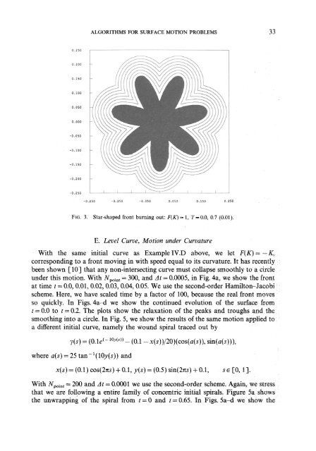
FIG. 3. Star-shaped front burning out: F(K)= 1, T=O.O, 0.7 (0.01).
E. Level Curve, Motion under Curvature
With the same initial curve as Example IV. above, we let F(K) = -K,
corresponding to a front moving in with speed equ to its curvature. It has recently
been shown [lo] that any non-intersecting curve must collapse smoothly to a circle
under this motion. With Npoint = 300, and At = 0.0005, in Fig. 4a, we show the front
at time t = 0.0, 0.01, 0.02,0.03,0.04,0.05. We use the second-order Hamilton-Iacobi
scheme. Here, we have scaled time by a factor of 100, because the real front moves
so quickly. In Figs. 4a-d we show the continued evolution of the surface fr
t = 0.0 to t = 0.2. The plots show the relaxation of the peaks and troughs and
smoothing into a circle. In Fig. 5, we show the results of the same motion applied to
a different initial curve, namely the wound spiral traced out by
y(s) = (O.le’-‘oy(““- (0.1 - x(s))/20)(cos(a(s)), sin(+))),
where a(s) = 25 tan-l( lOy(s)) and
x(s) = (0.1) cos(27rs) + 0.1, y(s) = (0.5) sin(27rs) + 0.1, SE [O, 1-J
With Npoint = 200 and At = 0.0001 we use the second-order scheme. Again, we stress
that we are following a entire family of concentric initial spirals. Figure 5a shows
the unwrapping of the spiral from t = 0 and t = 0.65, In Figs. 5a-d we show the