Using Excel's Solver - Dist

Using Excel’s
SSoollvveerr

Contents
Page
Answer Complex What-If Questions Using Microsoft Excel Solver . . . . . . . . . . . 1
When to Use Solver
Identifying Key Cells in Your Worksheet
Solver Settings are Persistent
Saving a Model or Scenario
Types of Problems Solver Can Analyze
The Difference between Linear and Non Linear Problems
Working with Microsoft Excel Solver . . . . . . . . . . . . . . . . . . . . . . . . . . . . . . . . . . . 4
Solver Installation
Start Solver
Specify the Target Cell (Objective Function)
Specify the Changing Cells (Decision Variables)
Specify the Constraints
Solve the Problem
What to do with the Solver results
Save the Model
Loading Solver Models
Resetting the Solver
Solver Solutions and Special Reports . . . . . . . . . . . . . . . . . . . . . . . . . . . . . . . . . . . . 7
The Sensitivity Report
The Answer Report
The Limits Report
Microsoft Excel Solver Tips and Troubleshooting . . . . . . . . . . . . . . . . . . . . . . . . 10
When Changing Cells and the Target Cell Differ in Magnitude
Mathematical Approaches Used by Solver
When Solver Finds a Solution
When Solver Stops Before a Solution is Found
Starting from Different Initial Solutions

A Case Study Using Microsoft Excel Solver . . . . . . . . . . . . . . . . . . . . . . . . . . . . . 12
Solving a Value to Maximize Another Value
Resetting the Solver Options
Solving for a Value by Changing Several Values
Adding a Constraint
Changing a Constraint
Saving a Problem Model
Microsoft Excel Solver Sample Worksheets . . . . . . . . . . . . . . . . . . . . . . . . . . . . . 16
The Most Profitable Product Mix
The Least Costly Shipping routes
Staff Scheduling at Minimum Cost
Maximizing Income from Working Capital
An Efficient Portfolio of Securities
Further References . . . . . . . . . . . . . . . . . . . . . . . . . . . . . . . . . . . . . . . . . . . . . . . . . 20

Answer Complex What-If Questions Using
Microsoft Excel Solver
Page 1
Excel Solver
Microsoft Excel Solver is a powerful optimization and resource allocation tool. It
can help you determine the best uses of scarce resources so that desired goals such
as profit can be maximized or undesired goals such as cost can be minimized.
Solver answers questions such as:
• What product price or promotion mix will maximize profit?
• How can I live within the budget?
• How fast can we grow without running out of cash?
Instead of guessing over and over, you can use Microsoft Excel Solver to find the
best answers.
When to Use Solver
Use Solver when you need to find the optimum value for a particular cell by
adjusting the values of several cells, or when you want to apply specific limitations
to one or more of the values involved in the calculation.
If you want to find a specific value for a particular cell by adjusting the value of
only one other cell, you can also use the Goal Seek command. For information
about the Goal Seek command, see Microsoft Excel Help for “Goal Seek”.
Identifying Key Cells in Your Worksheet
To use Microsoft Excel Solver with your worksheet model, you define a problem
that needs to be solved by identifying a target cell, the changing cells, and the
constraints that you want used in the analysis.
After you define the problem and start the solution process. Solver finds values
that satisfy the constraints and produce the desired value for the target cell. Solver
then displays the resulting values on your worksheet.
• The target cell (also called the objective or objective function) is the cell in
your worksheet model that you want to minimize, maximize, or set to a certain
value.
• The changing cells (also called decision variables) are cells that affect the
value of the target cell. Solver adjusts the values of the changing cells until a
solution is found.
• A constraint is a cell value that must fall within certain limits or satisfy target
values. Constraints may be applied to the target cell and the changing cells.
Once these items are specified, you are ready to solve the problem. You can
optionally adjust other parameters that control the reporting options, precision, and
mathematical approach used to arrive at a solution.

1
2
3
4
5
6
7
8
9
10
11
12
13
14
15
16
17
18
19
A B C D E F
Quick Tour of Microsoft Excel Solver
Month Q1 Q2 Q3 Q4 Total
Seasonality 0.9 1.1 0.8 1.2
Units Sold 3,592 4,390 3,192 4,789 15,962
Sales Revenue $143,662 $175,587 $127,700 $191,549 $638,498
Cost of Sales 89,789 109,742 79,812 119,718 399,061
Gross Margin 53,873 65,845 47,887 71,831 239,437
Salesforce 8,000 8,000 9,000 9,000 34,000
Advertising 10,000 10,000 10,000 10,000 40,000
Corp Overhead 21,549 26,338 19,155 28,732 95,775
Total Costs 39,549 44,338 38,155 47,732 169,775
Prod. Profit $14,324 $21,507 $9,732 $24,099 $69,662
Profit Margin 10% 12% 8% 13% 11%
Product Price $40.00
Product Cost $25.00
Page 2
Changing cells
Excel Solver
Constraint
Target cell
Solver Settings Are Persistent
After you define a problem, Solver retains the settings you entered in the Solver
Parameters and Solver Options dialog boxes. In a workbook, you can define
separate problems on different sheets, and Solver retains the settings you made for
each sheet individually. The next time you open the workbook and start Solver, the
settings for each appear automatically. You can also try different settings for a
problem on a sheet and save each different group of settings as a model.
Saving a Model or Scenario
After a solution is found, you can choose to save the current settings as a model
using the Save Model button in the Solver Options dialog box.
Saving a model saves the target cell, changing cells, constraints, and Solver Option
settings in a range of cells on the worksheet. Each sheet in a workbook can contain
a different Solver problem, with as many different models as you want for each
problem. Once saved, you can easily load a model by specifying the cell range
where it was saved in the Load Model dialog box.
If you use multiple models, you may want to use the Scenario Manager. The
changing cells you specify with the Scenario Manager will be suggested
automatically as the changing cells in Solver. You can save multiple scenarios for
each worksheet using the Save Scenario button in the Solver Results dialog box.

Types of Problems Solver Can Analyze
The three types of optimization problems that the Solver can analyze are:
• Linear
• Nonlinear
• Integer
Page 3
Excel Solver
Linear and nonlinear optimization problems reflect the nature of the relationships
between elements of the problem as expressed in formulas on your worksheet. If
you know that the problem you are trying to solve is a linear optimization problem
or a linear system of equations and inequalities, you can greatly enhance the
solution process by selecting the Assume Linear Model check box in the Solver
Options dialog box. This is particularly important if your problem is large and
takes a long time to solve.
Integer problems are created by applying an integer constraint to any changing cell
of the problem using the Solver. Use integer constraints when a changing cell used
in the problem must be yes or no (1 or 0), or when decimal values are not desired
(calculating number of employees, for example). Keep in mind that using the
integer method can greatly increase the time necessary for Solver to reach a
solution.
The Difference Between Linear and Nonlinear Problems
A majority of optimization problems involve linear relationship between variables.
A linear relationship would be represented by a straight line on a graph. These
include problems using simple arithmetic operations, such as:
• Addition and subtraction;
• Built-in functions such as SUM().
A problem becomes nonlinear when one or more elements share a disproportional
relationship to one another. A nonlinear problem would be represented by a curved
line on a graph. This can happen when:
• Pairs of changing cells are divided or multiplied by one another;
• Exponentiation is used in the problem;
• You use built-in functions such as GROWTH(), SQRT(), and all
logarithmic functions.

Working with Microsoft Excel Solver
Page 4
Excel Solver
Solver Installation
The Solver macro is an add-in, a supplemental program that adds custom
commands and features to Microsoft Excel. If the Solver command appears on the
Tools menu, it is already installed.
If the Solver command doesn’t appear,
choose the Add-ins command from the
Tools menu to see the list of add-ins
currently available. If Solver appears
there, make sure that its adjacent check
box is selected. If Solver does not
appear, you need to run the Microsoft
Excel Setup program to install the
Solver add-in.
Start Solver
Start by opening the worksheet model you want to use and then choose Solver from
the Tools menu.
Specify the Target Cell (Objective Function)
In the Set Target Cell box, enter the reference or name of the cell you want to
minimize, maximize or set to a certain value.
• The Target cell should contain a formula that depends, directly or indirectly, on
the changing cells you specify in the By Changing Cells box.
• If the target cell does not contain a formula, it must also be a changing cell
• If you don’t specify a target cell, Solver seeks a solution (adjusts values for the
changing cells) that satisfies all of the constraints
Specify the Changing Cells (Decision Variables)
Changing cells normally contain the key variables of your model whose values you
are free to set, such as product prices, amounts to invest, or quantities of a good to
produce. Enter in the By Changing Cells box the references or names of the cells
you want changed by Solver until the constraints in the problem are satisfied and
the target cell reaches its goal.

Page 5
Excel Solver
• If you want Solver to propose the changing cells based on the target cell,
choose the Guess button. If you use the Guess button, you must specify a
target cell.
• You can specify up to 200 changing cells
• Entries in the Changing Cells box consist of a reference to a range of cells, or
references of several nonadjacent cells separated by commas.
Caution If your changing cells contain formulas, Solver will replace them with
constant values if you choose to keep the solution.
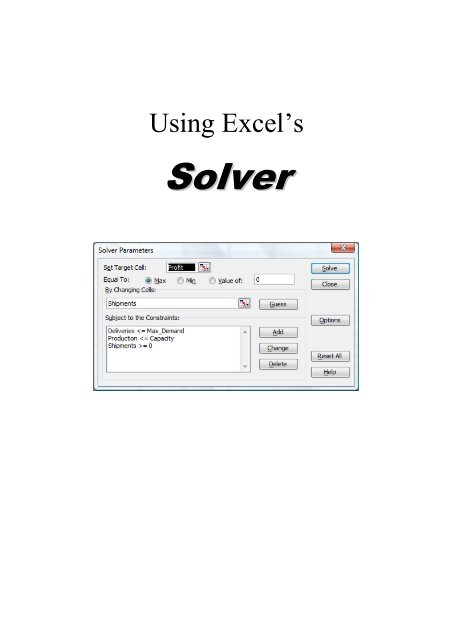
Specify the Constraints
Using the Add, Change and Delete buttons in the Solver Parameters dialog box,
build your list of constraints in the Subject to the Constraints box.
Constraint operator
Cell or range reference or name
Constraint value, formula,
or cell reference
• Constraints can include upper and lower bounds for any cell in your model
including the target cell and the changing cells.
• The cell referred to in the Cell Reference box usually contains a formula that
depends, directly or indirectly, on one or more of the cells you specify as
changing cells.
• When you use the “int” operator, the constrained value is limited to whole
numbers (integers) only. When using integer constraints, you can use the
Tolerance setting in the Solver Options dialog box to adjust the allowable
margin of error.
• When you use the “bin” operator, the constrained value is limited to binary
values 0 and 1 only.
• Only changing cells can be restricted to integer or binary values.
• For each problem, you can specify two constraints for each changing cell (one
upper-limit and one lower-limit constraint), plus up to 200 additional
constraints.
Fore more information about integer constraints and the Tolerance setting, see
“Microsoft Excel Solver Tips and Troubleshooting” later in this document.

Solve the Problem
Pressing the Solve button initiates the problem-solving process.
Problem solution difficulty depends on:
Page 6
Excel Solver
• The size of the model, that is, the number of decision variables and constraints
• The mathematical relationships between the objective and constraints, and the
decision variables
• The use of integer constraints
Solver’s solution process involves successive trials, or iterations. During each
iteration, Solver uses a new set of changing cell values to recalculate the
worksheet, and examines the constraints and optimum cell values. The process
stops when a solution is found to acceptable precision, no further progress is
possible, or the maximum time allowed or the maximum number of iterations is
reached (see the Solver Options dialog box).
What to Do with the Solver Results
When the problem-solving process ends, a dialog box displays several choices.
You can:
• Keep the solution Solver found, or restore the original values in your
worksheet;
• Save the solution as a named scenario using the Scenario Manager;
• View any of Solver’s built-in reports.
Save the model
You can save your model’s settings (cell selections, constraints and options) by
choosing the Save Model button in the Solver Options dialog box. When you save
a model, Microsoft Excel stores its settings as a range of cells containing formulas.
While the latest Solver settings are automatically displayed the next time you open
the worksheet, you can save many different models using the Save Model button.
1
2
3
4
5
6
7
8
9
10
11
12
13
14
15
16
17
A B C D E F G H I
Quick Tour of Microsoft Excel Solver
Month Q1 Q2 Q3 Q4 Total
Seasonality 0.9 1.1 0.8 1.2
Units Sold 3,592 4,390 3,192 4,789 15,962
Sales Revenue $143,662 $175,587 $127,700 $191,549 $638,498
Cost of Sales 89,789 109,742 79,812 119,718 399,061 $69,662
Gross Margin 53,873 65,845 47,887 71,831 239,437 4
TRUE
Salesforce 8,000 8,000 9,000 9,000 34,000 100
Advertising 10,000 10,000 10,000 10,000 40,000
Corp Overhead 21,549 26,338 19,155 28,732 95,775
Total Costs 39,549 44,338 38,155 47,732 169,775
Prod. Profit $14,324 $21,507 $9,732 $24,099 $69,662
Profit Margin 10% 12% 8% 13% 11%
Model saved
on worksheet
Solver saves a model in a range starting with the cell you specify in the Save Model
dialog box. The size of the range depends on the number of constraints you specify.

Page 7
Excel Solver
Tip Naming each model range that you save makes it easier to remember your
models and load them later
Loading Solver Models
To replace the current Solver settings with a set of saved settings, choose the Load
Model button in the Solver Options dialog box, and enter the name or reference of
the range containing the settings you want to load.
Resetting the Solver
If you apply Solver to a problem previously undefined in Solver on a new sheet,
the settings of the Solver Parameters dialog box appear in their default state.
However, for the Solver Options dialog box, any settings you used during your
current Microsoft Excel session remain in effect. You can easily reset them using
the Reset All button in the Solver Parameters dialog box.
Solver Solutions and Special Reports
Using Microsoft Excel Solver, you can create three types of reports that summarize
the results of the successful solution process.
Microsoft Excel creates each report on a separate sheet in the current workbook.
To print the report, switch to the sheet containing the report, and choose the Print
command from the File menu.
The Sensitivity Report
The Sensitivity report contains information demonstrating how sensitive a solution
is to changes in the formulas used in the problem. There are two versions of this
report, depending on whether you selected the Assume Linear Model option in the
Solver Options dialog box.

Microsoft Excel 10.0 Sensitivity Report
Worksheet: [Solvsamp.xls]Product Mix
Report Created: 2/12/2004 20:29:17
Adjustable Cells
Final Reduced
Cell Name Value Gradient
$D$9 Number to Build-> TV set 160 0
$E$9 Number to Build-> Stereo 200 0
$F$9 Number to Build-> Speaker 80 0
Constraints
Final Lagrange
Cell Name Value Multiplier
$C$11 Chassis No. Used 360 0
$C$12 Picture Tube No. Used 160 0
$C$13 Speaker Cone No. Used 800 6
$C$14 Power Supply No. Used 360 0
$C$15 Electronics No. Used 600 14
Sensitivity report for nonlinear problems
Page 8
Excel Solver
• Reduced Gradient Measures the increase in the target cell per unit increase
in the changing cell.
• Lagrange Multiplier Measures the increase in the target cell per unit
increase of the corresponding constraint.
A different version of the Sensitivity report is generated if you select the Assume
Linear Model check box in the Solver Options dialog box.
Microsoft Excel 10.0 Sensitivity Report
Worksheet: [Solvsamp.xls]Product Mix
Report Created: 2/12/2004 20:36:34
Adjustable Cells
Final Reduced Objective Allowable Allowable
Cell Name Value Cost Coefficient Increase Decrease
$D$9 Number to Build-> TV set 200 0 75 25 5.0
$E$9 Number to Build-> Stereo 200 0 50 25 12.5
$F$9 Number to Build-> Speaker 0 -2.50 35 2.5 1E+30
Constraints
Final Shadow Constraint Allowable Allowable
Cell Name Value Price R.H. Side Increase Decrease
$C$11 Chassis No. Used 400 0.0 450 1E+30 50
$C$12 Picture Tube No. Used 200 0.0 250 1E+30 50
$C$13 Speaker Cone No. Used 800 12.5 800 100 100
$C$14 Power Supply No. Used 400 0.0 450 1E+30 50
$C$15 Electronics No. Used 600 25.0 600 50 200
Sensitivity report for linear problems
This version of the Sensitivity report adds the following information for each
changing cell:

Page 9
Excel Solver
• Reduced Cost Replaces reduced Gradient, and measures the increase in the
target cell per unit increase in the changing cell.
• Objective Coefficient Measures the relative (linear) relationship between a
changing cell and the target cell.
• Allowable Increase Shows the increase in the objective coefficient before
there would be a change in the optimal value of any of the changing cells.
• Allowable Decrease Shows the decrease in the objective coefficient before
there would be a change in the optimal value of any of the changing cells.
The following information is added for each constraint cell:
• Shadow Price Replaces Lagrange Multiplier, and measures the increase in
the objective per unit increase in the right side of the constraint equation.
• Constraint RH Side (right-hand side) Lists the constraint values you
specified.
• Allowable Increase Shows the increase in the Constraint RH Side value
before there would be a change in the Shadow Price.
• Allowable Decrease Shows the decrease in the Constraint RH Side value
before there would be a change in the Shadow Price.
The Answer Report
This report shows:
• The target cell (entered in the Set Target Cell box in the Solver Parameters
dialog box).
• The changing cells, with their original and final values.
• The constraints and information about them.
Microsoft Excel 10.0 Answer Report
Worksheet: [Solvsamp.xls]Product Mix
Report Created: 2/12/2004 20:42:06
Target Cell (Max)
Cell Name Original Value Final Value
$D$18 Total Profits: $10,095 $14,917
Adjustable Cells
Cell Name Original Value Final Value
$D$9 Number to Build-> TV set 100 160
$E$9 Number to Build-> Stereo 100 200
$F$9 Number to Build-> Speaker 100 80
Constraints
Cell Name Cell Value Formula Status Slack
$C$11 Chassis No. Used 360 $C$11 Speaker 80 $F$9>=0 Not Binding 80.21
Information about constraints appears in the Status and Slack columns. These
columns tell you how each constraint was met.

In the Status column, one of the following values is displayed.
Page 10
Excel Solver
• Binding The final cell value equals the constraint value. For example, if the
constraint is C11 Speaker 80 0 13107 80 14917
• Lower Limit The smallest value that a changing cell can take while holding
all the other changing cells fixed and still satisfying the constraints.
• Upper Limit The greatest value that a changing cell can take while holding
all the other changing cells fixed and still satisfying the constraints.
• Target result The value of the target cell when the changing cell is at its
lower or upper limit.
Microsoft Excel Solver Tips and Troubleshooting
When Changing Cells and the Target Cell
Differ in Magnitude
To find a solution to a problem involving changing cells that differ from the target
cell by more than one order of magnitude, select the Use Automatic Scaling check
box in the Solver Options dialog box. For example, you would select this option if
you were planning to invest $10,000,000 in five different stocks and were trying to
find the best return on the investment. The changing cells would be in the tens of

Page 11
Excel Solver
millions, and the target cell would be a percentage value, eight or nine orders of
magnitude smaller than the changing cells.
Mathematical Approaches Used by Solver
You can use the boxes at the bottom of the Solver Options dialog box to choose
among alternative technical approaches used by Solver at various points in the
solution process. The default settings for these options are suitable for nearly all
problems. Use of these options is primarily for those experienced in mathematical
optimization methods: if you’re having difficulty reaching the optimal solution you
want, you can experiment with these options in an effort to obtain better results.
When Solver Finds a Solution
Solver will display one of the following messages when it has found a solution to
your problem.
• Solver found a solution All constraints and optimality conditions are
satisfied. All constraints are satisfied to within the precision and integer
tolerance settings, and, if appropriate, a maximum, minimum, or target value
has been found for the cell in the Set target Cell box.
• Solver has converged to the current solution All constraints are satisfied.
The value in the cell named in the set Target Cell box is virtually unchanged
for the last five trial solutions. A solution may have been found, but it is also
possible that the iterative solution process is making very slow progress and is
far from a solution, that the Precision setting (set with the Precision box in the
Solver Options dialog box) is too low, or that the initial values for the changing
cells were too far from the solution.
When Solver Stops Before a Solution Is Found
While solving a problem, Solver may stop before an optimal solution or even a
feasible solution has been found. If this happens, a dialog box with one of the
Solver completion messages will appear, and you’ll have the choice of keeping the
latest values of the changing cells or restoring their former contents.
Some of the reasons this may happen:
• You interrupted the solution process (e.g., by pressing the Esc key).
• You chose the Stop button while stepping through iterations.
• You chose the Stop button when the maximum time or maximum number of
iterations was reached.
• The Set Target cell value is increasing or decreasing without limit.
• The Assume Linear Model option is selected when the problem is nonlinear.
• You have a complex model containing integer constraints, and you need to
adjust the tolerance setting to a higher percentage or increase the Max Time or
Iterations setting.
• You need to select the Automatic Scaling option because some input values are
several orders of magnitude apart, or input values are different from output
values by several orders of magnitude.

Page 12
Excel Solver
Starting from Different Initial Solutions
The ultimate solution can depend on the initial values you supply for the changing
cells. Setting the changing cells to values that you suspect are close to optimal can
often reduce the solution time. This is especially important if you select the Use
Automatic Scaling option or if you have applied integer constraints. If Solver finds
a solution that is very different from what you expected, try rerunning Solver with
different starting values for the changing cells.
A Case Study Using Microsoft Excel Solver
This section takes you on a quick tour of Microsoft Excel Solver’s features. The
sample worksheet used in this section is in a workbook called SOLVSAMP.XLS,
available within a folder where Microsoft Excel is located, typically:
C:\Program Files\Microsoft Office\Office11\Samples\. The file SOLVSAMP.XLS
is also available in the electronic course material, either on website or CD-ROM.
You can open the workbook and solve several problems by following the examples
in this section. In this process, you’ll learn how to:
• Solve for one value or several values to maximize or minimize another value.
• Enter and change constraints.
• Save a problem model.
The following illustration shows the Solver sample worksheet.
1
2
3
4
5
6
7
8
9
10
11
12
13
14
15
16
17
18
19
A B C D E F G
Quick Tour of Microsoft Excel Solver
Month Q1 Q2 Q3 Q4 Total
Seasonality 0.9 1.1 0.8 1.2
Units Sold 3,592 4,390 3,192 4,789 15,962
Sales Revenue $143,662 $175,587 $127,700 $191,549 $638,498
Cost of Sales 89,789 109,742 79,812 119,718 399,061
Gross Margin 53,873 65,845 47,887 71,831 239,437
Salesforce 8,000 8,000 9,000 9,000 34,000
Advertising 10,000 10,000 10,000 10,000 40,000
Corp Overhead 21,549 26,338 19,155 28,732 95,775
Total Costs 39,549 44,338 38,155 47,732 169,775
Prod. Profit $14,324 $21,507 $9,732 $24,099 $69,662
Profit Margin 10% 12% 8% 13% 11%
Product Price $40.00
Product Cost $25.00

Row Contains Explanation
Page 13
Excel Solver
3 Fixed values Seasonality factor: sales are higher in quarters 2 and
4, and lower in quarters 1 and 3
5 =35*B3*(B11+3000)^0.5 Forecast for units sold each quarter: row 3 contains
the seasonality factor; row 11 contains the cost of
advertising
6 =B5*$B$18 Sales revenue: forecast for units sold (row 5) times
price (cell B18)
7 =B5*$B$19 Cost of sales: forecast for units sold (row 5) times
product cost (cell B19)
8 =B6-B7 Gross margin: sales revenues (row 6) minus cost of
sales (row 7)
10 Fixed values Sales personnel expenses
11 Fixed values Advertising budget
12 =0.15*B6 Corporate overhead expenses: sales revenues (row 6)
times 15%
13 =SUM(B10:B12) Total costs: sales personnel expenses (row 10) plus
advertising (row 11) plus overhead (row 12)
15 =B8-B13 Product profit: gross margin (row 8) minus total
costs (row 13)
16 =B15/B6 Profit margin: profit (row 15) divided by sales
revenue (row 6)
18 Fixed values Product price
19 Fixed values Product cost
This is a typical marketing model that shows sales rising from a base figure
(perhaps due to the sales personnel) along with increases in advertising, but with
diminishing returns. For example, the first $5000 of advertising in Q1 yields about
1092 incremental units sold, but the next $5000 yields only about 775 units more.
You can use Solver to find out whether the advertising budget is too low, and
whether advertising should be allocated differently over time to take advantage of
the changing seasonality factor.
Solving for a Value to Maximize Another Value
One way you can use Solver is to determine the maximum value of a cell by
changing another cell. The two cells must be related through the formulas on the
worksheet. If they are not, changing the value in one cell will not change the value
in the other cell.

Page 14
Excel Solver
For example, in the sample worksheet, you want to know how much you need to
spend on advertising to generate the maximum profit for the first quarter. You are
interested in maximizing profit by changing advertising expenditures.
• From the Tools menu, choose Solver. In the Set Target Cell box, type b15 or
select cell B15 (first-quarter profits) on the worksheet. Select the Max option
button. In the By Changing Cells box, type b11 or select B11 (first-quarter
advertising) on the worksheet. Choose the Solve button.
You will see messages in the status bar as the problem is set up and Solver starts
working. After a moment, you’ll see a message that Solver has found a solution.
Solver finds that Q1 advertising of $17,093 yields the maximum profit $15,093.
• After you examine the results, select the Restore Original values option button
and choose the OK button to discard the results and return cell B11 to its
former value.
Resetting the Solver Options
If you want to return the options in the Solver Parameters dialog box to their
original settings so that you can start a new problem, you can use the Reset All
button.
Solving for a Value by Changing Several Values
You can also use Solver to solve for several values at once to maximize or
minimize another value. For example, in the sample worksheet, you can solve for
the advertising budget for each quarter that will result in the best profits for the
entire year. Since the seasonality factor in row 3 enters into the calculation of unit
sales in row 5 as a multiplier, it seems logical that you should spend more of your
advertising budget in Q4 when the sales response is highest, and less in Q3 when
the sales response is lowest. Use Solver to determine the best quarterly allocation.
• From the Tools menu, choose Solver. In the Set target Cell box, type f15 or
select cell F15 (total profits for the year) on the worksheet. Make sure the Max
option button is selected. In the By Changing Cells box, type b11:e11 or select
cells B11:E11 (the advertising budget for each of the four quarters) on the
worksheet. Choose the Solve button.
• After you examine the results, select the Restore Original Values option button
and choose the OK button to discard the results and return all cells to their
former values.
You’ve just asked Solver to solve a moderately complex nonlinear optimization
problem – that is, to find values for the four unknowns in cells B11 through E11
that will maximize profits. (This is a nonlinear problem because of the
exponentiation that occurs in the formulas in row 5.) The results of this
unconstrained optimization show that you can increase profits for the year to
$79,706 if you spend $89,706 in advertising for the full year.

Page 15
Excel Solver
However, most realistic modeling problems have limiting factors that you will
want to apply to certain values. These constraints may be applied to the target cell,
the changing cells or any other value that is related to the formulas in these cells.
Adding a Constraint
So far, the budget recovers the advertising cost and generates additional profit, but
you’re reaching a point of diminishing returns. Since you can never be sure that
your model of sales response to advertising will be valid next year (especially at
greatly increased spending levels), it doesn’t seem prudent to allow unrestricted
spending on advertising.
Suppose you want to maintain your original advertising budget of $40,000. Add
the constraint to the problem that limits the sum of advertising during the four
quarters to $40,000.
• From the Tools menu, choose Solver. Choose the Add button. The Add
Constraint dialog box appears. In the Cell Reference box, type f11 or select
cell F11 (advertising total) on the worksheet. Cell F11 must be less than or
equal to $40,000. The relationship in the Constraint box is “

Page 16
Excel Solver
Saving a Problem Model
When you choose Save from the File menu, the last selections made in the Solver
Parameters dialog box are attached to the worksheet and retained when you save
the workbook. However, you can define more than one problem for a worksheet
by saving them individually using the Save Model button in the Solver Options
dialog box. Each problem model consists of cells and constraints that you entered
in the Solver Parameters dialog box.
When you choose the Save Model button, the Save Model dialog box appears with
a default selection, based on the active cell, as the area for saving the model. The
suggested range includes a cell for each constraint plus three additional cells.
Make sure that this cell range is an empty range on the worksheet.
• From the Tools menu, choose Solver. Choose the Options button. Choose the
Save Model button. In the Select Model Area box, type c17:c20 or select cells
C17:C20 on the worksheet. Choose the OK button.
Note You can also enter a reference to a single cell in the Select Model Area box.
Solver will use this reference as the upper-left corner of the range into which it will
copy the problem specifications.
To load these problem specifications later, choose the Load Model button in the
Solver Options dialog box, then type c17:c20 in the Model Area box or select cells
C17:C20 on the sample worksheet and choose the OK button. Solver displays a
message asking if you want to reset the current Solver option settings with the
settings for the model you are loading. Choose the OK button to proceed.
Microsoft Excel Solver Sample Worksheets
This section gives brief introductory information about the sample worksheets
included for use with Solver.
The sample worksheets are available in the SOLVSAMP.XLS workbook typically
located in a folder within the directory where Microsoft Excel is located. This file
is also available among the electronic material supplied for the course.
When you open this workbook, and then switch to one of the worksheets and
choose the Solver command, you will see that the target cell, changing cells, and
constraints are already specified for that worksheet.
The Most Profitable Product Mix
The sample worksheet named Product Mix provides data for several products using
common parts, each with a different profit margin per unit. Parts are limited, so
your problem is to determine the number of each product to build from the
inventory on hand in order to maximize profits.

Problem Specifications
Page 17
Excel Solver
Target cell D18 Goal is to maximize profit
Changing cells D9:F9 Units of each product to build
Constraints C11:C15=0 Number to build value must be
greater than or equal to 0
The formulas for profit per product in cells D17:F17 include the factor ^H15 to
show that profit per unit diminishes with volume. H15 contains 0.9 which makes
the problem nonlinear. If you change H15 to 1.0 to indicate that profit per unit
remains constant with volume, and then choose the Solve button again, the optimal
solution will change. This change also makes the problem linear.
The Least Costly Shipping Routes
The problem presented on the sample worksheet named Shipping Routes involves
the shipment of goods from three plants to five regional warehouses. Goods can be
shipped from any plant to any warehouse, but it obviously costs more to ship goods
over long distances than over short distances. The problem is to determine the
amounts to ship from each plant to each warehouse at minimum shipping cost in
order to meet the regional demand, while not exceeding the plant supplies.
Problem Specifications
Target cell B20 Goal is to minimize total
shipping cost
Changing cells C8:G10 Amount to ship from each plant
to each warehouse
Constraints B8:B10=C14:G14 Totals shipped to warehouses
must be greater than or equal to
demand at warehouses
C8:G10>=0 Number to ship must be greater
than or equal to 0
You can solve this problem faster by selecting the Assume Linear Model check
box in the Solver options dialog box before choosing the Solve button. A problem
of this type will have an optimum solution in which amounts to ship are integers, if
all of the supply and demand constraints are integers.
Staff Scheduling at Minimum Cost
The goal for the sample worksheet named Staff Scheduling is to schedule
employees so that you have sufficient staff at the lowest cost. In this example, all
employees are paid at the same rate, so by minimizing the number of employees
working each day, you also minimize costs. Each employee works five
consecutive days, followed by two days off.

Problem Specifications
Page 18
Excel Solver
Target cell D20 Goal is to minimize payroll cost
Changing cells D7:D13 Employees on each schedule
Constraints D7:D13>=0 Number of employees must be
greater than or equal to 0
D7:D13=Integer Number of employees must be
an integer
F15:L15>=F17:L17 Employees working each day
must be greater than or equal to
the demand
Possible schedules Rows 7-13 1 means employee on that
schedule works that day
In this example, you use an integer constraint so that your solutions do not result in
fractional numbers of employees on each schedule. Selecting the Assume Linear
Model check box in the Solver Options dialog box before you choose the Solve
button will greatly speed up the solution process.
Maximizing Income from Working Capital
If you’re a financial officer or a manager, one of your tasks is to manage cash and
short-term investments in a way that maximizes interest income, while keeping
funds available to meet expenditures. You must trade off the higher interest rates
available from longer-term investments against the flexibility provided by keeping
funds in short-term investments.
The sample worksheet named Maximizing Income calculates ending cash based on
initial cash (from the previous month), inflows from maturing certificates of
deposit (CDs), outflows for new CDs, and cash needed for company operations for
each month.
You have a total of nine decisions to make : the amounts to invest in one-month
CDs in months 1 through 6 ; the amounts to invest in three-month CDs in months 1
and 4 ; and the amount to invest in six-month CDs in month 1.
Problem Specifications
Target cell H8 Goal is to maximize interest
earned
Changing cells B14:G14
B15, E15, B16
Constraints B14:G14>=0
B15:B16>=0
E15>=0
B18:H18>=100000
Amount to invest B11 $400,000
Cash use aside from
investments
Row 17
Dollars invested in each type
of CD
Investment in each type of
CD must be greater than or
equal to 0
Ending cash must be greater
than or equal to $100,000

Page 19
Excel Solver
The optimal solution determined by Solver earns a total interest income of $16,531
by investing as much as possible in six-month and three-month CDs and then turns
to one-month CDs. This solution satisfies all of the constraints.
Suppose, however, that you want to guarantee that you have enough cash in month
5 for an equipment payment. Add a constraint that the average maturity of the
investments held in month 1 should not be more than four months.
The formula in cell B20 computes a total of the amounts invested in month 1 (B14,
B15 and B16) weighted by the maturities (1, 3 and 6 months), and then it subtracts
from this amount the total investment, weighted by 4. If this quantity is zero or
less, the average maturity will not exceed four months. To add this constraint,
choose Solver from the Tools men, then choose the Add button. Type b20 in the
cell Reference box, type 0 in the Constraint box, and then choose the OK button.
To solve the problem, choose the Solve button.
To satisfy the four-month maturity constraint, Solver shifts funds from six-month
CDs to three month CDs. The shifted funds now mature in month 4 and, according
to the present plan, are reinvested in new three-month CDs. If you need the funds,
however, you can keep the cash instead of reinvesting. The $56,896 turning over
in month 4 is more than sufficient for the equipment payment in month 5. You’ve
traded about $460 in interest income to gain this flexibility.
An Efficient Portfolio of Securities
One of the basic principles of investment management is diversification. By
holding a portfolio of several stocks, for example, you can earn a rate of return that
represents the average of the returns from the individual stocks, while reducing
your risk that any one stock will perform poorly.
Using the sample worksheet named Portfolio of securities, you can use Solver to
find the allocation of funds to stocks that minimizes the portfolio risk for a given
rate of return, or that maximizes the rate of return for a given level of risk.
This worksheet contains figures for beta (market-related risk) and residual variance
for four stocks. In addition, your portfolio includes investments in treasury bills
(T-bills), assumed to have a risk-free rate of return and a variance of zero. Initially,
equal amounts (20 percent of the portfolio) are invested in each security.
Use solver to try different allocations of funds to stocks and T-bills to either
maximize the portfolio rate of return for a specified level of risk or minimize the
risk for a given rate of return. With the initial allocation of 20 percent across the
board, the portfolio return is 16.4 percent and the variance is 0.071.

Page 20
Excel Solver
Problem Specifications
Target cell E18 Goal is to maximize Portfolio
return
Changing cells E10:E14 Weight of each stock
Constraints E10:E14>=0 Weights must be greater than or
equal to 0
E16=1 Sum of weights must equal 1
G18