The Nucleon-Nucleon Interaction in a Chiral Effective Field Theory

3.8. Two-nucleon potential 93
topological aspects of the processes. Different to time-ordered perturbation theory, one cannot
directly read off the corresponding matrix element from the diagram. To do that, one has to insert
the appropriate energy denominators from eqs. (3.253)-(3.255).
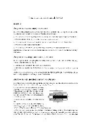
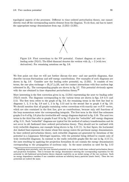
Figure 3.8: First corrections to the NN potential. Contact diagram at next-toleading
order (NLO). The filled diamond denotes the vertices with L::.i = 2 (with two
derivatives). For remaining notations see fig. 3.6.
We first point out that we will not furt her discuss the zero- arid one-particle diagrams, that
describe vacuum fiuctuations and self-energy contributions. Few examples of such diagrams are
shown in fig. 3.6. Consider now the leading order potential, eq. (3.253). It consists of two
terms, the one-pion exchange rv H1 ().. 1 /w)H1 and the contact interactions with four nucleon legs
subsumed in H2 . The corresponding graphs are shown in fig. 3.7. This potential obviously agrees
with the one obtained in time-dependent perturbation theory.40
More interesting is the first correction given in eq. (3.254) representing the next-to-leading order
(NLO) result. The diagrams corresponding to the various terms are shown in figs. 3.8-3.11 and
3.13. The first term refers to the graph of fig. 3.8, the remaining terms in the first line lead to
diagrams 1, 2, 3 in fig. 3.9 and 1, 2 in fig. 3.13 and in the second line to graph 4 of fig. 3.9.
We should mention that all graphs containing vertex corrections with exactly one 7r7r N N -vertex,
which are also contained in the first line, give no contributions, because only odd functions of
the loop moment um enter the corresponding integrals. The first term in the third line subsumes
graphs 5 to 8 offig. 3.9 plus the irreducible self-energy diagrams depicted in fig. 3.10. The next two
terms in the third line refer to graphs 9 and 10 in fig. 3.9 plus the "reducible" self-energy diagrams
offig. 3.11. Such "reducible" diagrams are typical for the method ofunitary transformation and do
not occur in old-fashioned time-ordered perturbation theory. They should not be confused with
truly reducible diagrams, one example being shown in fig. 3.12 (1). In that figure, the horizontal
dot-dashed lines represent the states whose free energy enters the pertinent energy denominators.
In time-ordered perturbation theory, such reducible diagrams are generated by iterations of the
potential in a Lippmann-Schwinger equation, with the potential being defined to consist only of
truly irreducible diagrams. In contrast to the really reducible graphs like the one in fig. 3.12 (1),
the ones resulting by applying the projection formalism do not contain the energy denominators
corresponding to the propagation of nucleons only. In the same notation as used for fig. 3.12
4° Speaking more precisely, only the non-iterated potential is the same in both time-ordered perturbation theory
and projection formalism. This is because the energy denominator entering the corresponding expression for the
potential in old-fashioned perturbation theory depends explicitly on an initial energy of the two nucleons. Such
an energy dependence vanishes if one considers nucleons as infinitely heavy particles (static limit). Then the two
potentials are indeed the same.