fluid_mechanics

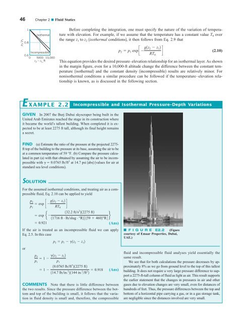
46 Chapter 2 ■ Fluid Statics
p 2 /p 1
1
0.8
Isothermal
Incompressible
0.6
0 5000 10,000
z 2 – z 1, ft
Before completing the integration, one must specify the nature of the variation of temperature
with elevation. For example, if we assume that the temperature has a constant value T 0 over
the range z 1 to z 2 1isothermal conditions2, it then follows from Eq. 2.9 that
p 2 p 1 exp c g1z 2 z 1 2
d
RT 0
(2.10)
This equation provides the desired pressure–elevation relationship for an isothermal layer. As shown
in the margin figure, even for a 10,000-ft altitude change the difference between the constant temperature
1isothermal2 and the constant density 1incompressible2 results are relatively minor. For
nonisothermal conditions a similar procedure can be followed if the temperature–elevation relationship
is known, as is discussed in the following section.
E XAMPLE 2.2
Incompressible and Isothermal Pressure–Depth Variations
GIVEN In 2007 the Burj Dubai skyscraper being built in the
United Arab Emirates reached the stage in its construction where
it became the world’s tallest building. When completed it is expected
to be at least 2275 ft tall, although its final height remains
a secret.
FIND (a) Estimate the ratio of the pressure at the projected 2275-
ft top of the building to the pressure at its base, assuming the air to be
at a common temperature of 59 °F. (b) Compare the pressure calculated
in part (a) with that obtained by assuming the air to be incompressible
with g 0.0765 lbft 3 at 14.7 psi 1abs2 1values for air at
standard sea level conditions2.
SOLUTION
For the assumed isothermal conditions, and treating air as a compressible
fluid, Eq. 2.10 can be applied to yield
If the air is treated as an incompressible fluid we can apply
Eq. 2.5. In this case
or
p 2
exp c g1z 2 z 1 2
d
p 1 RT 0
132.2 fts 2 212275 ft2
exp e
11716 ft # lbslug # °R23159 4602°R4 f
0.921
(Ans)
p 2 p 1 g1z 2 z 1 2
p 2
1 g1z 2 z 1 2
p 1 p 1
1
10.0765 lb ft 3 212275 ft2
114.7 lbin. 2 21144 in. 2 ft 2 2 0.918
(Ans)
COMMENTS Note that there is little difference between
the two results. Since the pressure difference between the bottom
and top of the building is small, it follows that the variation
in fluid density is small and, therefore, the compressible
F I G U R E E2.2 (Figure
courtesy of Emaar Properties, Dubai,
UAE.)
fluid and incompressible fluid analyses yield essentially the
same result.
We see that for both calculations the pressure decreases by approximately
8% as we go from ground level to the top of this tallest
building. It does not require a very large pressure difference to support
a 2275-ft-tall column of fluid as light as air. This result supports
the earlier statement that the changes in pressures in air and other
gases due to elevation changes are very small, even for distances of
hundreds of feet. Thus, the pressure differences between the top and
bottom of a horizontal pipe carrying a gas, or in a gas storage tank,
are negligible since the distances involved are very small.