fluid_mechanics
42 Chapter 2 ■ Fluid Statics p For liquids or gases at rest, the pressure gradient in the vertical direction at any point in a fluid depends only on the specific weight of the fluid at that point. dz g dp 1 dp ––– = −g dz V2.1 Pressure on a car z change. Since p depends only on z, the last of Eqs. 2.3 can be written as the ordinary differential equation Equation 2.4 is the fundamental equation for fluids at rest and can be used to determine how pressure changes with elevation. This equation and the figure in the margin indicate that the pressure gradient in the vertical direction is negative; that is, the pressure decreases as we move upward in a fluid at rest. There is no requirement that g be a constant. Thus, it is valid for fluids with constant specific weight, such as liquids, as well as fluids whose specific weight may vary with elevation, such as air or other gases. However, to proceed with the integration of Eq. 2.4 it is necessary to stipulate how the specific weight varies with z. If the fluid is flowing (i.e., not at rest with a 0), then the pressure variation is much more complex than that given by Eq. 2.4. For example, the pressure distribution on your car as it is driven along the road varies in a complex manner with x, y, and z. This idea is covered in detail in Chapters 3, 6, and 9. 2.3.1 Incompressible Fluid Since the specific weight is equal to the product of fluid density and acceleration of gravity 1g rg2, changes in g are caused either by a change in r or g. For most engineering applications the variation in g is negligible, so our main concern is with the possible variation in the fluid density. In general, a fluid with constant density is called an incompressible fluid. For liquids the variation in density is usually negligible, even over large vertical distances, so that the assumption of constant specific weight when dealing with liquids is a good one. For this instance, Eq. 2.4 can be directly integrated to yield or p 1 p 2 g1z 2 z 1 2 (2.5) where p 1 and p 2 are pressures at the vertical elevations z 1 and z 2 , as is illustrated in Fig. 2.3. Equation 2.5 can be written in the compact form or p 2 dp dz g z 2 dp g p 1 dz p 2 p 1 g1z 2 z 1 2 p 1 p 2 gh p 1 gh p 2 where h is the distance, z 2 z 1 , which is the depth of fluid measured downward from the location of p 2 . This type of pressure distribution is commonly called a hydrostatic distribution, and Eq. 2.7 z 1 (2.4) (2.6) (2.7) Free surface (pressure = p 0 ) p 2 z h = z 2 – z 1 z 2 p1 x z 1 y F I G U R E 2.3 Notation for pressure variation in a fluid at rest with a free surface.
2.3 Pressure Variation in a Fluid at Rest 43 23.1 ft pA = 0 A = 1 in. 2 = 10 lb Water shows that in an incompressible fluid at rest the pressure varies linearly with depth. The pressure must increase with depth to “hold up” the fluid above it. It can also be observed from Eq. 2.6 that the pressure difference between two points can be specified by the distance h since h p 1 p 2 g In this case h is called the pressure head and is interpreted as the height of a column of fluid of specific weight g required to give a pressure difference p 1 p 2 . For example, a pressure difference of 10 psi can be specified in terms of pressure head as 23.1 ft of water 1g 62.4 lbft 3 2, or 518 mm of Hg 1g 133 kNm 3 2. As illustrated by the figure in the margin, a 23.1-ft-tall column of water with a cross-sectional area of 1 in. 2 weighs 10 lb. pA = 10 lb F l u i d s i n t h e N e w s Giraffe’s blood pressure A giraffe’s long neck allows it to graze up to 6 m above the ground. It can also lower its head to drink at ground level. Thus, in the circulatory system there is a significant hydrostatic pressure effect due to this elevation change. To maintain blood to its head throughout this change in elevation, the giraffe must maintain a relatively high blood pressure at heart level—approximately two and a half times that in humans. To prevent rupture of blood vessels in the high-pressure lower leg regions, giraffes have a tight sheath of thick skin over their lower limbs which acts like an elastic bandage in exactly the same way as do the g-suits of fighter pilots. In addition, valves in the upper neck prevent backflow into the head when the giraffe lowers its head to ground level. It is also thought that blood vessels in the giraffe’s kidney have a special mechanism to prevent large changes in filtration rate when blood pressure increases or decreases with its head movement. (See Problem 2.14.) When one works with liquids there is often a free surface, as is illustrated in Fig. 2.3, and it is convenient to use this surface as a reference plane. The reference pressure p 0 would correspond to the pressure acting on the free surface 1which would frequently be atmospheric pressure2, and thus if we let p 2 p 0 in Eq. 2.7 it follows that the pressure p at any depth h below the free surface is given by the equation: p gh p 0 (2.8) As is demonstrated by Eq. 2.7 or 2.8, the pressure in a homogeneous, incompressible fluid at rest depends on the depth of the fluid relative to some reference plane, and it is not influenced by the size or shape of the tank or container in which the fluid is held. Thus, in Fig. 2.4 Liquid surface (p = p 0 ) h A B Specific weight γ F I G U R E 2.4 Fluid pressure in containers of arbitrary shape.
- Page 15 and 16: Preface xiii WileyPLUS offers today
- Page 17 and 18: Featured in this Book xv LEARNING O
- Page 19 and 20: C ontents 1 INTRODUCTION 1 Learning
- Page 21 and 22: Contents xix 6.4.3 Irrotational Flo
- Page 23: 12.6 Axial-Flow and Mixed-Flow Pump
- Page 26 and 27: 10 8 Jupiter red spot diameter 2 Ch
- Page 28 and 29: 4 Chapter 1 ■ Introduction and do
- Page 30 and 31: 6 Chapter 1 ■ Introduction up the
- Page 32 and 33: 8 Chapter 1 ■ Introduction the SI
- Page 34 and 35: 10 Chapter 1 ■ Introduction E XAM
- Page 36 and 37: 12 Chapter 1 ■ Introduction TABLE
- Page 38 and 39: 14 Chapter 1 ■ Introduction TABLE
- Page 40 and 41: 16 Chapter 1 ■ Introduction Crude
- Page 42 and 43: 18 Chapter 1 ■ Introduction Visco
- Page 44 and 45: 20 Chapter 1 ■ Introduction Kinem
- Page 46 and 47: 22 Chapter 1 ■ Introduction As th
- Page 48 and 49: 24 Chapter 1 ■ Introduction Boili
- Page 50 and 51: 26 Chapter 1 ■ Introduction E XAM
- Page 52 and 53: 28 Chapter 1 ■ Introduction The r
- Page 54 and 55: 30 Chapter 1 ■ Introduction fluid
- Page 56 and 57: 32 Chapter 1 ■ Introduction Secti
- Page 58 and 59: 34 Chapter 1 ■ Introduction avail
- Page 60 and 61: 36 Chapter 1 ■ Introduction compr
- Page 62 and 63: 2 Fluid Statics CHAPTER OPENING PHO
- Page 64 and 65: 40 Chapter 2 ■ Fluid Statics in a
- Page 68 and 69: 44 Chapter 2 ■ Fluid Statics the
- Page 70 and 71: 46 Chapter 2 ■ Fluid Statics p 2
- Page 72 and 73: 48 Chapter 2 ■ Fluid Statics wher
- Page 74 and 75: 50 Chapter 2 ■ Fluid Statics F l
- Page 76 and 77: 52 Chapter 2 ■ Fluid Statics E XA
- Page 78 and 79: 54 Chapter 2 ■ Fluid Statics diff
- Page 80 and 81: 56 Chapter 2 ■ Fluid Statics Bour
- Page 82 and 83: 58 Chapter 2 ■ Fluid Statics Free
- Page 84 and 85: 60 Chapter 2 ■ Fluid Statics The
- Page 86 and 87: 62 Chapter 2 ■ Fluid Statics is t
- Page 88 and 89: 64 Chapter 2 ■ Fluid Statics h 1
- Page 90 and 91: 66 Chapter 2 ■ Fluid Statics SOLU
- Page 92 and 93: 68 Chapter 2 ■ Fluid Statics COMM
- Page 94 and 95: 70 Chapter 2 ■ Fluid Statics V2.8
- Page 96 and 97: 72 Chapter 2 ■ Fluid Statics CG
- Page 98 and 99: 74 Chapter 2 ■ Fluid Statics The
- Page 100 and 101: 76 Chapter 2 ■ Fluid Statics z p
- Page 102 and 103: 78 Chapter 2 ■ Fluid Statics dete
- Page 104 and 105: 80 Chapter 2 ■ Fluid Statics Sect
- Page 106 and 107: 82 Chapter 2 ■ Fluid Statics Vapo
- Page 108 and 109: 84 Chapter 2 ■ Fluid Statics heig
- Page 110 and 111: 86 Chapter 2 ■ Fluid Statics h 4
- Page 112 and 113: 88 Chapter 2 ■ Fluid Statics 2.81
- Page 114 and 115: 90 Chapter 2 ■ Fluid Statics h 2
42 Chapter 2 ■ Fluid Statics<br />
p<br />
For liquids or gases<br />
at rest, the pressure<br />
gradient in the vertical<br />
direction at<br />
any point in a <strong>fluid</strong><br />
depends only on the<br />
specific weight of<br />
the <strong>fluid</strong> at that<br />
point.<br />
dz<br />
g dp<br />
1<br />
dp ––– = −g<br />
dz<br />
V2.1 Pressure on a<br />
car<br />
z<br />
change. Since p depends only on z, the last of Eqs. 2.3 can be written as the ordinary differential<br />
equation<br />
Equation 2.4 is the fundamental equation for <strong>fluid</strong>s at rest and can be used to determine how<br />
pressure changes with elevation. This equation and the figure in the margin indicate that the pressure<br />
gradient in the vertical direction is negative; that is, the pressure decreases as we move upward<br />
in a <strong>fluid</strong> at rest. There is no requirement that g be a constant. Thus, it is valid for <strong>fluid</strong>s with<br />
constant specific weight, such as liquids, as well as <strong>fluid</strong>s whose specific weight may vary with<br />
elevation, such as air or other gases. However, to proceed with the integration of Eq. 2.4 it is necessary<br />
to stipulate how the specific weight varies with z.<br />
If the <strong>fluid</strong> is flowing (i.e., not at rest with a 0), then the pressure variation is much more<br />
complex than that given by Eq. 2.4. For example, the pressure distribution on your car as it is driven<br />
along the road varies in a complex manner with x, y, and z. This idea is covered in detail in<br />
Chapters 3, 6, and 9.<br />
2.3.1 Incompressible Fluid<br />
Since the specific weight is equal to the product of <strong>fluid</strong> density and acceleration of gravity<br />
1g rg2, changes in g are caused either by a change in r or g. For most engineering applications<br />
the variation in g is negligible, so our main concern is with the possible variation in the <strong>fluid</strong> density.<br />
In general, a <strong>fluid</strong> with constant density is called an incompressible <strong>fluid</strong>. For liquids the variation<br />
in density is usually negligible, even over large vertical distances, so that the assumption of<br />
constant specific weight when dealing with liquids is a good one. For this instance, Eq. 2.4 can be<br />
directly integrated<br />
to yield<br />
or<br />
p 1 p 2 g1z 2 z 1 2<br />
(2.5)<br />
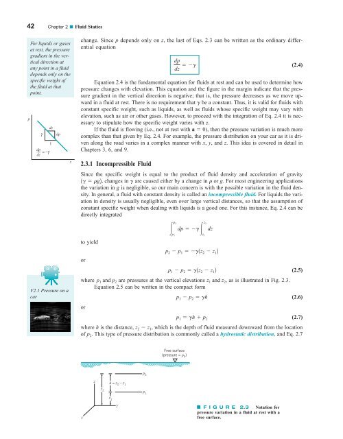
where p 1 and p 2 are pressures at the vertical elevations z 1 and z 2 , as is illustrated in Fig. 2.3.<br />
Equation 2.5 can be written in the compact form<br />
or<br />
p 2<br />
dp<br />
dz g<br />
z 2<br />
dp g<br />
p 1<br />
dz<br />
p 2 p 1 g1z 2 z 1 2<br />
p 1 p 2 gh<br />
p 1 gh p 2<br />
where h is the distance, z 2 z 1 , which is the depth of <strong>fluid</strong> measured downward from the location<br />
of p 2 . This type of pressure distribution is commonly called a hydrostatic distribution, and Eq. 2.7<br />
z 1<br />
(2.4)<br />
(2.6)<br />
(2.7)<br />
Free surface<br />
(pressure = p 0 )<br />
p 2<br />
z<br />
h = z 2 – z 1<br />
z 2<br />
p1<br />
x<br />
z 1<br />
y<br />
F I G U R E 2.3 Notation for<br />
pressure variation in a <strong>fluid</strong> at rest with a<br />
free surface.


