fluid_mechanics

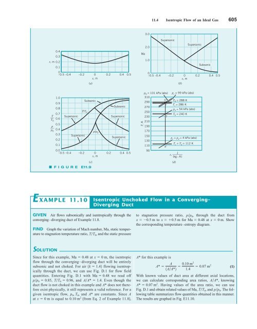
11.4 Isentropic Flow of an Ideal Gas 605
0.4
0.3
r, m 0.2
0.1
3.0
2.0
Ma
1.0
Supersonic
Supersonic
Subsonic
0
–0.5 –0.4 –0.2 0 0.2 0.4 0.5
0
–0.5 –0.4 –0.2 0 0.2 0.4 0.5
x, m x, m
(a)
(b)
T ___
T 0
p ___
p 0
p/p
p 0 = 101 kPa (abs) p c = 99 kPa (abs)
1.0
310
Subsonic
0 T
0.9
290
0 = 288 K
c T
Subsonic
c = 286 K
0.8
270
p
T/T b = 54 kPa (abs)
0 250
0.7
T
Supersonic
Supersonic
230
b b = 240 K
0.6
210
0.5
190
0.4
170
0
0.3 Supersonic
Supersonic
150
p
0.2
e = p d = 4 kPa (abs)
130
T
0.1
110
e = T d = 112 K
d
0.0
90
–0.5 –0.4 –0.2 0 0.2 0.4 0.5
J
s, _______
x, m
(kg • K)
(c)
(d)
F I G U R E E11.9
T, K
E XAMPLE 11.10
Isentropic Unchoked Flow in a Converging–
Diverging Duct
GIVEN Air flows subsonically and isentropically through the
converging–diverging duct of Example 11.8.
FIND Graph the variation of Mach number, Ma, static temperature
to stagnation temperature ratio, TT 0 , and the static pressure
to stagnation pressure ratio, pp 0 , through the duct from
x 0.5 m to x 0.5 m for Ma 0.48 at x 0 m. Show
the corresponding temperature–entropy diagram.
SOLUTION
Since for this example, Ma 0.48 at x 0 m, the isentropic
flow through the converging–diverging duct will be entirely
subsonic and not choked. For air 1k 1.42 flowing isentropically
through the duct, we can use Fig. D.1 for flow field
quantities. Entering Fig. D.1 with Ma 0.48 we read off
pp 0 0.85, TT 0 0.96, and AA* 1.4. Even though the
duct flow is not choked in this example and A* does not therefore
exist physically, it still represents a valid reference. For a
given isentropic flow, p 0 , T 0 , and A* are constants. Since A
at x 0 m is equal to 0.10 m 2 1from Eq. 2 of Example 11.82,
A* for this example is
A* A 0.10 m2
0.07 m 2
1AA*2 1.4
With known values of duct area at different axial locations,
we can calculate corresponding area ratios, AA*, knowing
A* 0.07 m 2 . Having values of the area ratio, we can use
Fig. D.1 and obtain related values of Ma, TT 0 , and pp 0 . The following
table summarizes flow quantities obtained in this manner.
The results are graphed in Fig. E11.10.
(1)