fluid_mechanics

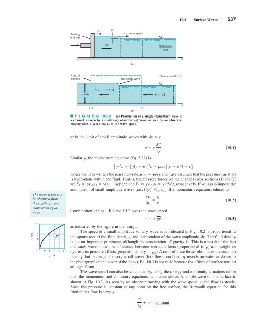
10.2 Surface Waves 537
Moving
end wall
δV
δ y
c = wave speed
δV
y
Stationary
fluid
(a)
x
Control
surface
Stationary wave
Channel width = b
y + δ y
^
V = (– c + δV)i
^
V = – c i
y
x
(1) (2)
(b)
F I G U R E 10.2 (a) Production of a single elementary wave in
a channel as seen by a stationary observer. (b) Wave as seen by an observer
moving with a speed equal to the wave speed.
c, m/s
The wave speed can
be obtained from
the continuity and
momentum equations.
10
8
6
4
c = √gy
2
0
0 2 4 6 8 10
y, m
or in the limit of small amplitude waves with dy y
Similarly, the momentum equation 1Eq. 5.222 is
c y dV
dy
1
2 gy 2 b 1 2 g1y dy2 2 b rbcy31c dV2 c4
(10.1)
where we have written the mass flowrate as m # rbcy and have assumed that the pressure variation
is hydrostatic within the fluid. That is, the pressure forces on the channel cross sections 112 and 122
are F and F 2 gy c2 A 2 gy 2 1 gy c1 A 1 g1y dy2 2 b2
b2, respectively. If we again impose the
assumption of small amplitude waves [i.e., 1dy2 2 y dy], the momentum equation reduces to
dV
dy g c
Combination of Eqs. 10.1 and 10.2 gives the wave speed
c 1gy
(10.2)
(10.3)
as indicated by the figure in the margin.
The speed of a small amplitude solitary wave as is indicated in Fig. 10.2 is proportional to
the square root of the fluid depth, y, and independent of the wave amplitude, dy. The fluid density
is not an important parameter, although the acceleration of gravity is. This is a result of the fact
that such wave motion is a balance between inertial effects 1proportional to r2 and weight or
hydrostatic pressure effects 1proportional to g rg2. A ratio of these forces eliminates the common
factor r but retains g. For very small waves (like those produced by insects on water as shown in
the photograph on the cover of the book), Eq. 10.3 is not valid because the effects of surface tension
are significant.
The wave speed can also be calculated by using the energy and continuity equations rather
than the momentum and continuity equations as is done above. A simple wave on the surface is
shown in Fig. 10.3. As seen by an observer moving with the wave speed, c, the flow is steady.
Since the pressure is constant at any point on the free surface, the Bernoulli equation for this
frictionless flow is simply
V 2
2g y constant