fluid_mechanics

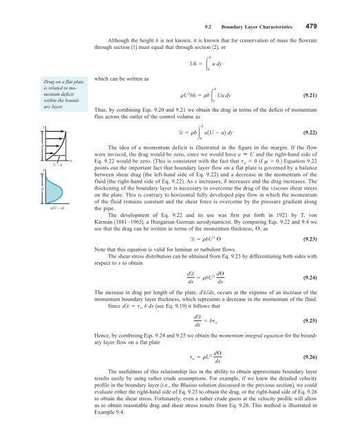
9.2 Boundary Layer Characteristics 479
Although the height h is not known, it is known that for conservation of mass the flowrate
through section 112 must equal that through section 122, or
Drag on a flat plate
is related to momentum
deficit
within the boundary
layer.
which can be written as
d
Uh u dy
d
rU 2 bh rb Uu dy
(9.21)
Thus, by combining Eqs. 9.20 and 9.21 we obtain the drag in terms of the deficit of momentum
flux across the outlet of the control volume as
0
0
y
d
d rb u1U u2 dy
0
(9.22)
δ
y
δ
U – u
u(U – u)
u
The idea of a momentum deficit is illustrated in the figure in the margin. If the flow
were inviscid, the drag would be zero, since we would have u K U and the right-hand side of
Eq. 9.22 would be zero. 1This is consistent with the fact that t w 0 if m 0.2 Equation 9.22
points out the important fact that boundary layer flow on a flat plate is governed by a balance
between shear drag 1the left-hand side of Eq. 9.222 and a decrease in the momentum of the
fluid 1the right-hand side of Eq. 9.222. As x increases, d increases and the drag increases. The
thickening of the boundary layer is necessary to overcome the drag of the viscous shear stress
on the plate. This is contrary to horizontal fully developed pipe flow in which the momentum
of the fluid remains constant and the shear force is overcome by the pressure gradient along
the pipe.
The development of Eq. 9.22 and its use was first put forth in 1921 by T. von
Kármán 11881–19632, a Hungarian/German aerodynamicist. By comparing Eqs. 9.22 and 9.4 we
see that the drag can be written in terms of the momentum thickness, , as
d rbU 2
(9.23)
Note that this equation is valid for laminar or turbulent flows.
The shear stress distribution can be obtained from Eq. 9.23 by differentiating both sides with
respect to x to obtain
dd
dx
rbU
2
d
dx
(9.24)
The increase in drag per length of the plate, dddx, occurs at the expense of an increase of the
momentum boundary layer thickness, which represents a decrease in the momentum of the fluid.
Since dd t w b dx 1see Eq. 9.192 it follows that
dd
dx bt w
(9.25)
Hence, by combining Eqs. 9.24 and 9.25 we obtain the momentum integral equation for the boundary
layer flow on a flat plate
t w rU 2 d
dx
(9.26)
The usefulness of this relationship lies in the ability to obtain approximate boundary layer
results easily by using rather crude assumptions. For example, if we knew the detailed velocity
profile in the boundary layer 1i.e., the Blasius solution discussed in the previous section2, we could
evaluate either the right-hand side of Eq. 9.23 to obtain the drag, or the right-hand side of Eq. 9.26
to obtain the shear stress. Fortunately, even a rather crude guess at the velocity profile will allow
us to obtain reasonable drag and shear stress results from Eq. 9.26. This method is illustrated in
Example 9.4.