fluid_mechanics
474 Chapter 9 ■ Flow over Immersed Bodies The boundary layer momentum thickness is defined in terms of momentum flux. Another boundary layer thickness definition, the boundary layer momentum thickness, , is often used when determining the drag on an object. Again because of the velocity deficit, U u, in the boundary layer, the momentum flux across section b–b in Fig. 9.8 is less than that across section a–a. This deficit in momentum flux for the actual boundary layer flow on a plate of width b is given by which by definition is the momentum flux in a layer of uniform speed U and thickness . That is, rbU 2 rb u1U u2 dy or ru1U u2 dA rb 0 u (9.4) 0 U a1 u U b dy All three boundary layer thickness definitions, d, d*, and , are of use in boundary layer analyses. The boundary layer concept is based on the fact that the boundary layer is thin. For the flat plate flow this means that at any location x along the plate, d x. Similarly, d* x and x. Again, this is true if we do not get too close to the leading edge of the plate 1i.e., not closer than Re x Uxn 1000 or so2. The structure and properties of the boundary layer flow depend on whether the flow is laminar or turbulent. As is illustrated in Fig. 9.9 and discussed in Sections 9.2.2 through 9.2.5, both the boundary layer thickness and the wall shear stress are different in these two regimes. 0 u1U u2 dy 9.2.2 Prandtl/Blasius Boundary Layer Solution In theory, the details of viscous, incompressible flow past any object can be obtained by solving the governing Navier–Stokes equations discussed in Section 6.8.2. For steady, two-dimensional laminar flows with negligible gravitational effects, these equations 1Eqs. 6.127a, b, and c2 reduce to the following: u 0u 0x v 0u 0y 1 0p r 0x n a 02 u 0x 02 u 2 0y b 2 u 0v 0x v 0v 0y 1 0p r 0y n a 02 v 0x 02 v 2 0y b 2 which express Newton’s second law. In addition, the conservation of mass equation, Eq. 6.31, for incompressible flow is (9.5) (9.6) 0u 0x 0v 0y 0 (9.7) δ Re x cr x τ w Laminar Turbulent x F I G U R E 9.9 Typical characteristics of boundary layer thickness and wall shear stress for laminar and turbulent boundary layers.
9.2 Boundary Layer Characteristics 475 y The Navier –Stokes equations can be simplified for boundary layer flow analysis. u → U u = v = 0 u The appropriate boundary conditions are that the fluid velocity far from the body is the upstream velocity and that the fluid sticks to the solid body surfaces. Although the mathematical problem is well-posed, no one has obtained an analytical solution to these equations for flow past any shaped body! Currently much work is being done to obtain numerical solutions to these governing equations for many flow geometries. By using boundary layer concepts introduced in the previous sections, Prandtl was able to impose certain approximations 1valid for large Reynolds number flows2, and thereby to simplify the governing equations. In 1908, H. Blasius 11883 –19702, one of Prandtl’s students, was able to solve these simplified equations for the boundary layer flow past a flat plate parallel to the flow. A brief outline of this technique and the results are presented below. Additional details may be found in the literature 1Refs. 1–32. Since the boundary layer is thin, it is expected that the component of velocity normal to the plate is much smaller than that parallel to the plate and that the rate of change of any parameter across the boundary layer should be much greater than that along the flow direction. That is, v u and 0 0x 0 0y Physically, the flow is primarily parallel to the plate and any fluid property is convected downstream much more quickly than it is diffused across the streamlines. With these assumptions it can be shown that the governing equations 1Eqs. 9.5, 9.6, and 9.72 reduce to the following boundary layer equations: 0u 0x 0v 0y 0 u 0u 0x v 0u 0y n 02 u 0y 2 Although both these boundary layer equations and the original Navier–Stokes equations are nonlinear partial differential equations, there are considerable differences between them. For one, the y momentum equation has been eliminated, leaving only the original, unaltered continuity equation and a modified x momentum equation. One of the variables, the pressure, has been eliminated, leaving only the x and y components of velocity as unknowns. For boundary layer flow over a flat plate the pressure is constant throughout the fluid. The flow represents a balance between viscous and inertial effects, with pressure playing no role. As shown by the figure in the margin, the boundary conditions for the governing boundary layer equations are that the fluid sticks to the plate u v 0 on y 0 and that outside of the boundary layer the flow is the uniform upstream flow u U. That is, u S U as y S (9.8) (9.9) (9.10) (9.11) Mathematically, the upstream velocity is approached asymptotically as one moves away from the plate. Physically, the flow velocity is within 1% of the upstream velocity at a distance of d from the plate. In mathematical terms, the Navier–Stokes equations 1Eqs. 9.5 and 9.62 and the continuity equation 1Eq. 9.72 are elliptic equations, whereas the equations for boundary layer flow 1Eqs. 9.8 and 9.92 are parabolic equations. The nature of the solutions to these two sets of equations, therefore, is different. Physically, this fact translates to the idea that what happens downstream of a given location in a boundary layer cannot affect what happens upstream of that point. That is, whether the plate shown in Fig. 9.5c ends with length / or is extended to length 2/, the flow within the first segment of length / will be the same. In addition, the presence of the plate has no effect on the flow ahead of the plate. On the other hand, ellipticity allows flow information to propagate in all directions, including upstream. In general, the solutions of nonlinear partial differential equations 1such as the boundary layer equations, Eqs. 9.8 and 9.92 are extremely difficult to obtain. However, by applying a clever coordinate transformation and change of variables, Blasius reduced the partial differential equations to an
- Page 448 and 449: 424 Chapter 8 ■ Viscous Flow in P
- Page 450 and 451: 426 Chapter 8 ■ Viscous Flow in P
- Page 452 and 453: 428 Chapter 8 ■ Viscous Flow in P
- Page 454 and 455: 430 Chapter 8 ■ Viscous Flow in P
- Page 456 and 457: 432 Chapter 8 ■ Viscous Flow in P
- Page 458 and 459: 434 Chapter 8 ■ Viscous Flow in P
- Page 460 and 461: 436 Chapter 8 ■ Viscous Flow in P
- Page 462 and 463: 438 Chapter 8 ■ Viscous Flow in P
- Page 464 and 465: 440 Chapter 8 ■ Viscous Flow in P
- Page 466 and 467: 442 Chapter 8 ■ Viscous Flow in P
- Page 468 and 469: 444 Chapter 8 ■ Viscous Flow in P
- Page 470 and 471: 446 Chapter 8 ■ Viscous Flow in P
- Page 472 and 473: 448 Chapter 8 ■ Viscous Flow in P
- Page 474 and 475: 450 Chapter 8 ■ Viscous Flow in P
- Page 476 and 477: 452 Chapter 8 ■ Viscous Flow in P
- Page 478 and 479: WARNING Stand clear of Hazard areas
- Page 480 and 481: 456 Chapter 8 ■ Viscous Flow in P
- Page 482 and 483: 458 Chapter 8 ■ Viscous Flow in P
- Page 484 and 485: 460 Chapter 8 ■ Viscous Flow in P
- Page 486 and 487: 462 Chapter 9 ■ Flow over Immerse
- Page 488 and 489: 464 Chapter 9 ■ Flow over Immerse
- Page 490 and 491: 466 Chapter 9 ■ Flow over Immerse
- Page 492 and 493: 468 Chapter 9 ■ Flow over Immerse
- Page 494 and 495: 470 Chapter 9 ■ Flow over Immerse
- Page 496 and 497: 472 Chapter 9 ■ Flow over Immerse
- Page 500 and 501: 476 Chapter 9 ■ Flow over Immerse
- Page 502 and 503: 478 Chapter 9 ■ Flow over Immerse
- Page 504 and 505: 480 Chapter 9 ■ Flow over Immerse
- Page 506 and 507: 482 Chapter 9 ■ Flow over Immerse
- Page 508 and 509: 484 Chapter 9 ■ Flow over Immerse
- Page 510 and 511: 486 Chapter 9 ■ Flow over Immerse
- Page 512 and 513: 488 Chapter 9 ■ Flow over Immerse
- Page 514 and 515: 490 Chapter 9 ■ Flow over Immerse
- Page 516 and 517: 492 Chapter 9 ■ Flow over Immerse
- Page 518 and 519: 494 Chapter 9 ■ Flow over Immerse
- Page 520 and 521: 496 Chapter 9 ■ Flow over Immerse
- Page 522 and 523: 498 Chapter 9 ■ Flow over Immerse
- Page 524 and 525: 500 Chapter 9 ■ Flow over Immerse
- Page 526 and 527: 502 Chapter 9 ■ Flow over Immerse
- Page 528 and 529: 504 Chapter 9 ■ Flow over Immerse
- Page 530 and 531: 506 Chapter 9 ■ Flow over Immerse
- Page 532 and 533: 508 Chapter 9 ■ Flow over Immerse
- Page 534 and 535: 510 Chapter 9 ■ Flow over Immerse
- Page 536 and 537: 512 Chapter 9 ■ Flow over Immerse
- Page 538 and 539: 514 Chapter 9 ■ Flow over Immerse
- Page 540 and 541: 516 Chapter 9 ■ Flow over Immerse
- Page 542 and 543: 518 Chapter 9 ■ Flow over Immerse
- Page 544 and 545: 520 Chapter 9 ■ Flow over Immerse
- Page 546 and 547: 522 Chapter 9 ■ Flow over Immerse
9.2 Boundary Layer Characteristics 475<br />
y<br />
The Navier –Stokes<br />
equations can be<br />
simplified for<br />
boundary layer flow<br />
analysis.<br />
u → U<br />
u = v = 0<br />
u<br />
The appropriate boundary conditions are that the <strong>fluid</strong> velocity far from the body is the upstream<br />
velocity and that the <strong>fluid</strong> sticks to the solid body surfaces. Although the mathematical problem is<br />
well-posed, no one has obtained an analytical solution to these equations for flow past any shaped<br />
body! Currently much work is being done to obtain numerical solutions to these governing equations<br />
for many flow geometries.<br />
By using boundary layer concepts introduced in the previous sections, Prandtl was able to<br />
impose certain approximations 1valid for large Reynolds number flows2, and thereby to simplify<br />
the governing equations. In 1908, H. Blasius 11883 –19702, one of Prandtl’s students, was able to<br />
solve these simplified equations for the boundary layer flow past a flat plate parallel to the flow.<br />
A brief outline of this technique and the results are presented below. Additional details may be<br />
found in the literature 1Refs. 1–32.<br />
Since the boundary layer is thin, it is expected that the component of velocity normal to the<br />
plate is much smaller than that parallel to the plate and that the rate of change of any parameter<br />
across the boundary layer should be much greater than that along the flow direction. That is,<br />
v u and 0<br />
0x 0<br />
0y<br />
Physically, the flow is primarily parallel to the plate and any <strong>fluid</strong> property is convected downstream<br />
much more quickly than it is diffused across the streamlines.<br />
With these assumptions it can be shown that the governing equations 1Eqs. 9.5, 9.6, and 9.72<br />
reduce to the following boundary layer equations:<br />
0u<br />
0x 0v<br />
0y 0<br />
u 0u<br />
0x v 0u<br />
0y n 02 u<br />
0y 2<br />
Although both these boundary layer equations and the original Navier–Stokes equations are nonlinear<br />
partial differential equations, there are considerable differences between them. For one, the<br />
y momentum equation has been eliminated, leaving only the original, unaltered continuity equation<br />
and a modified x momentum equation. One of the variables, the pressure, has been eliminated,<br />
leaving only the x and y components of velocity as unknowns. For boundary layer flow over a flat<br />
plate the pressure is constant throughout the <strong>fluid</strong>. The flow represents a balance between viscous<br />
and inertial effects, with pressure playing no role.<br />
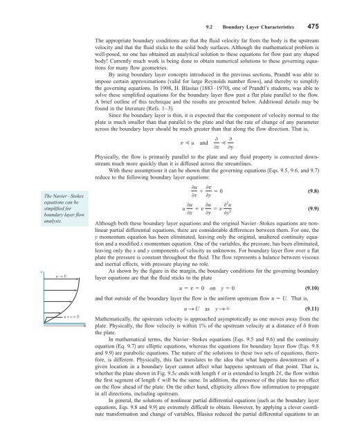
As shown by the figure in the margin, the boundary conditions for the governing boundary<br />
layer equations are that the <strong>fluid</strong> sticks to the plate<br />
u v 0 on y 0<br />
and that outside of the boundary layer the flow is the uniform upstream flow u U. That is,<br />
u S U as y S <br />
(9.8)<br />
(9.9)<br />
(9.10)<br />
(9.11)<br />
Mathematically, the upstream velocity is approached asymptotically as one moves away from the<br />
plate. Physically, the flow velocity is within 1% of the upstream velocity at a distance of d from<br />
the plate.<br />
In mathematical terms, the Navier–Stokes equations 1Eqs. 9.5 and 9.62 and the continuity<br />
equation 1Eq. 9.72 are elliptic equations, whereas the equations for boundary layer flow 1Eqs. 9.8<br />
and 9.92 are parabolic equations. The nature of the solutions to these two sets of equations, therefore,<br />
is different. Physically, this fact translates to the idea that what happens downstream of a<br />
given location in a boundary layer cannot affect what happens upstream of that point. That is,<br />
whether the plate shown in Fig. 9.5c ends with length / or is extended to length 2/, the flow within<br />
the first segment of length / will be the same. In addition, the presence of the plate has no effect<br />
on the flow ahead of the plate. On the other hand, ellipticity allows flow information to propagate<br />
in all directions, including upstream.<br />
In general, the solutions of nonlinear partial differential equations 1such as the boundary layer<br />
equations, Eqs. 9.8 and 9.92 are extremely difficult to obtain. However, by applying a clever coordinate<br />
transformation and change of variables, Blasius reduced the partial differential equations to an


