fluid_mechanics

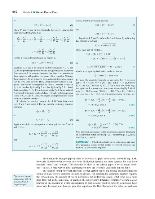
440 Chapter 8 ■ Viscous Flow in Pipes
or
322 V 2 1 0.4V 2 3
(2)
where V 1 and V 3 are in fts. Similarly the energy equation for
fluid flowing from B and C is
or
For the given conditions this can be written as
Equations 1, 2, and 3 1in terms of the three unknowns V 1 , V 2 , and
V 3 2 are the governing equations for this flow, provided the fluid flows
from reservoir B. It turns out, however, that there is no solution for
these equations with positive, real values of the velocities. Although
these equations do not appear to be complicated, there is no simple
way to solve them directly. Thus, a trial-and-error solution is suggested.
This can be accomplished as follows. Assume a value of
V 1 7 0, calculate V 3 from Eq. 2, and then V 2 from Eq. 3. It is found
that the resulting V 1 , V 2 , V 3 trio does not satisfy Eq. 1 for any value of
V 1 assumed. There is no solution to Eqs. 1, 2, and 3 with real, positive
values of V 1 , V 2 , and V 3 . Thus, our original assumption of flow out of
reservoir B must be incorrect.
To obtain the solution, assume the fluid flows into reservoirs
B and C and out of A. For this case the continuity equation
becomes
or
Application of the energy equation between points A and B and A
and C gives
and
p B
g V 2 B
2g z B p C
g V 2 C
2g z C f / 2 V 2 2
2
D 2 2g f / 3 V 2 3
3
D 3 2g
z B f / 2 V 2 2
2
D 2 2g f / 3 V 2 3
3
D 3 2g
64.4 0.5V 2 2 0.4V 2 3
Q 1 Q 2 Q 3
V 1 V 2 V 3
z A z B f / 1 V 2 1
1
D 1 2g f / 2 V 2 2
2
D 2 2g
z A z C f / 1 V 2 1
1
D 1 2g f / 2
3 V 3
3
D 3 2g
(3)
(4)
which, with the given data, become
and
Equations 4, 5, and 6 can be solved as follows. By subtracting
Eq. 5 from 6 we obtain
Thus, Eq. 5 can be written as
or
which, upon squaring both sides, can be written as
By using the quadratic formula we can solve for V 2 to obtain
either V 2 2 452 or V 2 2
2 8.30. Thus, either V 2 21.3 fts or
V 2 2.88 fts. The value V 2 21.3 fts is not a root of the original
equations. It is an extra root introduced by squaring Eq. 7, which
with V 2 21.3 becomes “1140 1140.” Thus, V 2 2.88 fts
and from Eq. 5, V 1 15.9 fts. The corresponding flowrates are
and
258 V 2 1 0.5 V 2 2
322 V 2 1 0.4 V 2 3
V 3 2160 1.25V 2 2
258 1V 2 V 3 2 2 0.5V 2 2
1V 2 2160 1.25V 2 22 2 0.5V 2 2
2V 2 2160 1.25V 2 2 98 2.75V 2 2
V 4 2 460 V 2 2 3748 0
Q 1 A 1 V 1 p 4 D2 1V 1 p 4 11 ft22 115.9 fts2
12.5 ft 3 s from A
Q 2 A 2 V 2 p 4 D2 2V 2 p 4 11 ft22 12.88 fts2
2.26 ft 3 s into B
Q 3 Q 1 Q 2 112.5 2.262 ft 3 s
10.2 ft 3 s into C
(5)
(6)
(7)
(Ans)
(Ans)
(Ans)
Note the slight differences in the governing equations depending
on the direction of the flow in pipe 122—compare Eqs. 1, 2, and 3
with Eqs. 4, 5, and 6.
COMMENT If the friction factors were not given, a trial-anderror
procedure similar to that needed for Type II problems 1see
Section 8.5.12 would be required.
Pipe network problems
can be solved
using node and
loop concepts.
The ultimate in multiple pipe systems is a network of pipes such as that shown in Fig. 8.38.
Networks like these often occur in city water distribution systems and other systems that may have
multiple “inlets” and “outlets.” The direction of flow in the various pipes is by no means obvious—in
fact, it may vary in time, depending on how the system is used from time to time.
The solution for pipe network problems is often carried out by use of node and loop equations
similar in many ways to that done in electrical circuits. For example, the continuity equation requires
that for each node 1the junction of two or more pipes2 the net flowrate is zero. What flows into a node
must flow out at the same rate. In addition, the net pressure difference completely around a loop
1starting at one location in a pipe and returning to that location2 must be zero. By combining these
ideas with the usual head loss and pipe flow equations, the flow throughout the entire network can