fluid_mechanics

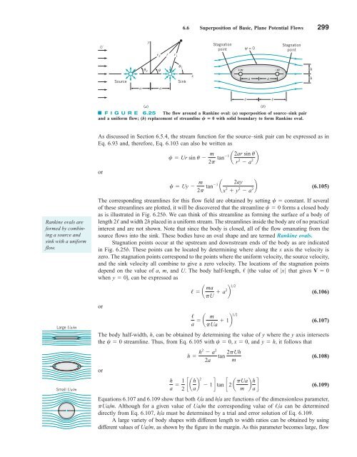
6.6 Superposition of Basic, Plane Potential Flows 299
U
y
Stagnation
point
ψ = 0
Stagnation
point
r 2
r r 1
Source
a
θ2
θ
a
θ 1
Sink
x
+m –m
a
a
h
h
(a)
(b)
F I G U R E 6.25 The flow around a Rankine oval: (a) superposition of source–sink pair
and a uniform flow; (b) replacement of streamline C 0 with solid boundary to form Rankine oval.
Rankine ovals are
formed by combining
a source and
sink with a uniform
flow.
Large Ua/m
Small Ua/m
As discussed in Section 6.5.4, the stream function for the source–sink pair can be expressed as in
Eq. 6.93 and, therefore, Eq. 6.103 can also be written as
or
(6.105)
The corresponding streamlines for this flow field are obtained by setting c constant. If several
of these streamlines are plotted, it will be discovered that the streamline c 0 forms a closed body
as is illustrated in Fig. 6.25b. We can think of this streamline as forming the surface of a body of
length 2/ and width 2h placed in a uniform stream. The streamlines inside the body are of no practical
interest and are not shown. Note that since the body is closed, all of the flow emanating from the
source flows into the sink. These bodies have an oval shape and are termed Rankine ovals.
Stagnation points occur at the upstream and downstream ends of the body as are indicated
in Fig. 6.25b. These points can be located by determining where along the x axis the velocity is
zero. The stagnation points correspond to the points where the uniform velocity, the source velocity,
and the sink velocity all combine to give a zero velocity. The locations of the stagnation points
depend on the value of a, m, and U. The body half-length, / 1the value of 0x 0 that gives V 0
when y 02, can be expressed as
or
(6.106)
(6.107)
The body half-width, h, can be obtained by determining the value of y where the y axis intersects
the c 0 streamline. Thus, from Eq. 6.105 with c 0, x 0, and y h, it follows that
or
c Ur sin u m 2p tan1 a
c Uy m 2ay
2p tan1 a
x 2 y 2 a 2b
/ a ma 12
pU a2 b
/
a a m 12
pUa 1b
h h2 a 2
tan 2pUh
2a m
2ar sin u
r
2 a b 2
h
a 1 2 cah a b 2
1 d tan c 2 a pUa
m b h
a d
(6.108)
(6.109)
Equations 6.107 and 6.109 show that both /a and ha are functions of the dimensionless parameter,
pUam. Although for a given value of Uam the corresponding value of /a can be determined
directly from Eq. 6.107, ha must be determined by a trial and error solution of Eq. 6.109.
A large variety of body shapes with different length to width ratios can be obtained by using
different values of Uam, as shown by the figure in the margin. As this parameter becomes large, flow