fluid_mechanics
294 Chapter 6 ■ Differential Analysis of Fluid Flow which can be rewritten as tan a 2pc m b tan1u 1 u 2 2 tan u 1 tan u 2 1 tan u 1 tan u 2 (6.92) From Fig. 6.22 it follows that y Source Sink A doublet is formed by letting a source and sink approach one another. x and These results substituted into Eq. 6.92 give so that tan u 1 tan u 2 tan a 2pc m r sin u r cos u a r sin u r cos u a b 2ar sin u r 2 a 2 c m 2ar sin u 2p tan1 a r 2 a b 2 (6.93) The figure in the margin shows typical streamlines for this flow. For small values of the distance a c m 2ar sin u sin u mar 2p r 2 2 a p1r 2 a 2 2 (6.94) since the tangent of an angle approaches the value of the angle for small angles. The so-called doublet is formed by letting the source and sink approach one another 1a S 02 while increasing the strength m 1m S 2 so that the product map remains constant. In this case, since r1r 2 a 2 2 S 1r, Eq. 6.94 reduces to c K sin u r (6.95) where K, a constant equal to map, is called the strength of the doublet. The corresponding velocity potential for the doublet is f K cos u r (6.96) Plots of lines of constant c reveal that the streamlines for a doublet are circles through the origin tangent to the x axis as shown in Fig. 6.23. Just as sources and sinks are not physically realistic entities, neither are doublets. However, the doublet when combined with other basic potential flows y x F I G U R E 6.23 doublet. Streamlines for a
TABLE 6.1 Summary of Basic, Plane Potential Flows 6.6 Superposition of Basic, Plane Potential Flows 295 Description of Velocity Flow Field Velocity Potential Stream Function Components a Uniform flow at angle a with the x axis 1see Fig. 6.16b2 f U1x cos a y sin a2 c U1 y cos a x sin a2 u U cos a v U sin a Source or sink 1see Fig. 6.172 m 7 0 source m 6 0 sink Free vortex 1see Fig. 6.182 7 0 counterclockwise motion 6 0 clockwise motion Doublet 1see Fig. 6.232 f m c m v r m 2p ln r 2p u 2pr f 2p u c 2p ln r v r 0 v u 0 f K cos u r c K sin u r v u 2pr v r K cos u r 2 v u K sin u r 2 a Velocity components are related to the velocity potential and stream function through the relationships: u 0f . 0x 0c v 0f 0y 0y 0c v 0x r 0f 0r 1 0c v r 0u u 1 0f r 0u 0c 0r provides a useful representation of some flow fields of practical interest. For example, we will determine in Section 6.6.3 that the combination of a uniform flow and a doublet can be used to represent the flow around a circular cylinder. Table 6.1 provides a summary of the pertinent equations for the basic, plane potential flows considered in the preceding sections. 6.6 Superposition of Basic, Plane Potential Flows As was discussed in the previous section, potential flows are governed by Laplace’s equation, which is a linear partial differential equation. It therefore follows that the various basic velocity potentials and stream functions can be combined to form new potentials and stream functions. 1Why is this true?2 Whether such combinations yield useful results remains to be seen. It is to be noted that any streamline in an inviscid flow field can be considered as a solid boundary, since the conditions along a solid boundary and a streamline are the same—that is, there is no flow through the boundary or the streamline. Thus, if we can combine some of the basic velocity potentials or stream functions to yield a streamline that corresponds to a particular body shape of interest, that combination can be used to describe in detail the flow around that body. This method of solving some interesting flow problems, commonly called the method of superposition, is illustrated in the following three sections. Flow around a half-body is obtained by the addition of a source to a uniform flow. 6.6.1 Source in a Uniform Stream—Half-Body Consider the superposition of a source and a uniform flow as shown in Fig. 6.24a. The resulting stream function is c c uniform flow c source Ur sin u m 2p u (6.97)
- Page 268 and 269: 244 Chapter 5 ■ Finite Control Vo
- Page 270 and 271: 246 Chapter 5 ■ Finite Control Vo
- Page 272 and 273: 248 Chapter 5 ■ Finite Control Vo
- Page 274 and 275: 250 Chapter 5 ■ Finite Control Vo
- Page 276 and 277: 252 Chapter 5 ■ Finite Control Vo
- Page 278 and 279: 254 Chapter 5 ■ Finite Control Vo
- Page 280 and 281: 256 Chapter 5 ■ Finite Control Vo
- Page 282 and 283: 258 Chapter 5 ■ Finite Control Vo
- Page 284 and 285: 260 Chapter 5 ■ Finite Control Vo
- Page 286 and 287: 262 Chapter 5 ■ Finite Control Vo
- Page 288 and 289: 264 Chapter 6 ■ Differential Anal
- Page 290 and 291: ) 266 Chapter 6 ■ Differential An
- Page 292 and 293: 268 Chapter 6 ■ Differential Anal
- Page 294 and 295: 270 Chapter 6 ■ Differential Anal
- Page 296 and 297: 272 Chapter 6 ■ Differential Anal
- Page 298 and 299: 274 Chapter 6 ■ Differential Anal
- Page 300 and 301: 276 Chapter 6 ■ Differential Anal
- Page 302 and 303: 278 Chapter 6 ■ Differential Anal
- Page 304 and 305: 280 Chapter 6 ■ Differential Anal
- Page 306 and 307: 282 Chapter 6 ■ Differential Anal
- Page 308 and 309: 284 Chapter 6 ■ Differential Anal
- Page 310 and 311: 286 Chapter 6 ■ Differential Anal
- Page 312 and 313: 288 Chapter 6 ■ Differential Anal
- Page 314 and 315: 290 Chapter 6 ■ Differential Anal
- Page 316 and 317: 292 Chapter 6 ■ Differential Anal
- Page 320 and 321: 296 Chapter 6 ■ Differential Anal
- Page 322 and 323: 298 Chapter 6 ■ Differential Anal
- Page 324 and 325: 300 Chapter 6 ■ Differential Anal
- Page 326 and 327: 302 Chapter 6 ■ Differential Anal
- Page 328 and 329: 304 Chapter 6 ■ Differential Anal
- Page 330 and 331: 306 Chapter 6 ■ Differential Anal
- Page 332 and 333: 308 Chapter 6 ■ Differential Anal
- Page 334 and 335: 310 Chapter 6 ■ Differential Anal
- Page 336 and 337: 312 Chapter 6 ■ Differential Anal
- Page 338 and 339: 314 Chapter 6 ■ Differential Anal
- Page 340 and 341: 316 Chapter 6 ■ Differential Anal
- Page 342 and 343: 318 Chapter 6 ■ Differential Anal
- Page 344 and 345: 320 Chapter 6 ■ Differential Anal
- Page 346 and 347: 322 Chapter 6 ■ Differential Anal
- Page 348 and 349: 324 Chapter 6 ■ Differential Anal
- Page 350 and 351: 326 Chapter 6 ■ Differential Anal
- Page 352 and 353: 328 Chapter 6 ■ Differential Anal
- Page 354 and 355: 330 Chapter 6 ■ Differential Anal
- Page 356 and 357: 7 Dimensional Analysis, Similitude,
- Page 358 and 359: 334 Chapter 7 ■ Dimensional Analy
- Page 360 and 361: 336 Chapter 7 ■ Dimensional Analy
- Page 362 and 363: 338 Chapter 7 ■ Dimensional Analy
- Page 364 and 365: 340 Chapter 7 ■ Dimensional Analy
- Page 366 and 367: 342 Chapter 7 ■ Dimensional Analy
294 Chapter 6 ■ Differential Analysis of Fluid Flow<br />
which can be rewritten as<br />
tan a 2pc<br />
m b tan1u 1 u 2 2 tan u 1 tan u 2<br />
1 tan u 1 tan u 2<br />
(6.92)<br />
From Fig. 6.22 it follows that<br />
y<br />
Source<br />
Sink<br />
A doublet is formed<br />
by letting a source<br />
and sink approach<br />
one another.<br />
x<br />
and<br />
These results substituted into Eq. 6.92 give<br />
so that<br />
tan u 1 <br />
tan u 2 <br />
tan a 2pc<br />
m<br />
r sin u<br />
r cos u a<br />
r sin u<br />
r cos u a<br />
b 2ar sin u<br />
r<br />
2 a 2<br />
c m 2ar sin u<br />
2p tan1 a<br />
r 2 a b 2<br />
(6.93)<br />
The figure in the margin shows typical streamlines for this flow. For small values of the distance a<br />
c m 2ar sin u sin u<br />
mar<br />
2p r<br />
2 2<br />
a p1r 2 a 2 2<br />
(6.94)<br />
since the tangent of an angle approaches the value of the angle for small angles.<br />
The so-called doublet is formed by letting the source and sink approach one another 1a S 02<br />
while increasing the strength m 1m S 2 so that the product map remains constant. In this case,<br />
since r1r 2 a 2 2 S 1r, Eq. 6.94 reduces to<br />
c K sin u<br />
r<br />
(6.95)<br />
where K, a constant equal to map, is called the strength of the doublet. The corresponding velocity<br />
potential for the doublet is<br />
f K cos u<br />
r<br />
(6.96)<br />
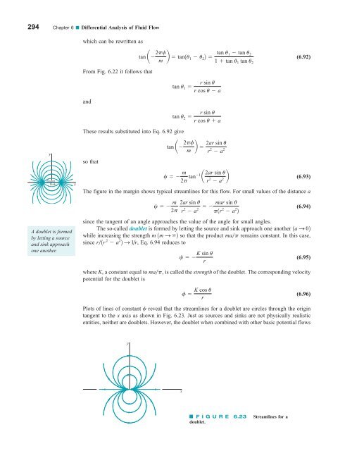
Plots of lines of constant c reveal that the streamlines for a doublet are circles through the origin<br />
tangent to the x axis as shown in Fig. 6.23. Just as sources and sinks are not physically realistic<br />
entities, neither are doublets. However, the doublet when combined with other basic potential flows<br />
y<br />
x<br />
F I G U R E 6.23<br />
doublet.<br />
Streamlines for a


