fluid_mechanics

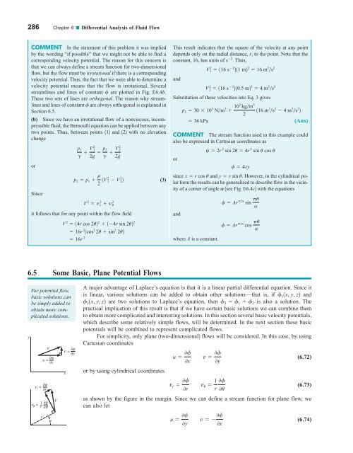
286 Chapter 6 ■ Differential Analysis of Fluid Flow
COMMENT In the statement of this problem it was implied
by the wording “if possible” that we might not be able to find a
corresponding velocity potential. The reason for this concern is
that we can always define a stream function for two-dimensional
flow, but the flow must be irrotational if there is a corresponding
velocity potential. Thus, the fact that we were able to determine a
velocity potential means that the flow is irrotational. Several
streamlines and lines of constant f are plotted in Fig. E6.4b.
These two sets of lines are orthogonal. The reason why streamlines
and lines of constant f are always orthogonal is explained in
Section 6.5.
(b) Since we have an irrotational flow of a nonviscous, incompressible
fluid, the Bernoulli equation can be applied between any
two points. Thus, between points 112 and 122 with no elevation
change
or
Since
p 1
g V 2 1
2g p 2
g V 2 2
2g
p 2 p 1 r 2 1V 2 1 V 2 22
V 2 v 2 r v 2 u
it follows that for any point within the flow field
V 2 14r cos 2u2 2 14r sin 2u2 2
16r 2 1cos 2 2u sin 2 2u2
16r 2
(3)
This result indicates that the square of the velocity at any point
depends only on the radial distance, r, to the point. Note that the
constant, 16, has units of s 2 . Thus,
and
Substitution of these velocities into Eq. 3 gives
COMMENT The stream function used in this example could
also be expressed in Cartesian coordinates as
or
since x r cos u and y r sin u. However, in the cylindrical polar
form the results can be generalized to describe flow in the vicinity
of a corner of angle a 1see Fig. E6.4c2 with the equations
and
p 2 30 10 3 Nm 2 103 kgm 3
116 m 2 s 2 4 m 2 s 2 2
2
36 kPa
(Ans)
where A is a constant.
V 2 1 116 s 2 211 m2 2 16 m 2 s 2
V 2 2 116 s 2 210.5 m2 2 4 m 2 s 2
c 2r 2 sin 2u 4r 2 sin u cos u
c 4xy
c Ar p a
sin pu
a
f Ar p a
cos pu
a
6.5 Some Basic, Plane Potential Flows
y
For potential flow,
basic solutions can
be simply added to
obtain more complicated
solutions.
V
∂φ
u =
∂ x
∂φ
v r =
∂r
∂φ
v θ =
1__ r ∂θ
r
θ
V
∂φ
v =
∂ y
x
A major advantage of Laplace’s equation is that it is a linear partial differential equation. Since it
is linear, various solutions can be added to obtain other solutions—that is, if f 1 1x, y, z2 and
f 2 1x, y, z2 are two solutions to Laplace’s equation, then f 3 f 1 f 2 is also a solution. The
practical implication of this result is that if we have certain basic solutions we can combine them
to obtain more complicated and interesting solutions. In this section several basic velocity potentials,
which describe some relatively simple flows, will be determined. In the next section these basic
potentials will be combined to represent complicated flows.
For simplicity, only plane 1two-dimensional2 flows will be considered. In this case, by using
Cartesian coordinates
or by using cylindrical coordinates
u 0f
0x
v r 0f
0r
(6.72)
(6.73)
as shown by the figure in the margin. Since we can define a stream function for plane flow, we
can also let
u 0c
0y
v 0f
0y
v u 1 0f
r 0u
v 0c
0x
(6.74)