fluid_mechanics

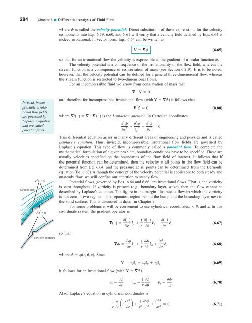
284 Chapter 6 ■ Differential Analysis of Fluid Flow
where f is called the velocity potential. Direct substitution of these expressions for the velocity
components into Eqs. 6.59, 6.60, and 6.61 will verify that a velocity field defined by Eqs. 6.64 is
indeed irrotational. In vector form, Eqs. 6.64 can be written as
V f
(6.65)
Inviscid, incompressible,
irrotational
flow fields
are governed by
Laplace’s equation
and are called
potential flows.
Streamlines
2 0
2 0
Vorticity contours
so that for an irrotational flow the velocity is expressible as the gradient of a scalar function f.
The velocity potential is a consequence of the irrotationality of the flow field, whereas the
stream function is a consequence of conservation of mass (see Section 6.2.3). It is to be noted,
however, that the velocity potential can be defined for a general three-dimensional flow, whereas
the stream function is restricted to two-dimensional flows.
For an incompressible fluid we know from conservation of mass that
and therefore for incompressible, irrotational flow 1with V f2 it follows that
where 2 1 2 1 2 is the Laplacian operator. In Cartesian coordinates
(6.66)
This differential equation arises in many different areas of engineering and physics and is called
Laplace’s equation. Thus, inviscid, incompressible, irrotational flow fields are governed by
Laplace’s equation. This type of flow is commonly called a potential flow. To complete the
mathematical formulation of a given problem, boundary conditions have to be specified. These are
usually velocities specified on the boundaries of the flow field of interest. It follows that if
the potential function can be determined, then the velocity at all points in the flow field can be
determined from Eq. 6.64, and the pressure at all points can be determined from the Bernoulli
equation 1Eq. 6.632. Although the concept of the velocity potential is applicable to both steady and
unsteady flow, we will confine our attention to steady flow.
Potential flows, governed by Eqs. 6.64 and 6.66, are irrotational flows. That is, the vorticity
is zero throughout. If vorticity is present (e.g., boundary layer, wake), then the flow cannot be
described by Laplace’s equation. The figure in the margin illustrates a flow in which the vorticity
is not zero in two regions—the separated region behind the bump and the boundary layer next to
the solid surface. This is discussed in detail in Chapter 9.
For some problems it will be convenient to use cylindrical coordinates, r, u, and z. In this
coordinate system the gradient operator is
so that
where f f1r, u, z2. Since
V 0
2 f 0
0 2 f
0x 2 02 f
0y 2 02 f
0z 2 0
1 2 01 2
0r ê r 1 r
f 0f
0r ê r 1 r
V v r ê r v u ê u v z ê z
it follows for an irrotational flow 1with V f2
01 2
0u ê u 01 2
0z ê z
0f
0u ê u 0f
0z ê z
(6.67)
(6.68)
(6.69)
v r 0f
0r
v u 1 0f
r 0u
v z 0f
0z
(6.70)
Also, Laplace’s equation in cylindrical coordinates is
1
r
0 0f
ar
0r 0r b 1 02 f
r 2 0u 02 f
2 0z 0 2
(6.71)