fluid_mechanics

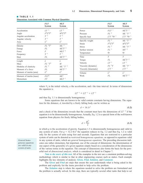
1.2 Dimensions, Dimensional Homogeneity, and Units 5
TABLE 1.1
Dimensions Associated with Common Physical Quantities
FLT
System
MLT
System
FLT
System
MLT
System
Acceleration
Angle
Angular acceleration
Angular velocity
Area
Density
Energy
Force
Frequency
Heat
2
LT
F 0 L 0 T
T
2
1
T
L 2
FL 4 2
T
FL
F
1
T
FL
M 0 L 0 T
T
2
1
T
L 2
ML 3
ML 2 2
T
2
MLT
1
T
ML 2 2
T
Length L L
Mass
FL 1 2
T M
Modulus of elasticity
Moment of a force
FL 2
FL
ML 1 T
ML 2 2
T
Moment of inertia 1area2 L 4
L 4
Moment of inertia 1mass2 FLT 2 ML 2
Momentum FT MLT 1
0
2
LT
0
2
Power
Pressure
Specific heat
Specific weight
Strain
Stress
Surface tension
Temperature
Time T T
Torque
FL
ML 2 2
T
Velocity
Viscosity 1dynamic2
Viscosity 1kinematic2
1
FLT
FL 2
L 2 T
2 1
FL 3
F 0 L 0 0
T
FL 2
FL 1
1
LT
FL 2 T
L 2 1
T
Volume
Work FL ML 2 T 2
L 3
ML 2 3
T
ML 1 2
T
L 2 T
2 1
ML 2 2
T
M
0 L 0 0
T
ML 1 2
T
2
MT
1
LT
ML 1 1
T
L 2 1
T
L 3
General homogeneous
equations
are valid in any
system of units.
where V 0 is the initial velocity, a the acceleration, and t the time interval. In terms of dimensions
the equation is
LT 1 LT 1 LT 1
and thus Eq. 1.1 is dimensionally homogeneous.
Some equations that are known to be valid contain constants having dimensions. The equation
for the distance, d, traveled by a freely falling body can be written as
d 16.1t 2
and a check of the dimensions reveals that the constant must have the dimensions of LT 2 if the
equation is to be dimensionally homogeneous. Actually, Eq. 1.2 is a special form of the well-known
equation from physics for freely falling bodies,
d gt 2
(1.3)
2
in which g is the acceleration of gravity. Equation 1.3 is dimensionally homogeneous and valid in
any system of units. For g 32.2 fts 2 the equation reduces to Eq. 1.2 and thus Eq. 1.2 is valid
only for the system of units using feet and seconds. Equations that are restricted to a particular
system of units can be denoted as restricted homogeneous equations, as opposed to equations valid
in any system of units, which are general homogeneous equations. The preceding discussion indicates
one rather elementary, but important, use of the concept of dimensions: the determination of
one aspect of the generality of a given equation simply based on a consideration of the dimensions
of the various terms in the equation. The concept of dimensions also forms the basis for the powerful
tool of dimensional analysis, which is considered in detail in Chapter 7.
Note to the users of this text. All of the examples in the text use a consistent problem-solving
methodology which is similar to that in other engineering courses such as statics. Each example
highlights the key elements of analysis: Given, Find, Solution, and Comment.
The Given and Find are steps that ensure the user understands what is being asked in the
problem and explicitly list the items provided to help solve the problem.
The Solution step is where the equations needed to solve the problem are formulated and
the problem is actually solved. In this step, there are typically several other tasks that help to set
(1.2)