fluid_mechanics

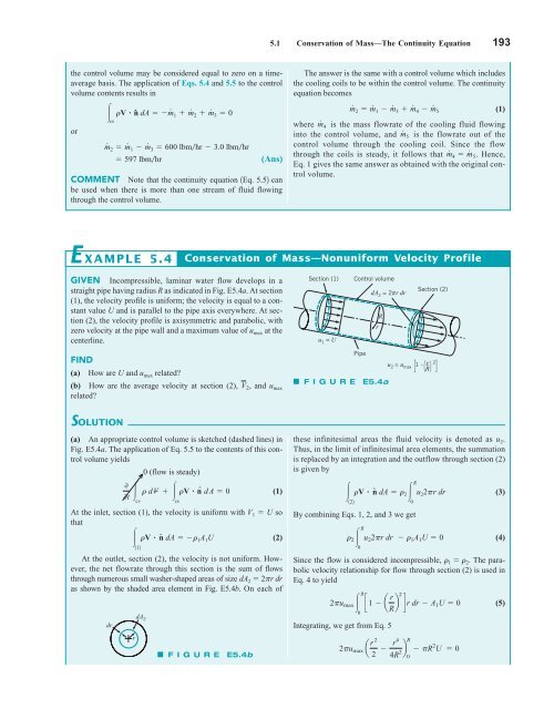
5.1 Conservation of Mass—The Continuity Equation 193
the control volume may be considered equal to zero on a timeaverage
basis. The application of Eqs. 5.4 and 5.5 to the control
volume contents results in
rV nˆ dA m # 1 m # 2 m # 3 0
cs
or
m # 2 m # 1 m # 3 600 lbmhr 3.0 lbmhr
597 lbmhr
(Ans)
COMMENT Note that the continuity equation 1Eq. 5.52 can
be used when there is more than one stream of fluid flowing
through the control volume.
The answer is the same with a control volume which includes
the cooling coils to be within the control volume. The continuity
equation becomes
m # 2 m # 1 m # 3 m # 4 m # 5
where m # 4 is the mass flowrate of the cooling fluid flowing
into the control volume, and m # 5 is the flowrate out of the
control volume through the cooling coil. Since the flow
through the coils is steady, it follows that m # 4 m # 5. Hence,
Eq. 1 gives the same answer as obtained with the original control
volume.
(1)
E XAMPLE 5.4
Conservation of Mass—Nonuniform Velocity Profile
GIVEN Incompressible, laminar water flow develops in a
straight pipe having radius R as indicated in Fig. E5.4a. At section
(1), the velocity profile is uniform; the velocity is equal to a constant
value U and is parallel to the pipe axis everywhere. At section
(2), the velocity profile is axisymmetric and parabolic, with
zero velocity at the pipe wall and a maximum value of u max at the
centerline.
FIND
(a) How are U and u max related?
(b) How are the average velocity at section (2), V 2 , and u max
related?
Section (1)
u 1 = U
Control volume
Pipe
dA 2 = 2 πr dr
R
r
F I G U R E E5.4a
Section (2)
[ ( ) ]
u 2 = u max 1 - _ r 2
R
SOLUTION
these infinitesimal areas the fluid velocity is denoted as u .
(a) An appropriate control volume is sketched (dashed lines) in
2u max R
c 1 a r 2
(5)
R b d r dr A 1 U 0
0
dA 2
Fig. E5.4a. The application of Eq. 5.5 to the contents of this control
volume yields
0 (flow is steady)
2
Thus, in the limit of infinitesimal area elements, the summation
is replaced by an integration and the outflow through section (2)
is given by
0
r dV (1)
0t
cv
rV nˆ dA 0
rV ˆn dA r 2 R
u 2 2pr dr
cs
122
0
(3)
At the inlet, section (1), the velocity is uniform with V 1 U so
that
By combining Eqs. 1, 2, and 3 we get
112rV ˆn dA r 1 A 1 U
(2)
2 R
u 2 2r dr 1 A 1 U 0
0
(4)
At the outlet, section (2), the velocity is not uniform. However,
the net flowrate through this section is the sum of flows
through numerous small washer-shaped areas of size dA 2 2r dr
Since the flow is considered incompressible, 1 2 . The parabolic
velocity relationship for flow through section (2) is used in
Eq. 4 to yield
as shown by the shaded area element in Fig. E5.4b. On each of
dr
Integrating, we get from Eq. 5
r
F I G U R E E5.4b
2u max a r 2
2 r4 R
4R 2b R 2 U 0
0