fluid_mechanics

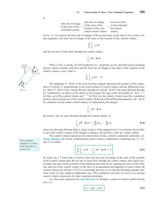
V
Control
surface
^
n
^
Vn < 0
V
^
n
^
Vn > 0
or
time rate of change
of the mass of the
coincident system
In Eq. 5.3, we express the time rate of change of the system mass as the sum of two control volume
quantities, the time rate of change of the mass of the contents of the control volume,
and the net rate of mass flow through the control surface,
5.1 Conservation of Mass—The Continuity Equation 189
time rate of change net rate of flow
of the mass of the of mass through
contents of the coincident
control volume
the control
surface
0
0t cv
r dV
cs
rV nˆ dA
When a flow is steady, all field properties 1i.e., properties at any specified point2 including
density remain constant with time and the time rate of change of the mass of the contents of the
control volume is zero. That is,
0
0t r dV0
cv
The integrand, V nˆ dA, in the mass flowrate integral represents the product of the component
of velocity, V, perpendicular to the small portion of control surface and the differential area,
dA. Thus, V nˆ dA is the volume flowrate through dA and rV nˆ dA is the mass flowrate through
dA. Furthermore, as shown in the sketch in the margin, the sign of the dot product V nˆ is “”
for flow out of the control volume and “” for flow into the control volume since nˆ is considered
positive when it points out of the control volume. When all of the differential quantities, rV nˆ dA,
are summed over the entire control surface, as indicated by the integral
cs
rV nˆ dA
the result is the net mass flowrate through the control surface, or
The continuity
equation is a statement
that mass is
conserved.
cs
rV nˆ dA a m # out a m # in
where m # is the mass flowrate 1lbms, slugs or kgs2. If the integral in Eq. 5.4 is positive, the net flow
is out of the control volume; if the integral is negative, the net flow is into the control volume.
The control volume expression for conservation of mass, which is commonly called the continuity
equation, for a fixed, nondeforming control volume is obtained by combining Eqs. 5.1, 5.2,
and 5.3 to obtain
0
0t cv
r dV cs
rV nˆ dA 0
(5.4)
(5.5)
In words, Eq. 5.5 states that to conserve mass the time rate of change of the mass of the contents
of the control volume plus the net rate of mass flow through the control surface must equal zero.
Actually, the same result could have been obtained more directly by equating the rates of mass flow
into and out of the control volume to the rates of accumulation and depletion of mass within the
control volume 1see Section 3.6.22. It is reassuring, however, to see that the Reynolds transport theorem
works for this simple-to-understand case. This confidence will serve us well as we develop
control volume expressions for other important principles.
An often-used expression for mass flowrate, m # , through a section of control surface having
area A is
m # rQ rAV
(5.6)