fluid_mechanics
186 Chapter 4 ■ Fluid Kinematics Cylinder Plunger V p = 0.03 m/s V = 5 m/s 4.72 The wind blows across a field with an approximate velocity profile as shown in Fig. P4.72. Use Eq. 4.16 with the parameter b equal to the velocity to determine the momentum flowrate across the vertical surface A–B, which is of unit depth into the paper. (1) 0.08 m F I G U R E P4.69 15 ft/s B 4.70 Water enters a 5-ft-wide, 1-ft-deep channel as shown in Fig. P4.70. Across the inlet the water velocity is 6 fts in the center portion of the channel and 1 fts in the remainder of it. Farther downstream the water flows at a uniform 2 fts velocity across the entire channel. The fixed control volume ABCD coincides with the system at time t 0. Make a sketch to indicate (a) the system at time t 0.5 s and (b) the fluid that has entered and exited the control volume in that time period. 10 ft F I G U R E P4.72 20 ft A 1 ft/s 6 ft/s 1 ft/s A 2 ft 1 ft 5 ft 2 ft D Control surface B 2 ft/s C F I G U R E P4.70 4.71 Water flows through the 2-m-wide rectangular channel shown in Fig. P4.71 with a uniform velocity of 3 ms. (a) Directly integrate Eq. 4.16 with b 1 to determine the mass flowrate 1kgs2 across section CD of the control volume. (b) Repeat part 1a2 with b 1r, where r is the density. Explain the physical interpretation of the answer to part (b). A D θ 0.5 m V = 3 m/s B C Control surface F I G U R E P4.71 ■ Life Long Learning Problems 4.73 Even for the simplest flows it is often not be easy to visually represent various flow field quantities such as velocity, pressure, or temperature. For more complex flows, such as those involving threedimensional or unsteady effects, it is extremely difficult to “show the data.” However, with the use of computers and appropriate software, novel methods are being devised to more effectively illustrate the structure of a given flow. Obtain information about methods used to present complex flow data. Summarize your findings in a brief report. 4.74 For centuries people have obtained qualitative and quantitative information about various flow fields by observing the motion of objects or particles in a flow. For example, the speed of the current in a river can be approximated by timing how long it takes a stick to travel a certain distance. The swirling motion of a tornado can be observed by following debris moving within the tornado funnel. Recently various high-tech methods using lasers and minute particles seeded within the flow have been developed to measure velocity fields. Such techniques include the laser doppler anemometer (LDA), the particle image velocimeter (PIV), and others. Obtain information about new laser-based techniques for measuring velocity fields. Summarize your findings in a brief report. ■ FE Exam Problems Sample FE (Fundamentals of Engineering) exam questions for fluid mechanics are provided on the book’s web site, www.wiley.com/ college/munson.
5Finite Control Volume Analysis CHAPTER OPENING PHOTO: Wind turbine farms (this is the Middelgrunden Offshore Wind Farm in Denmark) are becoming more common. Finite control volume analysis can be used to estimate the amount of energy transferred between the moving air and each turbine rotor. (Photograph courtesy of Siemens Wind Power.) Learning Objectives After completing this chapter, you should be able to: ■ select an appropriate finite control volume to solve a fluid mechanics problem. ■ apply conservation of mass and energy and Newton’s second law of motion to the contents of a finite control volume to get important answers. ■ know how velocity changes and energy transfers in fluid flows are related to forces and torques. ■ understand why designing for minimum loss of energy in fluid flows is so important. Many fluid mechanics problems can be solved by using control volume analysis. To solve many practical problems in fluid mechanics, questions about the behavior of the contents of a finite region in space 1a finite control volume2 are answered. For example, we may be asked to estimate the maximum anchoring force required to hold a turbojet engine stationary during a test. Or we may be called on to design a propeller to move a boat both forward and backward. Or we may need to determine how much power it would take to move natural gas from one location to another many miles away. The bases of finite control volume analysis are some fundamental laws of physics, namely, conservation of mass, Newton’s second law of motion, and the first and second laws of thermodynamics. While some simplifying approximations are made for practicality, the engineering answers possible with the estimates of this powerful analysis method have proven valuable in numerous instances. Conservation of mass is the key to tracking flowing fluid. How much enters and leaves a control volume can be ascertained. 187
- Page 160 and 161: 136 Chapter 3 ■ Elementary Fluid
- Page 162 and 163: 138 Chapter 3 ■ Elementary Fluid
- Page 164 and 165: 140 Chapter 3 ■ Elementary Fluid
- Page 166 and 167: 142 Chapter 3 ■ Elementary Fluid
- Page 168 and 169: 144 Chapter 3 ■ Elementary Fluid
- Page 170 and 171: 146 Chapter 3 ■ Elementary Fluid
- Page 172 and 173: 148 Chapter 4 ■ Fluid Kinematics
- Page 174 and 175: 150 Chapter 4 ■ Fluid Kinematics
- Page 176 and 177: 152 Chapter 4 ■ Fluid Kinematics
- Page 178 and 179: 154 Chapter 4 ■ Fluid Kinematics
- Page 180 and 181: 156 Chapter 4 ■ Fluid Kinematics
- Page 182 and 183: 158 Chapter 4 ■ Fluid Kinematics
- Page 184 and 185: 160 Chapter 4 ■ Fluid Kinematics
- Page 186 and 187: 162 Chapter 4 ■ Fluid Kinematics
- Page 188 and 189: 164 Chapter 4 ■ Fluid Kinematics
- Page 190 and 191: 166 Chapter 4 ■ Fluid Kinematics
- Page 192 and 193: 168 Chapter 4 ■ Fluid Kinematics
- Page 194 and 195: 170 Chapter 4 ■ Fluid Kinematics
- Page 196 and 197: 172 Chapter 4 ■ Fluid Kinematics
- Page 198 and 199: 174 Chapter 4 ■ Fluid Kinematics
- Page 200 and 201: 176 Chapter 4 ■ Fluid Kinematics
- Page 202 and 203: 178 Chapter 4 ■ Fluid Kinematics
- Page 204 and 205: 180 Chapter 4 ■ Fluid Kinematics
- Page 206 and 207: 182 Chapter 4 ■ Fluid Kinematics
- Page 208 and 209: 184 Chapter 4 ■ Fluid Kinematics
- Page 212 and 213: 188 Chapter 5 ■ Finite Control Vo
- Page 214 and 215: 190 Chapter 5 ■ Finite Control Vo
- Page 216 and 217: 192 Chapter 5 ■ Finite Control Vo
- Page 218 and 219: 194 Chapter 5 ■ Finite Control Vo
- Page 220 and 221: 196 Chapter 5 ■ Finite Control Vo
- Page 222 and 223: 198 Chapter 5 ■ Finite Control Vo
- Page 224 and 225: 200 Chapter 5 ■ Finite Control Vo
- Page 226 and 227: 202 Chapter 5 ■ Finite Control Vo
- Page 228 and 229: 204 Chapter 5 ■ Finite Control Vo
- Page 230 and 231: 206 Chapter 5 ■ Finite Control Vo
- Page 232 and 233: 208 Chapter 5 ■ Finite Control Vo
- Page 234 and 235: 210 Chapter 5 ■ Finite Control Vo
- Page 236 and 237: 212 Chapter 5 ■ Finite Control Vo
- Page 238 and 239: 214 Chapter 5 ■ Finite Control Vo
- Page 240 and 241: 216 Chapter 5 ■ Finite Control Vo
- Page 242 and 243: 218 Chapter 5 ■ Finite Control Vo
- Page 244 and 245: 220 Chapter 5 ■ Finite Control Vo
- Page 246 and 247: 222 Chapter 5 ■ Finite Control Vo
- Page 248 and 249: 224 Chapter 5 ■ Finite Control Vo
- Page 250 and 251: 226 Chapter 5 ■ Finite Control Vo
- Page 252 and 253: 228 Chapter 5 ■ Finite Control Vo
- Page 254 and 255: 230 Chapter 5 ■ Finite Control Vo
- Page 256 and 257: 232 Chapter 5 ■ Finite Control Vo
- Page 258 and 259: 234 Chapter 5 ■ Finite Control Vo
186 Chapter 4 ■ Fluid Kinematics<br />
Cylinder<br />
Plunger<br />
V p = 0.03 m/s<br />
V = 5 m/s<br />
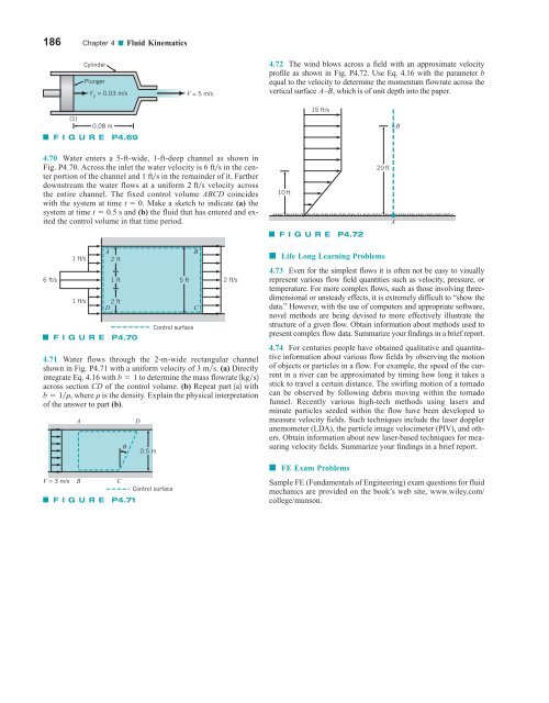
4.72 The wind blows across a field with an approximate velocity<br />
profile as shown in Fig. P4.72. Use Eq. 4.16 with the parameter b<br />
equal to the velocity to determine the momentum flowrate across the<br />
vertical surface A–B, which is of unit depth into the paper.<br />
(1)<br />
0.08 m<br />
F I G U R E P4.69<br />
15 ft/s<br />
B<br />
4.70 Water enters a 5-ft-wide, 1-ft-deep channel as shown in<br />
Fig. P4.70. Across the inlet the water velocity is 6 fts in the center<br />
portion of the channel and 1 fts in the remainder of it. Farther<br />
downstream the water flows at a uniform 2 fts velocity across<br />
the entire channel. The fixed control volume ABCD coincides<br />
with the system at time t 0. Make a sketch to indicate (a) the<br />
system at time t 0.5 s and (b) the <strong>fluid</strong> that has entered and exited<br />
the control volume in that time period.<br />
10 ft<br />
F I G U R E P4.72<br />
20 ft<br />
A<br />
1 ft/s<br />
6 ft/s<br />
1 ft/s<br />
A<br />
2 ft<br />
1 ft 5 ft<br />
2 ft<br />
D<br />
Control surface<br />
B<br />
2 ft/s<br />
C<br />
F I G U R E P4.70<br />
4.71 Water flows through the 2-m-wide rectangular channel<br />
shown in Fig. P4.71 with a uniform velocity of 3 ms. (a) Directly<br />
integrate Eq. 4.16 with b 1 to determine the mass flowrate 1kgs2<br />
across section CD of the control volume. (b) Repeat part 1a2 with<br />
b 1r, where r is the density. Explain the physical interpretation<br />
of the answer to part (b).<br />
A<br />
D<br />
θ<br />
0.5 m<br />
V = 3 m/s B<br />
C<br />
Control surface<br />
F I G U R E P4.71<br />
■ Life Long Learning Problems<br />
4.73 Even for the simplest flows it is often not be easy to visually<br />
represent various flow field quantities such as velocity, pressure, or<br />
temperature. For more complex flows, such as those involving threedimensional<br />
or unsteady effects, it is extremely difficult to “show the<br />
data.” However, with the use of computers and appropriate software,<br />
novel methods are being devised to more effectively illustrate the<br />
structure of a given flow. Obtain information about methods used to<br />
present complex flow data. Summarize your findings in a brief report.<br />
4.74 For centuries people have obtained qualitative and quantitative<br />
information about various flow fields by observing the motion<br />
of objects or particles in a flow. For example, the speed of the current<br />
in a river can be approximated by timing how long it takes a<br />
stick to travel a certain distance. The swirling motion of a tornado<br />
can be observed by following debris moving within the tornado<br />
funnel. Recently various high-tech methods using lasers and<br />
minute particles seeded within the flow have been developed to<br />
measure velocity fields. Such techniques include the laser doppler<br />
anemometer (LDA), the particle image velocimeter (PIV), and others.<br />
Obtain information about new laser-based techniques for measuring<br />
velocity fields. Summarize your findings in a brief report.<br />
■ FE Exam Problems<br />
Sample FE (Fundamentals of Engineering) exam questions for <strong>fluid</strong><br />
<strong>mechanics</strong> are provided on the book’s web site, www.wiley.com/<br />
college/munson.


