fluid_mechanics

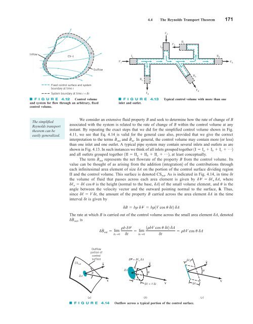
4.4 The Reynolds Transport Theorem 171
Inflow
CV–I
II
V 2
II c
V 3
I b
II b
II a
I a II d
V 5
V 1
V 6
V 4
I
Outflow
Fixed control surface and system
boundary at time t
System boundary at time t + δ t
F I G U R E 4.12 Control volume
and system for flow through an arbitrary, fixed
control volume.
F I G U R E 4.13
inlet and outlet.
Typical control volume with more than one
The simplified
Reynolds transport
theorem can be
easily generalized.
We consider an extensive fluid property B and seek to determine how the rate of change of B
associated with the system is related to the rate of change of B within the control volume at any
instant. By repeating the exact steps that we did for the simplified control volume shown in Fig.
4.11, we see that Eq. 4.14 is valid for the general case also, provided that we give the correct
interpretation to the terms B # and B # out in. In general, the control volume may contain more 1or less2
than one inlet and one outlet. A typical pipe system may contain several inlets and outlets as are
shown in Fig. 4.13. In such instances we think of all inlets grouped together
and all outlets grouped together
at least conceptually.
The term B # 1II II a II b II c p 1I I a I b I c p 2
2,
out represents the net flowrate of the property B from the control volume. Its
value can be thought of as arising from the addition 1integration2 of the contributions through
each infinitesimal area element of size dA on the portion of the control surface dividing region
II and the control volume. This surface is denoted CS out . As is indicated in Fig. 4.14, in time dt
the volume of fluid that passes across each area element is given by dV d/ n dA, where
d/ n d/ cos u is the height 1normal to the base, dA2 of the small volume element, and u is the
angle between the velocity vector and the outward pointing normal to the surface, nˆ . Thus,
since d/ V dt, the amount of the property B carried across the area element dA in the time
interval dt is given by
dB br dV br1V cos u dt2 dA
The rate at which B is carried out of the control volume across the small area element denoted
dB # dA,
out, is
dB # rb dV 1rbV cos u dt2 dA
out lim lim
rbV cos u dA
dtS0 dt dtS0 dt
CS out
Outflow
portion of
control
surface
^
n
δV = δ n δA
n^
δ n
^
n
δA
θ
δA
θ
θ
V
δ = V δt
V
δ
V
(a) (b) (c)
F I G U R E 4.14 Outflow across a typical portion of the control surface.