fluid_mechanics

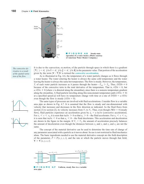
160 Chapter 4 ■ Fluid Kinematics
Water
heater
Hot
T out > T in
Pathline
___ ∂T
= 0
∂ t
DT ___
Dt
≠ 0
Cold
T in
F I G U R E 4.6 Steady-state
operation of a water heater. (Photo courtesy
of American Water Heater Company.)
u
0
a x
0
The convective derivative
is a result
of the spatial variation
of the flow.
x
x
It is due to the convection, or motion, of the particle through space in which there is a gradient
3 § 1 2 01 20x î 01 20y ĵ 01 20z kˆ4 in the parameter value. That portion of the acceleration
given by the term 1V § 2V is termed the convective acceleration.
As is illustrated in Fig. 4.6, the temperature of a water particle changes as it flows through
a water heater. The water entering the heater is always the same cold temperature and the water
leaving the heater is always the same hot temperature. The flow is steady. However, the temperature,
T, of each water particle increases as it passes through the heater— T out 7 T in . Thus, DTDt 0
because of the convective term in the total derivative of the temperature. That is, 0T0t 0, but
u 0T0x 0 1where x is directed along the streamline2, since there is a nonzero temperature gradient
along the streamline. A fluid particle traveling along this nonconstant temperature path 10T0x 02
at a specified speed 1u2 will have its temperature change with time at a rate of DTDt u 0T0x
even though the flow is steady 10T0t 02.
The same types of processes are involved with fluid accelerations. Consider flow in a variable
area pipe as shown in Fig. 4.7. It is assumed that the flow is steady and one-dimensional with
velocity that increases and decreases in the flow direction as indicated. As the fluid flows from
section 112 to section 122, its velocity increases from V 1 to V 2 . Thus, even though 0V0t 0 1steady
flow2, fluid particles experience an acceleration given by a x u 0u0x 1convective acceleration2.
For x 1 6 x 6 x 2 , it is seen that 0u0x 7 0 so that a x 7 0—the fluid accelerates. For x 2 6 x 6 x 3 ,
it is seen that 0u0x 6 0 so that a x 6 0—the fluid decelerates. This acceleration and deceleration
are shown in the figure in the margin. If V 1 V 3 , the amount of acceleration precisely balances
the amount of deceleration even though the distances between x 2 and x 1 and x 3 and x 2 are not the
same.
The concept of the material derivative can be used to determine the time rate of change of
any parameter associated with a particle as it moves about. Its use is not restricted to fluid mechanics
alone. The basic ingredients needed to use the material derivative concept are the field description
of the parameter, P P1x, y, z, t2, and the rate at which the particle moves through that field,
V V 1x, y, z, t2.
u = V 1
u = V 2 > V 1
x
x 2
1
F I G U R E 4.7
area pipe.
u = V 3 = V 1 < V 2
x 3
Uniform, steady flow in a variable
x