fluid_mechanics

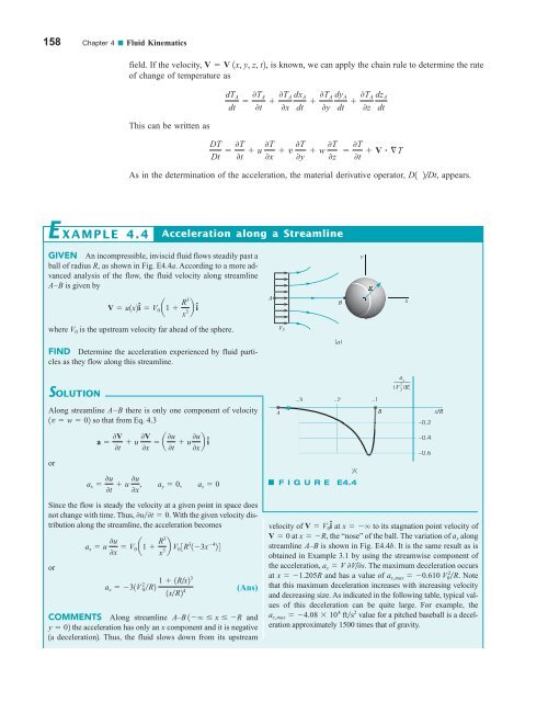
158 Chapter 4 ■ Fluid Kinematics
field. If the velocity, V V 1x, y, z, t2, is known, we can apply the chain rule to determine the rate
of change of temperature as
This can be written as
dT A
dt
0T A
0t
0T A dx A
0x dt
0T A dy A
0y dt
0T A dz A
0z dt
DT
Dt 0T
0t u 0T
0x v 0T
0y w 0T
0z 0T
0t V §T
As in the determination of the acceleration, the material derivative operator, D1 2Dt, appears.
E XAMPLE 4.4
Acceleration along a Streamline
GIVEN An incompressible, inviscid fluid flows steadily past a
ball of radius R, as shown in Fig. E4.4a. According to a more advanced
analysis of the flow, the fluid velocity along streamline
A–B is given by
y
V u1x2î V 0 a1 R3
x 3 b î
A
B
x
where
V 0
is the upstream velocity far ahead of the sphere.
V 0
FIND Determine the acceleration experienced by fluid particles
as they flow along this streamline.
(a)
SOLUTION
Along streamline A–B there is only one component of velocity
1v w 02 so that from Eq. 4.3
or
Since the flow is steady the velocity at a given point in space does
not change with time. Thus, 0u0t 0. With the given velocity distribution
along the streamline, the acceleration becomes
or
a 0V
0t
u 0V
0x a 0u
0t u 0u
0x b î
a x 0u
0t u 0u
0x , a y 0, a z 0
a x u 0u
0x V 0 a1 R3
x 3 b V 03R 3 13x 4 24
a x 31V 2
0 R2 1 1R x2 3
1xR2 4
(Ans)
COMMENTS Along streamline A–B 1q x R and
y 02 the acceleration has only an x component and it is negative
1a deceleration2. Thus, the fluid slows down from its upstream
A
–3
–2
(b)
F I G U R E E4.4
–1
B
_______ a x
/ )
(VV 2 0 /R
x/
R
–0.2
–0.4
–0.6
velocity of V V 0 î at x q to its stagnation point velocity of
V 0 at x R, the “nose” of the ball. The variation of a x along
streamline A–B is shown in Fig. E4.4b. It is the same result as is
obtained in Example 3.1 by using the streamwise component of
the acceleration, a x V 0V0s. The maximum deceleration occurs
at x 1.205R and has a value of a x,max 0.610 V 02 R. Note
that this maximum deceleration increases with increasing velocity
and decreasing size. As indicated in the following table, typical values
of this deceleration can be quite large. For example, the
a x,max 4.08 10 4 fts 2 value for a pitched baseball is a deceleration
approximately 1500 times that of gravity.