fluid_mechanics

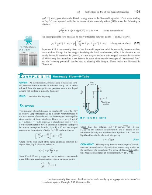
3.8 Restrictions on Use of the Bernoulli Equation 129
V3.11 Oscillations
in a U-tube
1
2 rd1V 2 2 term, gave rise to the kinetic energy term in the Bernoulli equation. If the steps leading
to Eq. 3.5 are repeated with the inclusion of the unsteady effect 10V0t 02 the following is
obtained:
r 0V
0t ds dp 1 2 rd1V 2 2 g dz 0
For incompressible flow this can be easily integrated between points 112 and 122 to give
p 1 1 2 rV 2 1 gz 1 r
s 2
s 1
0V
0t ds p 2 1 2 rV 2 2 gz 2
1along a streamline2
1along a streamline2
(3.27)
Equation 3.27 is an unsteady form of the Bernoulli equation valid for unsteady, incompressible,
inviscid flow. Except for the integral involving the local acceleration, 0V0t, it is identical to the
steady Bernoulli equation. In general, it is not easy to evaluate this integral because the variation
of 0V0t along the streamline is not known. In some situations the concepts of “irrotational flow”
and the “velocity potential” can be used to simplify this integral. These topics are discussed in
Chapter 6.
E XAMPLE 3.16
Unsteady Flow—U-Tube
GIVEN An incompressible, inviscid liquid is placed in a vertical,
constant diameter U-tube as indicated in Fig. E3.16. When
released from the nonequilibrium position shown, the liquid
column will oscillate at a specific frequency.
FIND
SOLUTION
Determine this frequency.
The frequency of oscillation can be calculated by use of Eq. 3.27
as follows. Let points 112 and 122 be at the air–water interfaces of
the two columns of the tube and z 0 correspond to the equilibrium
position of these interfaces. Hence, p 1 p 2 0 and if
z 2 z, then z 1 z. In general, z is a function of time, z z1t2.
For a constant diameter tube, at any instant in time the fluid speed
is constant throughout the tube, V 1 V 2 V, and the integral
representing the unsteady effect in Eq. 3.27 can be written as
s 2
s 1
0V dV
ds
0t dt s 2
where / is the total length of the liquid column as shown in the
figure. Thus, Eq. 3.27 can be written as
g1z2 r/ dV
dt gz
Since V dzdt and g rg, this can be written as the secondorder
differential equation describing simple harmonic motion
s 1
d 2 z
2
dt
2g
/ z 0
ds / dV
dt
g
Open
tube
V 2
(2)
z
z = 0
Equilibrium
(1)
position
V 1
F I G U R E E3.16
which has the solution z1t2 C 1 sin1 12g/ t2 C 2 cos
1 12g/ t2. The values of the constants C 1 and C 2 depend on the
initial state 1velocity and position2 of the liquid at t 0. Thus, the
liquid oscillates in the tube with a frequency
v 22g/
(Ans)
COMMENT This frequency depends on the length of the column
and the acceleration of gravity 1in a manner very similar to
the oscillation of a pendulum2. The period of this oscillation 1the
time required to complete an oscillation2 is t 0 2p1/2g.
In a few unsteady flow cases, the flow can be made steady by an appropriate selection of the
coordinate system. Example 3.17 illustrates this.