fluid_mechanics

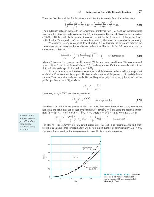
3.8 Restrictions on Use of the Bernoulli Equation 127
Thus, the final form of Eq. 3.6 for compressible, isentropic, steady flow of a perfect gas is
k
a
k 1 b p 1
V 2 1
r 1 2 gz k
1 a
k 1 b p 2
V 2 2
r 2 2 gz 2
(3.24)
The similarities between the results for compressible isentropic flow 1Eq. 3.242 and incompressible
isentropic flow 1the Bernoulli equation, Eq. 3.72 are apparent. The only differences are the factors
of 3k1k 124 that multiply the pressure terms and the fact that the densities are different 1r 1 r 2 2.
In the limit of “low-speed flow” the two results are exactly the same, as is seen by the following.
We consider the stagnation point flow of Section 3.5 to illustrate the difference between the
incompressible and compressible results. As is shown in Chapter 11, Eq. 3.24 can be written in
dimensionless form as
p 2 p 1
ca1 k 1 kk1
Ma 2
p
1b 1 d
1 2
1compressible2
(3.25)
where 112 denotes the upstream conditions and 122 the stagnation conditions. We have assumed
z 1 z 2 , V 2 0, and have denoted Ma 1 V 1c 1 as the upstream Mach number—the ratio of the
fluid velocity to the speed of sound, c 1 1kRT 1 .
A comparison between this compressible result and the incompressible result is perhaps most
easily seen if we write the incompressible flow result in terms of the pressure ratio and the Mach
number. Thus, we divide each term in the Bernoulli equation, rV 12 2 p 1 p 2 , by p 1 and use the
perfect gas law, p 1 rRT 1 , to obtain
p 2 p 1
V 2 1
p 1 2RT 1
Since Ma 1 V 1 1kRT 1 this can be written as
p 2 p 1
p 1
kMa2 1
2
1incompressible2
(3.26)
For small Mach
numbers the compressible
and incompressible
results are nearly
the same.
Equations 3.25 and 3.26 are plotted in Fig. 3.24. In the low-speed limit of both of the
results are the same. This can be seen by denoting
and using the binomial expansion,
11 ~ e 2 n 1 ne ~ n1n 12 ~2 e 2 p 1k 12Ma 12 2 e ~ Ma 1 S 0,
, where n k1k 12, to write Eq. 3.25 as
p 2 p 1
kMa2 1
a1 1 p 1 2 4 Ma2 1 2 k
24 Ma4 1 p b 1compressible2
For Ma 1 1 this compressible flow result agrees with Eq. 3.26. The incompressible and compressible
equations agree to within about 2% up to a Mach number of approximately Ma 1 0.3.
For larger Mach numbers the disagreement between the two results increases.
1
0.8
0.6
Compressible
(Eq. 3.25)
______ p 2
– p 1
p 1
0.4
k = 1.4
0.2
Incompressible
(Eq. 3.26)
0
0 0.2 0.4 0.6 0.8 1
Ma 1
F I G U R E 3.24 Pressure
ratio as a function of Mach number
for incompressible and compressible
(isentropic) flow.