fluid_mechanics

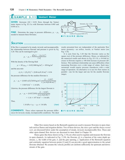
120 Chapter 3 ■ Elementary Fluid Dynamics—The Bernoulli Equation
E XAMPLE 3.11
Venturi Meter
GIVEN Kerosene 1SG 0.852 flows through the Venturi
meter shown in Fig. E3.11a with flowrates between 0.005 and
0.050 m 3 s.
FIND Determine the range in pressure difference, p 1 p 2 ,
needed to measure these flowrates.
Kerosene, SG = 0.85
D 1 = 0.1 m
(2) D 2 = 0.06 m
(1)
0.005 m 3 /s < Q < 0.050 m 3 /s
F I G U R E E3.11a
Q
SOLUTION
If the flow is assumed to be steady, inviscid, and incompressible,
the relationship between flowrate and pressure is given by Eq.
3.20. This can be rearranged to give
With the density of the flowing fluid
and the area ratio
the pressure difference for the smallest flowrate is
Likewise, the pressure difference for the largest flowrate is
Thus,
p 1 p 2 Q2 r31 1A 2A 1 2 2 4
2 A 2 2
r SG r H2 O 0.8511000 kgm 3 2 850 kgm 3
A 2A 1 1D 2D 1 2 2 10.06 m0.10 m2 2 0.36
11 0.36 2 2
p 1 p 2 10.005 m 3 s2 2 1850 kgm 3 2
2 31p4210.06 m2 2 4 2
1160 Nm 2 1.16 kPa
11 0.36 2 2
p 1 p 2 10.052 2 18502
231p4210.062 2 4 2
1.16 10 5 Nm 2 116 kPa
1.16 kPa p 1 p 2 116 kPa
(Ans)
COMMENTS These values represent the pressure differences
for inviscid, steady, incompressible conditions. The ideal
results presented here are independent of the particular flow
meter geometry—an orifice, nozzle, or Venturi meter 1see
Fig. 3.182.
It is seen from Eq. 3.20 that the flowrate varies as the
square root of the pressure difference. Hence, as indicated by
the numerical results and shown in Fig. E3.11b, a 10-fold increase
in flowrate requires a 100-fold increase in pressure difference.
This nonlinear relationship can cause difficulties when
measuring flowrates over a wide range of values. Such measurements
would require pressure transducers with a wide
range of operation. An alternative is to use two flow meters in
parallel—one for the larger and one for the smaller flowrate
ranges.
p 1
–p 2 , kPa
120
100
80
60
40
20
0
0
(0.005 m 3 /s, 1.16 kPa)
F I G U R E E3.11b
(0.05 m 3 /s, 116 kPa)
0.01 0.02 0.03 0.04 0.05
Q, m 3 /s
Other flow meters based on the Bernoulli equation are used to measure flowrates in open channels
such as flumes and irrigation ditches. Two of these devices, the sluice gate and the sharp-crested
weir, are discussed below under the assumption of steady, inviscid, incompressible flow. These and
other open-channel flow devices are discussed in more detail in Chapter 10.
Sluice gates like those shown in Fig. 3.19a are often used to regulate and measure the flowrate
in open channels. As indicated in Fig. 3.19b, the flowrate, Q, is a function of the water depth upstream,
z 1 , the width of the gate, b, and the gate opening, a. Application of the Bernoulli equation
and continuity equation between points 112 and 122 can provide a good approximation to the actual
flowrate obtained. We assume the velocity profiles are uniform sufficiently far upstream and downstream
of the gate.