fluid_mechanics

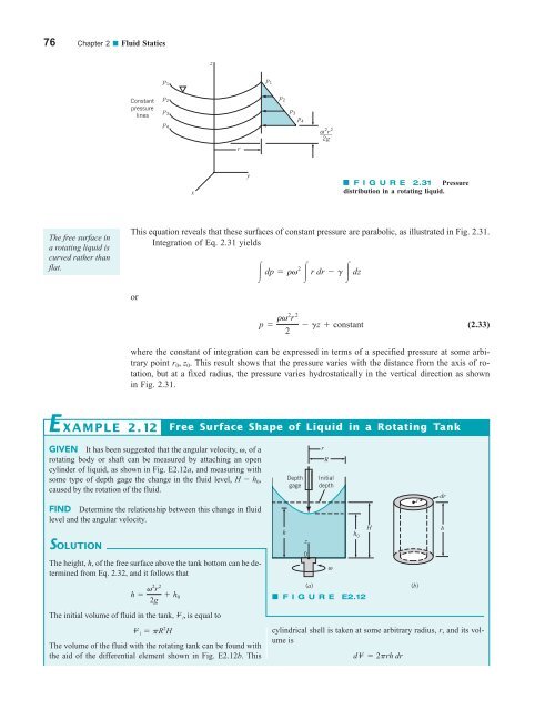
76 Chapter 2 ■ Fluid Statics
z
p 1
Constant
pressure
lines
p 2
p 3
p 1
p 2
p 3
p4
p 4
____ ω
2 r 2
2g
r
x
y
F I G U R E 2.31 Pressure
distribution in a rotating liquid.
The free surface in
a rotating liquid is
curved rather than
flat.
This equation reveals that these surfaces of constant pressure are parabolic, as illustrated in Fig. 2.31.
Integration of Eq. 2.31 yields
dp rv2 r dr g dz
or
p rv2 r 2
gz constant
2
(2.33)
where the constant of integration can be expressed in terms of a specified pressure at some arbitrary
point r 0 , z 0 . This result shows that the pressure varies with the distance from the axis of rotation,
but at a fixed radius, the pressure varies hydrostatically in the vertical direction as shown
in Fig. 2.31.
E XAMPLE 2.12
Free Surface Shape of Liquid in a Rotating Tank
GIVEN It has been suggested that the angular velocity, v, of a
rotating body or shaft can be measured by attaching an open
cylinder of liquid, as shown in Fig. E2.12a, and measuring with
some type of depth gage the change in the fluid level, H h 0 ,
caused by the rotation of the fluid.
FIND Determine the relationship between this change in fluid
level and the angular velocity.
SOLUTION
The height, h, of the free surface above the tank bottom can be determined
from Eq. 2.32, and it follows that
h v2 r 2
2g h 0
The initial volume of fluid in the tank, V i , is equal to
V i pR 2 H
The volume of the fluid with the rotating tank can be found with
the aid of the differential element shown in Fig. E2.12b. This
h
Depth
gage
z
0
r
R
Initial
depth
ω
h 0
(a)
F I G U R E E2.12
H
cylindrical shell is taken at some arbitrary radius, r, and its volume
is
dV2prh dr
r
(b)
dr
h