

Energy_slides

You also want an ePaper? Increase the reach of your titles
YUMPU automatically turns print PDFs into web optimized ePapers that Google loves.
M. Vable Intermediate Mechanics of Materials: Chapter 7<br />
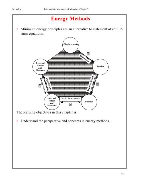
<strong>Energy</strong> Methods<br />
• Minimum-energy principles are an alternative to statement of equilibrium<br />
equations.<br />
Displacements<br />
1<br />
Kinematics<br />
External<br />
Forces<br />
and<br />
Moments<br />
Strains<br />
4<br />
<strong>Energy</strong> Methods<br />
Equilibrium<br />
Material Models<br />
2<br />
Internal<br />
Forces<br />
and<br />
Moments<br />
Static Equivalency<br />
3<br />
Stresses<br />
The learning objectives in this chapter is:<br />
• Understand the perspective and concepts in energy methods.<br />
7-1
M. Vable Intermediate Mechanics of Materials: Chapter 7<br />
Strain <strong>Energy</strong><br />
• The energy stored in a body due to deformation is called the strain<br />
energy.<br />
• The strain energy per unit volume is called the strain energy density<br />
and is the area underneath the stress-strain curve up to the point of<br />
deformation.<br />
σ<br />
U o = Complimentary strain energy den<br />
dU o = ε dσ<br />
A<br />
dσ<br />
U o = Strain energy density<br />
O<br />
dε<br />
Strain <strong>Energy</strong>: U = U o dV<br />
[<br />
V<br />
ε<br />
Strain <strong>Energy</strong> Density: U o<br />
= ∫σdε<br />
0<br />
Units: N-m / m 3 , Joules / m 3 , in-lbs / in 3 , or ft-lb/ft. 3<br />
Complimentary Strain <strong>Energy</strong> Density:<br />
dU o = σ dε<br />
∫<br />
U o<br />
=<br />
σ<br />
∫<br />
0<br />
εdσ<br />
ε<br />
7-2
M. Vable Intermediate Mechanics of Materials: Chapter 7<br />
Uniaxial tension test:<br />
Linear Strain <strong>Energy</strong> Density<br />
U o<br />
ε ε<br />
Eε 2<br />
= ∫σdε<br />
= ∫( Eε) dε<br />
= -------- =<br />
2<br />
0 0<br />
1<br />
--σε<br />
2<br />
1<br />
U o<br />
= --τγ<br />
2<br />
• Strain energy and strain energy density is a scaler quantity.<br />
1<br />
U o<br />
= -- [ σ<br />
2 xx<br />
ε xx<br />
+ σ yy<br />
ε yy<br />
+ σ zz<br />
ε zz<br />
+ τ xy<br />
γ xy<br />
+ τ yz<br />
γ yz<br />
+ τ zx<br />
γ zx<br />
]<br />
1-D Structural Elements<br />
y<br />
A<br />
z<br />
x<br />
dx<br />
dV=Adx<br />
Axial strain energy<br />
• All stress components except σ xx are zero.<br />
σ xx<br />
du ( x)<br />
= Eε xx<br />
ε xx =<br />
dx<br />
1 2 1<br />
U A ∫<br />
--Eε<br />
2 xx dV --E ⎛du⎞ 2 = = ∫ ∫ dA<br />
dx<br />
=<br />
2 ⎝ dx<br />
⎠<br />
V<br />
• U a is the strain energy per unit length.<br />
L<br />
A<br />
1<br />
U A<br />
= ∫U a<br />
dx<br />
U a<br />
--EA⎛du⎞ 2<br />
=<br />
2 ⎝ dx<br />
⎠<br />
L<br />
∫<br />
L<br />
1 du<br />
--<br />
2⎝<br />
⎛ dx⎠<br />
⎞ 2 ∫ E d A<br />
A<br />
dx<br />
1<br />
U A = ∫U a dx<br />
U a = ---------<br />
N2<br />
2EA<br />
L<br />
7-3
M. Vable Intermediate Mechanics of Materials: Chapter 7<br />
Torsional strain energy<br />
• All stress components except τ xθ in polar coordinate are zero<br />
τ xθ<br />
= Gγ xθ<br />
γ xθ = ρ x<br />
dφ ( x)<br />
d<br />
1 2 1<br />
U T ∫<br />
--Gγ<br />
2 xθ<br />
dV<br />
2<br />
--G ⎛ ρ dφ⎞ 2 = = ∫ ∫ dA<br />
dx<br />
=<br />
⎝ d x ⎠<br />
V<br />
• U t is the strain energy per unit length.<br />
L<br />
A<br />
1<br />
U T<br />
= ∫U t<br />
dx<br />
U t<br />
--GJ⎛dφ⎞ 2<br />
=<br />
2 ⎝dx⎠<br />
L<br />
∫<br />
L<br />
1 dφ<br />
--<br />
2⎝<br />
⎛ dx⎠<br />
⎞ 2 ∫ Gρ 2 d A<br />
A<br />
dx<br />
1<br />
U T = ∫U t dx<br />
U t = -- -------<br />
T2<br />
2GJ<br />
Strain energy in symmetric bending about z-axis<br />
There are two non-zero stress components, σ xx and τ xy.<br />
σ xx<br />
L<br />
d v<br />
= Eε xx ε xx = – y<br />
dx 2<br />
2<br />
1 2 1 ⎛ d v ⎞ 2<br />
U B = ∫<br />
--Eε<br />
2 xx dV = ∫ ∫<br />
--E⎜y<br />
2 ⎝ dx 2 ⎟ dA<br />
dx<br />
=<br />
⎠<br />
V<br />
L<br />
A<br />
• where U b is the bending strain energy per unit length.<br />
2<br />
2<br />
1 ⎛d v ⎞ 2<br />
U B = ∫U b dx<br />
U b = --EI<br />
2 zz ⎜<br />
⎝dx 2 ⎟<br />
⎠<br />
L<br />
∫<br />
L<br />
2<br />
1⎛d v ⎞ 2<br />
-- ⎜<br />
2⎝dx 2 ⎟ ∫ Ey 2 dA<br />
⎠<br />
A<br />
dx<br />
The strain energy due to shear in bending is:<br />
As<br />
τ max<br />
2<br />
1<br />
M z<br />
U B = ∫U b dx<br />
U b = -- ----------<br />
2<br />
L<br />
EI zz<br />
« σ max<br />
U s<br />
« U B<br />
1<br />
U S =<br />
∫<br />
--τ<br />
2 xy γ xy dV<br />
=<br />
V<br />
1<br />
-- τ 2<br />
xy<br />
∫<br />
------ dV<br />
2 E<br />
V<br />
7-4
M. Vable Intermediate Mechanics of Materials: Chapter 7<br />
Table 7.1 <strong>Energy</strong> densities<br />
Axial<br />
Torsion of circular<br />
shafts<br />
Symmetric<br />
bending of<br />
beams<br />
Strain energy density per<br />
unit length<br />
Complimentary strain<br />
energy density per unit<br />
length<br />
1 du<br />
U a = --EA⎛ ⎞ 2<br />
1<br />
2 ⎝ dx<br />
⎠ U a = ---------<br />
N2<br />
2EA<br />
1 dφ<br />
U t<br />
= --GJ⎛ ⎞ 2<br />
1<br />
2 ⎝dx⎠<br />
U t = -- -------<br />
T2<br />
2GJ<br />
2<br />
1 ⎛d v ⎞ 2<br />
1<br />
U b<br />
= --EI<br />
2 zz ⎜<br />
⎝dx 2 ⎟ U b -- M 2<br />
z<br />
= ----------<br />
⎠<br />
2EI zz<br />
7-5
M. Vable Intermediate Mechanics of Materials: Chapter 7<br />
Work<br />
• If a force moves through a distance, then work has been done by the<br />
force.<br />
• Work done by a force is conservative if it is path independent.<br />
• Non-linear systems and non-conservative systems are two independent<br />
description of a system.<br />
Loading Mode<br />
P<br />
dW<br />
=<br />
Fdu<br />
δW<br />
Work<br />
=<br />
Pδu L<br />
p(x)<br />
u(x)<br />
u L<br />
δW<br />
=<br />
L<br />
∫<br />
0<br />
p( x)δux<br />
( ) dx<br />
T<br />
δW<br />
=<br />
Tδφ L<br />
t (x)<br />
φ( x)<br />
φ L<br />
δW<br />
=<br />
L<br />
∫<br />
0<br />
t( x)δφ( x) dx<br />
δW<br />
=<br />
Pδv L<br />
P<br />
M<br />
v L<br />
θ<br />
=<br />
dv<br />
dx<br />
δW<br />
=<br />
Mδθ L<br />
v(x)<br />
δW<br />
=<br />
L<br />
∫<br />
0<br />
p( x)δvx<br />
( ) dx<br />
p(x)<br />
• Any variable that can be used for describing deformation is called the<br />
generalized displacement.<br />
• Any variable that can be used for describing the cause that produces<br />
deformation is called the generalized force.<br />
7-6
M. Vable Intermediate Mechanics of Materials: Chapter 7<br />
Virtual Work<br />
• Virtual work methods are applicable to linear and non-linear systems,<br />
to conservative as well as non-conservative systems.<br />
The principle of virtual work:<br />
The total virtual work done on a body at equilibrium is zero.<br />
δW = 0<br />
• Symbol δ will be used to designate a virtual quantity<br />
δW ext = δW int<br />
Types of boundary conditions<br />
y Displacement and rotation specified<br />
at this end<br />
T<br />
x<br />
P x<br />
Internal forces and moment specified<br />
at this end to meet equilibrium<br />
T<br />
N<br />
V y<br />
T<br />
P x<br />
z<br />
M<br />
ε<br />
P y M<br />
ε<br />
P y<br />
Kinematic variable<br />
Statical variable<br />
(Primary variable)<br />
(Secondary variable)<br />
or<br />
u<br />
N<br />
φ<br />
or<br />
T<br />
v<br />
or<br />
θ<br />
Geometric boundary conditions (Kinematic boundary conditions)<br />
(Essential boundary conditions):<br />
Condition specified on kinematic (primary) variable at the boundary.<br />
Statical boundary conditions<br />
(Natural boundary conditions)<br />
Condition specified on statical (secondary)variable at the boundary.<br />
M z<br />
V y<br />
dv<br />
=<br />
or<br />
M<br />
dx<br />
z<br />
7-7
M. Vable Intermediate Mechanics of Materials: Chapter 7<br />
Kinematically admissible functions<br />
• Functions that are continuous and satisfies all the kinematic boundary<br />
conditions are called kinematically admissible functions.<br />
• actual displacement solution is always a kinematically admissible<br />
function<br />
• Kinematically admissible functions are not required to correspond to<br />
solutions that satisfy equilibrium equations.<br />
Statically admissible functions<br />
• Functions that satisfy satisfies all the static boundary conditions, satisfy<br />
equilibrium equations at all points, and are continuous at all points<br />
except where a concentrated force or moment is applied are called<br />
statically admissible functions.<br />
• Actual internal forces and moments are always statically admissible.<br />
• Statically admissible functions are not required to correspond to solutions<br />
that satisfy compatibility equations.<br />
7.3 Determine a class of kinematically admissible displacement<br />
functions for the beam shown in Fig. P7.3.<br />
A<br />
x<br />
L<br />
Fig. P7.3<br />
7.4 For the beam and loading shown in Fig. P7.3 determine a statically<br />
admissible bending moment.<br />
B<br />
wL 2<br />
w<br />
L<br />
C<br />
7-8
M. Vable Intermediate Mechanics of Materials: Chapter 7<br />
Virtual displacement method<br />
• The virtual displacement is an infinitesimal imaginary kinematically<br />
admissible displacement field imposed on a body.<br />
actual displacement<br />
x<br />
kinematically admissible displacement<br />
δv = virtual displacement<br />
• Of all the virtual displacements the one that satisfies the virtual work<br />
principle is the actual displacement field.<br />
Virtual Force Method<br />
• The virtual force is an infinitesimal imaginary statically admissible<br />
force field imposed on a body.<br />
• Of all the virtual force fields the one that satisfies the virtual work<br />
principle is the actual force field.<br />
7-9
M. Vable Intermediate Mechanics of Materials: Chapter 7<br />
7.7 The roller at P shown in Fig. P7.7 <strong>slides</strong> in the slot due to the<br />
force F = 20kN. Both bars have a cross-sectional area of A = 100 mm 2<br />
and a modulus of elasticity E = 200 GPa. Bar AP and BP have lengths of<br />
L AP = 200 mm and L BP = 250 mm respectively. Determine the axial stress<br />
in the member AP by virtual displacement method.<br />
B<br />
A<br />
110 o F<br />
Fig. P7.7<br />
7.8 A force F = 20kN is appled to pin shown in Fig. P7.8. Both<br />
bars have a cross-sectional area of A = 100 mm 2 and a modulus of elasticity<br />
E = 200 GPa. Bar AP and BP have lengths of L AP = 200 mm and<br />
L BP = 250 mm respectively. Using virtual force method determine the<br />
movement of pin in the direction of force F.<br />
P<br />
B<br />
A<br />
110 o P<br />
F<br />
40 o<br />
Fig. P7.8<br />
7-10