Mode degeneracies and the Petermann excess-noise factor for ...

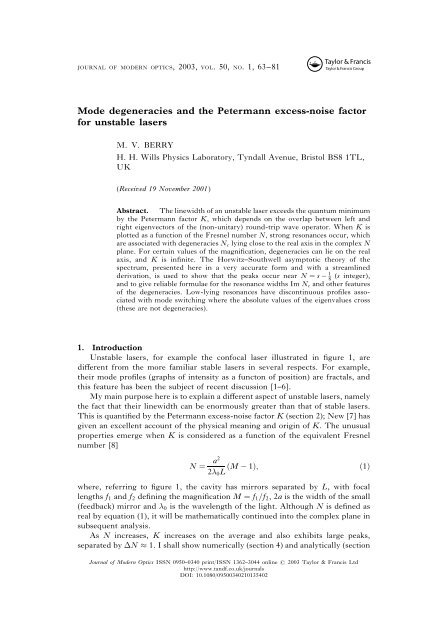
journal of modern optics, 2003, vol. 50, no. 1, 63–81 

Mode degeneracies and the Petermann excess-noise factor 

for unstable lasers 

M. V. BERRY 

H. H. Wills Physics Laboratory, Tyndall Avenue, Bristol BS81TL, 

UK 

(Received 19 November 2001) 

Abstract. The linewidth of an unstable laser exceeds the quantum minimum 

by the Petermann factor K, which depends on the overlap between left and 

right eigenvectors of the (non-unitary) round-trip wave operator. When K is 

plotted as a function of the Fresnel number N, strong resonances occur, which 

are associated with degeneracies Nc lying close to the real axis in the complex N 

plane. For certain values of the magnification, degeneracies can lie on the real 

axis, and K is infinite. The Horwitz–Southwell asymptotic theory of the 

spectrum, presented here in a very accurate form and with a streamlined 

1 

derivation, is used to show that the peaks occur near N ¼ s 8 (s integer), 

and to give reliable formulae for the resonance widths Im Nc and other features 

of the degeneracies. Low-lying resonances have discontinuous profiles associated 

with mode switching where the absolute values of the eigenvalues cross 

(these are not degeneracies). 

1. Introduction 

Unstable lasers, for example the confocal laser illustrated in figure 1, are 

different from the more familiar stable lasers in several respects. For example, 

their mode profiles (graphs of intensity as a functon of position) are fractals, and 

this feature has been the subject of recent discussion [1–6]. 

My main purpose here is to explain a different aspect of unstable lasers, namely 

the fact that their linewidth can be enormously greater than that of stable lasers. 

This is quantified by the Petermann excess-noise factor K (section 2); New [7] has 

given an excellent account of the physical meaning and origin of K. The unusual 

properties emerge when K is considered as a function of the equivalent Fresnel 

number [8] 

N ¼ a2 

ðM1Þ; ð1Þ 

2 0L 

where, referring to figure 1, the cavity has mirrors separated by L, with focal 

lengths f1 and f2 defining the magnification M ¼ f1=f2, 2a is the width of the small 

(feedback) mirror and 0 is the wavelength of the light. Although N is defined as 

real by equation (1), it will be mathematically continued into the complex plane in 

subsequent analysis. 

As N increases, K increases on the average and also exhibits large peaks, 

separated by N 1. I shall show numerically (section 4) and analytically (section 

Journal of Modern Optics ISSN 0950–0340 print/ISSN 1362–3044 online # 2003 Taylor & Francis Ltd 

http://www.tandf.co.uk/journals 

DOI: 10.1080/09500340210135402

64 M. V. Berry 

5) that these peaks are resonances, associated with degeneracies where the complex 

lowest-loss mode eigenvalue is degenerate with that of the next-lowest-loss 

mode. The degeneracies occur at points Nc in the complex N plane, near 

N ¼ s 1 

Figure 1. Strip resonator cavity corresponding to a confocal unstable laser. 

8 

(s integer) on the real axis and close to a curve whose form will be 

calculated explicitly. For general magnification M, there is zero probability that 

degeneracies will occur precisely on the real axis. However, for certain values of 

M, one of which is given explicitly, this can occur, and then K !1. 

It is important to distinguish degeneracies from eigenvalue crossings, which 

1 

occur on the real N axis close (once again) to the points N ¼ s 8 . Whereas the 

lowest- and next-lowest-loss mode eigenvalues are identical at the degeneracies, 

only their moduli j j coincide at the crossings [8, 9]. It must be stressed that it is 

the degeneracies, and not the crossings, that are responsible for the large values of 

the Petermann factor. The crossings give rise to peculiar resonance shapes for 

small N (section 6). 

This theory of K will be derived with the aid of a slight modification (section 3) 

of a beautiful and powerful large-N asymptotic theory of unstable laser modes, 

created by Horwitz [9] and Southwell [10]. Two subsidiary purposes of this paper 

are to give a derivation of this asymptotic theory that displays its structure in a 

simple way, and to demonstrate its very high accuracy, even for N 1. In some 

numerical applications, versions of the Horwitz–Southwell theory have been used 

as the basis of further refinements (e.g. by iteration), but the version here is so 

accurate that this is not necessary. 

From a mathematical point of view, unstable lasers are interesting because their 

characteristic properties depend on the fact that the operator governing their 

modes is non-unitary. As will become clear, the contrast with unitary operators 

becomes extreme in the neighbourhood of degeneracies. Therefore K essentially 

embodies the physics of non-unitarity, and, because the degeneracies dominating

K occur for complex N, the Petermann factor represents ‘real physics in the 

complex plane’. Excess noise joins a growing group of phenomena depending on 

degeneracies of non-unitary (or non-Hermitian) operators. Others include propagation 

near the optic axes of absorbing anisotropic crystals [11, 12], and the 

diffraction of atomic beams by crystals of light [13, 14]. 

To bring out the main ideas as clearly as possible, the theory of this paper is 

restricted to strip resonators, where (figure 1) the cavity is two dimensional and the 

mirrors are one dimensional. Calculations for more realistic three-dimensional 

cavities [15] have shown that K depends strongly on the shape of the mirrors. 

However, the underlying reason for the large values of K is the same as for strip 

resonators, namely degeneracies. 

2. Basics 

The lowest-loss mode profile uðxÞ in any plane, for example close to the small 

mirror, can be regarded as an eigenvector jui of an operator ^T representing wave 

propagation in a round trip of the cavity: 

^Tjui ¼ jui; hxjui ux ð Þ: ð2Þ 

For unstable lasers, losses at the edges of the mirrors make ^T non-unitary, so that 

j j < 1. Therefore its right eigenvectors jui are different from the left eigenvectors 

hvj, defined, together with the corresponding profile vðxÞ, by 

that is 

Petermann factor for unstable lasers 65 

hvj ^T ¼ hvj; hvjxi vðxÞ; 

^T y jvi ¼ jvi; hxjvi ¼v ðxÞ: ð3Þ 

The Petermann factor that will be the focus of our interest here can now be defined 

in terms of the ‘self-overlap’ between the right and left eigenvectors, by 

K ¼ uju h ihvjvi jhujvij 2 : ð4Þ 

Here and hereafter we shall measure positions in the plane of the feedback 

mirror in units of a. Then the explicit form of the round-trip operator is [8] 

1=2 

hxj ^T 

2N 

jyi ¼ 

i M M 1 

2pN x 2 

exp i y Yð1jyjÞ; ð5Þ 

ð Þ 1 M 2 M 

where Y denotes the unit step (without this step, cutting off the reflection at the 

edges of the mirror, ^T would be unitary). (Although equation (5) is written for a 

confocal laser, the operator for any unstable laser can be written in the same form, 

after a simple transformation involving a phase factor quadratic in x.) 

From the integral equation (12) below corresponding to equation (5), elementary 

manipulations show that for this particular operator vðxÞ and uðxÞ are related 

by [16] 

vx ð Þ ¼ ux ð Þexp 2piNx 2 Yð1jxjÞ: ð6Þ 

Thus vðxÞ is non-zero only in the interval jxj < 1 corresponding to the mirror, 

unlike uðxÞ whose domain extends outside the mirror, that is for jxj > 1. Never-


theless, the normalization of uðxÞ, that occurs in the definition (4) of K, can be 

expressed as an integral only over the interval jxj < 1; in appendix A it is shown 

that 

ð1 hvjvi ¼ dxjuðxÞj 

1 

2 ð1 ; hujui ¼ dx juðxÞj 

1 

2 ¼ 1 

j j 2 

ð1 dx juðxÞj 

1 

2 : ð7Þ 

Thus the Petermann factor can be written in the form 

K ¼ 

j j 2 

ð 1 

ð 1 

dxjuðxÞj 

1 

2 

dxu 

1 

2 ðxÞ exp ð2piNx 2 Þ 

2 

: ð8Þ 

2 

If the operator ^T were unitary, we would have vðxÞ ¼u ðxÞ and j j¼1, and the 

self-overlap in equation (4), and hence K, would both be unity. The extreme 

antithesis occurs at degeneracies; there the self-overlap is zero, and so K is infinite. 

To see this, and to motivate our later emphasis on degeneracies, consider the 

general 2 2 matrix 

T ¼ 

a b 

c d 

; ð9Þ 

where a, b, c and d can be complex. Labelling the two states þ and , the 

eigenvalues are 

¼ 1 

2 

a þ d " ð Þ; " ¼ þ ¼½ða dÞ 2 þ 4bcŠ 1=2 ; ð10Þ 

where " denotes the eigenvalue difference, so that a degeneracy corresponds to 

" ¼ 0. In appendix B it is shown that near a degeneracy the self-overlap (the same 

for both normalized states for a 2 2 matrix) is 

jhvjuij ! j"j 

as " ! 0: ð11Þ 

jbjþjcj 

Thusjui and hvj become orthogonal at a degeneracy, and K indeed diverges. Later 

we shall explore the full consequences of this. 

3. Reprise of Horwitz–Southwell asymptotics 

Corresponding to the operator equation (2) is the integral equation 

1=2ð 1 

uðxÞ ¼hxj^Tjui 2N 

¼ 

iðM M 1 2pN x 2 

dy exp i y uðyÞ; ð12Þ 

Þ 1 1 M 2 M 

which will be the basis of our subsequent analysis. To obtain a preliminary 

orientation, consider the crude approximation of taking uðxÞ as a constant and 

regarding the limits of integration as infinite. This gives 

and so 

uðxÞ 1; hxj ^Tjui 

1 

; 

M1=2

1 

; 

M1=2 ð13Þ 

motivating the definition of the scaled eigenvalue , defined by 

: ð14Þ 

M1=2 Horwitz [9] asymptotics is based on the mathematical observation that for large 

N the integrand in equation (12) oscillates rapidly, and the main contributions 

come from any stationary-phase points in the range of integration |x|


where again the first and second terms on the right-hand side correspond to 

geometrically reflected and edge-diffracted waves respectively. 

These two equations can be regarded as approximations to the integral operator 

^T. It is remarkable that the corresponding eigenequation, approximating equation 

(12), can be solved exactly (appendix C), with the result that the modes even 

in x are given by 

uðxÞ ¼1 X1 

n¼1 

where the scaled eigenvalues are the solutions of 

P ð ; NÞ 

¼ 1 þ G1ð1Þþ X1 Gnþ1 1 

n¼1 

GnðxÞ Gnð1Þ 

n ; ð18Þ 

ð Þ Gn 1 

ð Þ 

n ¼ 0: ð19Þ 

The function Pð ; NÞ is essentially the determinant of the (approximated) operator 

(5). The lowest-loss mode is the one (or two, in the case of a crossing) with the 

largest value of j j. 

The series in equations (18) and (19) are very convenient for numerical 

evaluation, because they converge very rapidly, as can be seen from the asymptotic 

forms 

Gnð1Þ 

exp½2piðN þ 1 

8ÞŠ pð2NÞ 1=2 

1 

exp½2piðN þ 

G1ð1Þ ¼G1ðxÞ ¼ 

cos 4pN 

M n if n 1orM 1; 


The number of terms required for convergence is of the order of 

log N 

mmax ¼ ð21Þ 

log M: 

Note the factors exp ½2piðN þ 1 

8ÞŠ; these are positive real whenever N ¼ s 1 

8 , 

values close to the maxima of K, as will be shown later. 

Figure 2 shows the Petermann factor for the lowest-loss mode, for rather small 

values of N. The computations were made according to equation (8), in two ways: 

: 

ð20Þ 

Figure 2. Petermann factor for the lowest-loss mode, for M ¼ 1:5, computed exactly, by 

matrix diagonalization (——), and according to the asymptotic theory (——).

firstly, using the exact modes, calculated by diagonalizing the matrix obtained by 

discretizing the integral operator in equation (12) and, secondly, using the 

1 

approximate modes (18). The large values near N ¼ s 8 , which we seek to 

explain, are clear, as is the excellent agreement, improving as N increases, between 

the asymptotic and exact theories. Figure 2 also agrees very closely with a 

previously published exact calculation [16]. The corresponding spectra, in the 

form of absolute values j j of the eigenvalues for the three lowest-loss modes, are 

shown in figure 3; again the asymptotic theory improves with increasing N, 

especially for the lowest-loss mode that is our main interest here. More discriminating 

are the eigenfunctions uðxÞ, whose absolute values are shown in figure 4; 

again the asymptotic theory gives excellent agreement with exact calculations. 

Further calculations, not reported here, confirm the accuracy of the asymptotic 

theory. One example is M ¼ 1:9, N ¼ 49:4, for which New [7] calculated K 290 

from the exact round-trip wave map; from the asymptotic theory, we obtain 

K ¼ 289:477. Thus we can have full confidence in a theory of the resonances based 

on the asymptotic theory. 

4. Fine structure of degeneracies 

According to equation (10), a degeneracy, that is vanishing ", requires both the 

real and the imaginary parts of the square root in equation (10) to vanish; therefore 

degeneracies have codimension two, a result that holds for a general complex 

matrix. This implies that degeneracies are infinitely unlikely to occur as a single 

real parameter, for example N, is varied, but can occur in the complex plane of N. 

Equations (4) and (11) then show that K will diverge as 1=j"j 2 . Now we shall 

examine this behaviour in detail. 

Let a degeneracy occur at the complex Fresnel number N ¼ Nc where the 

scaled eigenvalue is c. This situation corresponds to a double zero of the 

determinant function Pð ; NÞ, given by equation (19) according to the asymptotic 

theory. Thus (denoting derivatives by q) 

Pð c; NcÞ ¼0 and q Pð c; NcÞ ¼0; Nc ¼ Nc1 þ iNc2: ð22Þ 

Expanding about c, Nc to lowest order gives 


Figure 3. Eigenvalues j j for the three lowest-loss modes, for M ¼ 1:5, computed exactly 

(——), and by the asymptotic theory (——).


Figure 4. Lowest-loss eigenfunctions juðxÞj for M ¼ 1:5, computed exactly (——), and 

by the asymptotic theory (——), for (a) N ¼ 1, (b) N ¼ 5 and (c) N ¼ 50; (d) 

magnification of (c). 

Pð c þ ; Nc þ NÞ ¼ 1 

2 ð Þ2 q 2 Pð c; NcÞþ Nq Pð c; NcÞþ ¼0; ð23Þ 

and hence the lowest-order behaviour of the eigenvalue separation near Nc: 

þ 

! 2 

! 2 2 qNP 

q 2 ! 1=2 

ðN NcÞ 

P 

CðN NcÞ 1=2 as N ! Nc: ð24Þ 

In section 5 we will derive an approximation for the constant C. 

From equation (24) we regain the well-known generalization of the 2 2 result 

(10), that a degeneracy is a square-root branch point of the spectrum [18]. 

According to equation (11) a degeneracy is also a branch point of the self-overlap. 

To explore this behaviour numerically, it is necessary to determine the location of 

degeneracies. The local analytic branch-point structure is the basis of a simple and 

accurate method for locating degeneracies, described in appendix D. More than 

800 degeneracies were determined in this way and form the basis of the numerical 

experments now to be described.

As was previously asserted and as will be justified in section 5, degeneracies 

occur near N ¼ s 1 8 . Figure 5 (a) shows a path in the complex N plane starting at 

this value of N and passing through the nearest degeneracy Nc, and figures 5 (b) 

and 5 (c) show the behaviour of the self-overlap and the eigenvalue separation 

along this path, calculated exactly and with the asymptotic theory. The branchpoint 

behaviour of both functions is evident, as is the high accuracy of the 

asymptotic theory. 

For degeneracies close to the real N axis, it is natural to approximate K using a 

resonance model suggested by (11), based on the local branch-point structure, 

namely 

KN ð Þ KresonanceðNÞ j j 

¼ Kmax Nc2 

N Nc 

j j ¼ 


KmaxjNc2j ½ðNNc1Þ 2 þNc2 

2 Š 1=2 for N close to integer 1 8 : ð25Þ 

Figure 5. (a) Path in the complex N plane passing through a degeneracy NC; (b) 

corresponding behaviour of the self-overlap jhvjuij, calculated exactly (——) and 

with the asymptotic approximtion (——), for M ¼ 1:5; (c) as (b), but for the 

eigenvalue difference j þ j.


Figure 6. Petermann factor near the s ¼ 162 resonance, calculated for M ¼ 1:5 from the 

full asymptotic theory (——) and from the local resonance model (25) (——). 

Figure 6 shows that this ‘square root of Lorentzian’ form accurately describes both 

the width and the shape of the Petermann factor where this takes very large values. 

From figure 2 it appears that the low-lying resonances have a different form; this 

will be explained in section 6. 

5. Asymptotics of degeneracies 

The leading-order large-N behaviour of the Petermann factor can be obtained 

easily, by substituting into equation (8) the lowest-order approximations for 

uðxÞ 1 and 1=M 1=2 (cf. equation (13)). Thus 

K 

ð 1 

4M 

dx expð2piNx 

1 

2 Þ 

2 8NM: ð26Þ 

However, this formula fails completely to capture the resonance peaks that 

dominate K for intermediate values of N. As we have seen (figures 2 and 6) 

these peaks are captured by numerically integrating, according to equation (8), 

the modes (18) given by the asymptotic theory. By further approximating the 

asymptotic theory, it is possible to obtain more explicit information about the 

resonances. 

To accomplish this, we replace summation by integration in the eigenvalue 

equation (19), replacing Gnð1Þ by its large-n approximation (20). Thus, in equation 

(19), with n !1, 

G1ð1Þþ X1 Gnþ1 1 

n¼1 

ð Þ Gn 1 

ð Þ 

¼ ð 1Þ 

n Xn 

n¼1 

ð1 ð 1Þ 

1 

G1 

Gnð1Þ n þ G1ð1Þ n 

dn Gnð1Þ n 

cos½ðp log Þ=ð2 log MÞŠ 

ð 1Þ 

logð4pNÞ=ðlog MÞ 

log 

log M : 

ð27Þ

Incorporating the fact that is close to unity, we obtain the following approximate 

form for the asymptotic function (determinant of the round-trip wave operator) 

whose vanishing gives the eigenvalues: 

1 

exp½2piðN þ 

P ð ; NÞ 

1 þ 


exp ð 1Þ 

logð4pNÞ 

log M 

¼ 0: ð28Þ 

At a degeneracy, the derivative must vanish as well (cf. equation (22)); so we also 

need 

@ P ð ; NÞ 

1 


logð4pNÞ exp ½2pi N þ 

log M 

1 

8 

pð2NÞ 1=2 

log ð4pNÞ 

exp ð 1Þ 

log M 

¼ 0: ð29Þ 

These equations are easy to solve to lowest relevant orders in 1=N. For the 

degenerate eigenvalue, they give, for the degeneracy labelled by the integer s, 

log M 

c 1 

; ð30Þ 

1 

log ½4pðs 8ÞŠ and, for the positions of the resonances in the complex N plane, 

1 

Nc ¼ Nc1 þ iNc2 s 8 þ i s 1 

8Þ; ð31Þ 

where 

ðNÞ ¼ 1 

2p log 

e logð4pNÞ 

pð2NÞ 1=2 ! 

: ð32Þ 

log M 

The predictions of these simple formulas can be compared with those of the full 

asymptotic theory (which, as we have seen, are almost indistinguishable from exact 

matrix computations). Figure 7 shows that apart from a small shift the trend of the 

eigenvalues is accurately reproduced by equation (30). An unexpected implication 

of the approximation (30) is that the degenerate eigenvalues are almost real, and 

figure 8shows that this is the case. 

Figure 7. Re c 1 versus s for 400 degeneracies for M ¼ 1:5, calculated from the full 

asymptotic theory of section 3 (E), and from the theory (equation (30)) (——).


Figure 8. As figure 7, but for ðIm cÞ=ðRe cÞ, for which the theoretical prediction is zero. 

The most important application of this approximate version of the asymptotic 

theory is to predict, according to equations (31) and (32), the locations Nc of the 

complex degeneracies, especially their imaginary parts Nc2 which give the widths 

of the resonances. Figure 9 illustrates how well the degeneracies are given by this 

theory. Particularly interesting are degeneracies close to the real axis, for which the 

Petermann factors are largest. According to equation (32), these occur close to 

values of N where vanishes, given by the solution of 

e logð4pNÞ 

pð2NÞ 1=2 ¼ 1: ð33Þ 

log M 

For M ¼ 1:5, this critical value of N is 122.70 (the dependence on M is sensitive: 

for M ¼ 1:1 and M ¼ 3, the critical values of N are 5036.61 and 5.62 respectively). 

The degeneracies Nc are scattered erratically close to the predictions (31) and 

(32) of the approximate asymptotic theory. For fixed M, it is infinitely improbable 

that one of the Nc is exactly real, but, as M varies, the degeneracies will move 

continuously; so the trajectory of one or more of them, close to the critical N given 

by the solution of equation (33), can cross the real axis. Then K ¼1, an 

Figure 9. The first 400 degeneracies in the complex N plane for M ¼ 1:5, calculated from 

the full asymptotic theory of section 3 (E), and from the (equations (31) and (32)) (——).


Figure 10. Coefficient jCj=jCtheoryj in the branch-point law (24), with the theory (equation 

(34)), for eigenvalue separation near the first 400 degeneracies, for M ¼ 1:5. 

Figure 11. As figure 10, but for ðRe CÞ=ðIm CÞ, for which the theoretical value is 1. 

intriguing possibility worth exploring experimentally. An explicit example occurs 

for M ¼ 2:901, N ¼ 3:898 (this is calculated with the exact wave operator; the full 

asymptotic theory gives M ¼ 2:911, N ¼ 3:896). 

As N increases beyond the critical value given by the solution of equation 

(33), the degeneracies recede from the real axis and the Petermann peaks become 

smaller. For still larger values of N, the peaks are replaced by gentle oscillations, 

until ultimately the limiting form (26) is attained, with K increasing monotonically. 

A final application of the approximate asymptotic theory is to the calculation of 

the constant C in the branch-point law (24) for the eigenvalue separation near a 

degeneracy. The required derivatives of Pð ; NÞ are easily calculated from 

equation (28) and give 

log M 

C 4 

logð4pNÞ ð ipÞ1=2 : ð34Þ 

Figure 10 shows that the modulus jCj is close to this predicted value, and figure 11 

shows that the ratio ðRe CÞ=ðIm CÞ is close to 1, as predicted by the factor 

ð iÞ 1=2 :


6. Resonance switching 

Although it is clear from figure 6 that the resonance formula (25) is capable of 

giving a very accurate description of the shapes of the Petermann peaks, this theory 

seems to fail for the lowest resonances in figure 2. Magnification of these low-lying 

peaks (figure 12) confirms that their shapes are indeed different, and that the 

asymptotic theory still gives a reasonable approximation, even for these low values 

of N, and also indicates that the K can be a discontinuous function of N. 

As has been recognized before [16], the origin of the peculiar shapes for small 

N lies in the mathematically inessential but physically important fact that Krefers 

to the lowest-loss mode. This applies in particular to the discontinuities, which 

occur at crossings of the eigenvalue modulus j j (figure 2). We temporarily label 

the two states near the crossing by 1 and 2, such that each is a continuous function 

of (real) N through the crossing Ncross (which as we have seen is not a degeneracy), 

implying that hv1ju1i and hv2ju2i are also continuous functions of N. Then, as N 

increases through Ncross, the lowest-loss state switches from 1 to 2 or vice-versa, so 

that the self-overlaps, and hence K, also switch. 

This phenomenon of resonance switching cannot be modelled by a 2 2 matrix 

because, as a short calculation shows, jhv1ju1ij ¼ jhv2ju2ij identically, even far from 

the degeneracy: in order for the self-overlaps to be different, the states 1 and 2 

must be embedded in a larger matrix. Numerical explorations confirm that 

resonance switching can occur in 3 3 matrices. A simpler phenomenological 

model is provided by a degeneracy sufficiently far from the real axis for its shadows 

on the real axis, for the states 1 and 2, to have separated and to have acquired 

different strengths. If these shadows are centred at x ¼ a, with equal widths 1 

Figure 12. Magnification of lowest resonances for M ¼ 1:5, calculated exactly (——) 

and according to the asymptotic theory (——), for (a) s ¼ 1, (b) s ¼ 2, (c) s ¼ 3 and 

(d) s ¼ 4, showing resonance switching at crossings of j j.


Figure 13. Profiles calculated from the resonance switching model RðxÞ (——), with the 

underlying continuous resonances ( ), for several choices of parameters in 

equation (35). 

Figure 14. Petermann factors for lowest-loss mode (——) and the next-to-lowest-loss 

mode ( ) for M ¼ 1:5, for (a) s ¼ 1, (b) s ¼ 2, (c) s ¼ 3, (d) s ¼ 4 and (e) s ¼ 5, 

showing continuity of the underlying self-overlaps. 

and strengths 1 and b, and if the eigenvalue moduli switch at xcross, then the model 

is 

Rx ð Þ ¼ 

YðxxcrossÞ ½ðxaÞ 2 þ1Š 1=2 þ bY xcross ð xÞ 

½ðx þ aÞ 2 : ð35Þ 

1=2 

þ 1Š


As figure 13 shows, for different choices of a, b and xcross the model is capable of 

generating discontinuous profiles resembling those of the calculated Petermann 

factors. 

The continuity of the underlying overlaps can be confirmed by superposing 

Petermann profiles calculated for the lowest-loss mode and the next-to-lowest-loss 

mode (figure 14) (see also [16]). The individual resonances are evident, except for 

s ¼ 3 where they are too broad. 

For sufficiently large values of N (that depend on M), crossings of j j no longer 

occur [9]; so the phenomenon of resonance switching no longer occurs and is 

replaced by the canonical behaviour illustrated in figure 6. 

Acknowledgments 

I am indebted to Professor Brian Dalton for introducing me to this problem, to 

Professor Geoffrey New for helping me to understand the Horwitz–Southwell 

theory, and to the Physics Department of the Technion, Israel, where the first 

draft of this paper was written. 

Appendix A: Mode normalization identity 

This is the derivation of the last equality in equation (7). From the integral 

equation (12), we have 

ð1 dx juðxÞj 

1 

2 ¼ 1 

j j 2 

2N 

ðM M 1Þ Q.E.D. 

ð 1 

1 

ð1 ð1 dx dy1 dy2 

1 1 

2pN 

u ðy1Þuðy2Þ exp i 

1 M 2 y22 y 2 2 

2x 

M ðy2 y1Þ 

¼ 1 

j j 2 

ð1 ð1 dy1 dy2u ðy1Þuðy2Þ ðy2 

1 1 

y1Þ 

¼ 1 

j j 2 

ð1 dyjuðyÞj 

1 

2 ; ðA1Þ 

Appendix B: Self-overlap near a degeneracy 

This is the derivation of equation (11). For the matrix (9), the left and right 

eigenvectors are 

1 

jui ¼ 

ðjbj 2 þj aj 2 Þ 1=2 

b 

a 

; 

ðc 

hvj ¼ 

ðjcj 

aÞ 

2 þ j aj 

2 ; 

1=2 

Þ 

ðB1Þ 

with the eigenvalues given by equation (10); so the self-overlap is 

hvjui ¼ 

bc þð aÞ 2 

½ðjbj 2 þj aj 2 Þðjcj 2 þj aj 2 : 

1=2 

ÞŠ 

ðB2Þ 

For the numerator, we have, repeatedly using equation (10),

c þ ð aÞ 

2 ¼ bc þ 1ðd 

a "Þ2 

In the denominator, we have 

Thus 

Q.E.D. 

¼ 1 

2 

4 

1 

" ðdaÞþ 4 "2 ! "ð bcÞ 1=2 as " ! 0: ðB3Þ 

j aj 

2 ¼ 1 

4jd a "j2 ! 1 

4jd aj2 ! jbcj: ðB4Þ 

j"bcj jhvjuij ! 

½ðjj c 

2 þjbcjÞðjj b 

2 jj " 

¼ ; ðB5Þ 

1=2 

þjbcjÞŠ jjþ b jj c 

Appendix C: Asymptotic iteration algebra 

This gives some details of the derivations of the iteration formulae (16) and (17) 

and the solution (18) and (19) of the approximate round-trip operator. The basic 

ingredient is the following standard result from the asymptotics of integrals [19] 

involving smooth functions fðxÞ and gðxÞ, where N is a large parameter and fðxÞ has 

a stationary point x0 (i.e. f 0 ðx0Þ ¼0) in the range of integration: 

ð 1 

dxgðxÞexp½iNfðxÞŠ 1 

¼ 

2p 

Njf 00 ðx0Þj 

þ 1 

iN 


1=2 

expðifNfðx0Þþ 1 

4 p sgn½ f 00 ðx0ÞŠgÞ 

gð1Þ 

f 0 ð1Þ exp½iNfð1ÞŠ 

gð 1Þ 

f 0 1 

exp½iNfð 1ÞŠ þ O 

ð 1Þ N3=2 : ðC1Þ 

The derivation of equation (16) is a straighforward application of equation 

(C1). The derivation of equation (17), although tedious in its details, is again 

straightforward, apart from one point. In the amplitude factor of the second term 

on the right-hand side of equation (17), representing the edge waves, it is necessary 

to approximate the factor ð1 M ðnþ2Þ Þ=ð1 M n Þ by unity. This makes no 

discernible difference to the numerical results (cf. the evidence presented in figures 

2–6), and is a negligible price to pay for the simplicity of equation (17), resulting in 

the exact solutions (18) and (19). 

To derive equations (18) and (19), we write the mode in the form, inspired by 

(16) and (17), 

uðxÞ ¼B Xn 

n¼1 

GnðxÞ 

n ; ðC2Þ 

where n 1 and then apply the approximate form (16) and (17) of the round-trip 

operator. The terms GnðxÞ cancel for n > 1, and equating coefficients of the terms 

in G1ðxÞ gives


B ¼ 1 þ Xn 

n¼1 

Gnð1Þ ; ðC3Þ 

n 

and hence the mode formula (18). Equating the constant terms now gives, after a 

little manipulation, the eigenvalue equation (19). 

Appendix D: Determining degeneracies numerically 

Corresponding to the branch-point behaviour (24) is 

ð þ Þ 2 L2ðNÞ ! C 2 ðNNcÞ: ðD1Þ 

It follows that any N in this limiting region enables Nc to be determined from 

L2ðNÞ Nc ¼ N 

: ðD2Þ 

qNL2ðNÞ 1 

In practice a good starting value is N ¼ s 8 on the real axis. Application of 

equation (D2), with L2 and its derivative evaluated numerically, gives a good 

approximation to Nc, and two further iterations gave sufficient accuracy for all the 

numercal explorations reported here. 

References 

[1] Karman, G. P., and Woerdman, J. P., 1998, Fractal structure of eigenmodes of 

unstable-cavity lasers, Optics Lett., 23, 1909–1911. 

[2] Karman, G. P., McDonald, G. S., New, G. H. C., and Woerdman, J. P., 1999, Fractal 

modes in unstable resonators, Nature, 402, 138. 

[3] New, G. H. C., Yates, M. A., Woerdman, J. P., and McDonald, G. S., 2001, 

Diffractive origin of fractal resonator modes, Optics Commun., 193, 261–266. 

[4] Courtial, J., and Padgett, M. J., 2000, Monitor-outside-a-monitor effect and selfsimilar 

fractal structure in the eigenmodes of unstable optical resonators, Phys. Rev. 

Lett., 85, 5320–5323. 

[5] Berry, M. V., Storm, C., and van Saarloos, W., 2001, Theory of unstable laser modes: 

edge waves and fractality, Optics Commun., 197, 393–402. 

[6] Berry, M. V., 2001, Fractal modes of unstable lasers with polygonal and circular 

mirrors, Optics Commun., 200, 321–330. 

[7] New, G. H. C., 1995, The origin of excess noise, J. mod. Optics, 42, 799–810. 

[8] Siegman, A. E., 1986, Lasers (Mill Valley: University Science Books). 

[9] Horwitz, P., 1973, Asymptotic theory of unstable resonator modes, J. opt. Soc. Amr., 

63, 1528–1543. 

[10] Southwell, W. H., 1986, Unstable-resonator-mode derivation using virtual-source 

theory, J. opt. Soc. Amr., 3, 1885–1891. 

[11] Pancharatnam, S., 1955, The propagation of light in absorbing biaxial crystals—I. 

Theoretical, Proc. Ind. Acad. Sci., 42, 86–109. 

[12] Berry, M. V., 1994, Pancharatnam, virtuoso of the Poincare´ sphere: an appreciation, 

Cur. Sci., 67, 220–223. 

[13] Berry, M. V., and O’Dell, D. H. J., 1998, Diffraction by volume gratings with 

imaginary potentials, J. Phys. A, 33, 2093–2101. 

[14] Berry, M. V., 1998, Lop-sided diffraction by absorbing crystals, J. Phys. A., 31, 3493– 

3502. 

[15] Karman, G. P., McDonald, G. S., Woerdman, J. P., and New, G. H. C., 1999, 

Excess-noise dependence on intracavity aperture shape, Appl. Optics, 38, 6874– 

6878. 

[16] McDonald, G. S., New, G. H. C., and Woerdman, J. P., 1999, Excess–noise in low 

Fresnel number unstable resonators, Opt. Commun., 164, 285–295.


[17] Born, M., and Wolf, E., 1959, Principles of Optics (London: Pergamon). 

[18] Bender, C. M., and Orszag, S. A.,1978, Advanced Mathematical Methods for Scientists 

and Engineers (New York: McGraw-Hill). 

[19] Wong, R., 1989, Asymptotic Approximations to Integrals (New York: Academic Press).

Mode degeneracies and the Petermann excess-noise factor for ...

You also want an ePaper? Increase the reach of your titles

Delete template?

Save as template?