J12

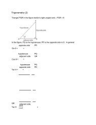
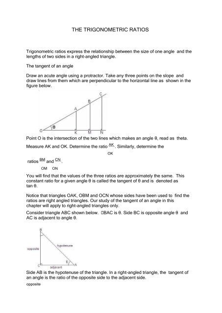
THE TRIGONOMETRIC RATIOS
Trigonometric ratios express the relationship between the size of one angle and the
lengths of two sides in a right-angled triangle.
The tangent of an angle
Draw an acute angle using a protractor. Take any three points on the slope and
draw lines from them which are perpendicular to the horizontal line as shown in the
figure below.
Point O is the intersection of the two lines which makes an angle θ, read as theta.
Measure AK and OK. Determine the ratio AK . Similarly, determine the
ratios BM and CN .
OM
ON
You will find that the values of the three ratios are approximately the same. This
constant ratio for a given angle θ is called the tangent of θ and is denoted as
tan θ.
Notice that triangles OAK, OBM and OCN whose sides have been used to find the
ratios are right angled triangles. Our study of the tangent of an angle in this
chapter will apply to right-angled triangles only.
Consider triangle ABC shown below.
AC is adjacent to angle θ.
OK
BAC is θ. Side BC is opposite angle θ and
Side AB is the hypotenuse of the triangle. In a right-angled triangle, the tangent of
an angle is the ratio of the opposite side to the adjacent side.
opposite

Thus, tan θ .
adjacent
Exercise
1. Name the sides which are opposite and adjacent to the angle marked θ in each

When the angles are known, we use the table of tangents to find the ratios of the
opposite to the adjacent sides. Angles in the table of tangents are expressed in
degrees and points of degrees. They are also given in minutes.
There are 60 minutes (60’) in 1 degree (1 0 ). Thus, 60’ is equivalent to 1 0 . There are
three major groups of columns in the table of tangents as in table 12.1.
1. The column headed θ gives angles in degrees.
2. The next 10 columns headed 0.0 0 to 0.9 0 or 0’ to 54’ give the tangents of angles.
Angles increase in steps of 6’ or one-tenth of a degree which is 0.1 0 .
3. The last five columns headed 1’ to 5’ are called differences and indicate
hundredths of degrees.
Example
Find tan 12.8 0 .
Solution
To find tan 12.8 0 , proceed as follows:
In the column headed θ, look for the row headed 12. Move along this row until you
reach the column headed 0.8. The number at the intersection is 0.2272. Therefore,
tan 12.8 0 = 0.2272. Note: 12.8 0 = 12 0 48’
In order to find tan 12 0 48’ read the number where the row headed 12 0 meets with the
column headed 48’.
Example
Find tan 12 0 45’
Tan 12 0 45’ cannot be read directly from the table because there is no column for 45’.
12 0 45’ lies between 12 0 42’ and 12 0 48’ both of whose tangents can be directly read
from the tables.
Since 12 0 45’ is 3’ more than 12 0 42’, the difference between their tangents is the
number at the intersection of the row headed 12 0 and the column headed 3’, that is,
0.0009. This difference is then added to the value of tan 12 0 42’. Thus, tan12 0 45’ = tan
(12 0 42’ + 3’)
= 0.2263
= 0.2254 + 0.0009
Note: 12 0 45’ is also 3’ less than 12 0 48’.
The corresponding difference in their tangents is also 0.0009. This difference is
subtracted from the value of tan 12 0 48’.
Thus, tan12 0 45’ = tan 12 0 48’ – tan 3’

Exercise
= 0.2272 – 0.0009
= 0.2263
Use tables to find the tangents of the following angles:
1. 18 0 2. 80 0
3. 37 0 4. 5 0
5. 15.3 0 6. 44.9 0
7. 54.2 0 8. 7 0 15’
9. 63 0 50’ 10. 72 0 35’
11. 88 0 48’ 12. 20 0 58’
Using tangents in calculations
Example
Find length AB in triangle OAB
Solution
Tan 400 =
AB AB OB
15
AB = 15 tan 40 0
= 15 × 0.8391 (from the tables) = 12.6 cm.
Example
Find length PQ in triangle PQR.

Solution
Tan 70 0 21’ = 45
PQ
Hence, PQ = 45
= 16.07 cm.
=
45
tan 70 0 21 '
2 .800
Example
Find the size of angle θ in the figure below.
Solution
Tan θ = 3.5 = 0.4605
7.6
We need to find an angle, θ, whose tangent is 0.4605. In this case, the process of
finding the tangent of an angle is reversed. From the table of tangents, locate the
number 0.4605 or if it is missing, locate the nearest number smaller than it. The
closest smaller tangent to 0.4605 is 0.4599, the tangent of 24 0 42’. The difference
between 0.4605 and 0.4599 is 0.0006. Look for 6 (or the closest number) in the

difference columns along the row headed 24. The number closest to 6 is 7 in the
column headed 2’. Thus, the angle whose tangent is 0.4605, is 2’ more than 24 0 42’.
Therefore, θ = 24 0 42’ + 2’
= 24 0 44’
Exercise
1. Use tangents to find the lengths of the sides marked x in each of the following

its angles.
Applications of tangents Elevation and
Depression
(alternate angles).
Example
A boy, 120 cm tall, is standing 50 m from a flag post on a level ground. He finds that
the angle of elevation to the top of the flag post is 15 0 . Calculate the height of the
flag post.
Solution

= 13.4 m.
Tan 15 0 = BC (see diagram below)
50
Therefore, BC = 50 tan 15 0
= 50 × 0.2679
This is the height of the flag post above the boy’s height of 1.2 m. Therefore, the
height of the flag post is 13.4 + 1.2 = 14.6 m.
Example
A girl lying at the top of a cliff, 120 m high sees two rocks whose angles of depression
are 10 0 and 30 0 . If the rocks are in line with the foot of the cliff, find the distance
between the rocks.
In MBF, tan 10 0 = 120

= 120 = 681 m. tan100 0.1763
FB Therefore, FB = 120
The distance between the rocks is
m.
AB = FB – FA = 681 – 208 m = 473
Alternatively, in MFA, AMF = 60 0 .
Thus tan 60 0 = AF = AF
MF 120
Therefore, AF = 120 × 1.132 = 208 m.
And in FMB, BMF = 80 0 . Thus, tan 80 0 = FB
Therefore, FB = MF tan 80 0 = 120 × 5.671 = 681 m. AB = FB –
AF = 681 – 208 = 473 m.
Exercise
1. An angle of elevation of P from Q is 62 0 . What is the angle of depression of Q
from P?
MF
2. What is the angle of elevation of the top of a building, 30 m tall, from a point on
the ground 80 m away?
3. A ladder leans against a vertical wall making an angle of 15 0 with the wall. If its
foot is 4 m from the wall, calculate the height above the ground of the top of the
ladder.
4. A vertical tower, 40 m tall, casts a shadow on a level ground. Calculate the
angle the rays of the sun make with the ground.
5. The angle of elevation to the top of a tree from a point on the ground 70 m
from its foot is 18 0 . Calculate the height of the tree.
6. Calculate the angles of a rhombus whose diagonals are 14 cm and 8 cm.
7. P is 15 km north of Q and R is 26 km west of P. Calculate the bearing of R from
Q.
8. From the top of a rock, a boy sees a pawpaw tree 30 m away. He measures the
angle of elevation of the top of the tree as 15 0 and the angle of depression at the
bottom as 4 0 . Calculate the height of the pawpaw tree.

9. Two boys standing on opposite sides of a tree 24 m tall, measure the angles of
elevation of its top as 36 0 and 23 0 . Calculate the distance between the two
boys.
10. A tree that is 20 m from a busy path is being cut down. The angle of elevation
of the top of the tree from the middle of the path is 50 0 . Is it safe for the tree to
fall in the direction of the path?
11. How far from the base of a 25 m cliff must a ship be so the angle of elevation
of the top of the cliff from the ship is to be 7 0 ?
12. The angle of elevation of the top of a building is 70 0 from a point on the ground
50 m away.
(a)
How high is the building?
(b) What would be the angle of elevation of the top of the building from a
point on the ground 25 m away?
13. The angle of depression of a crossroads from an aero plane flying at 400 m is
20 0 .
(a)
(b)
What is the horizontal distance of the plane from the crossroads?
What would the angle of depression have been if the plane had been
flying at 600 m at the same horizontal distance away?
14. The angle of elevation of the top of a chimney on a house from a point on the
ground 50 m away is 22 0 .
(a)
(b)
How high above the ground is the top of the chimney?
If the angle of elevation of the roof of the house from the same point is
20 0 , how tall is the house? (c) How tall is the chimney?
15. The angle of depression of a house from the top of a 175 m hill is 75 0 . (a)
How far is the hill from the house, horizontally?
(b) If the angle of depression of a church from the top of the hill is 62 0 ,
How far is the hill from the church, horizontally?
(c)
Assuming that the hill, house and church are all in the same straight line,
how far is it from the house to the church?
16. (a) The angle of elevation of the top of a cliff from a ship at sea level is
12.3 0 . If the ship is 2.3 km out to sea find the height of the cliff.
(b) A 50 m lighthouse stands on the top of the cliff. Find the angle of
depression of the ship from the top of this lighthouse.
The sine of an angle
We have seen that for any right-angled triangle ABC, the ratio of the opposite side to
the adjacent side is a constant fro a given angle, θ.

Similarly, the ratio of the opposite to the hypotenuse is a constant for any given
angle, θ. This constant is called the sine of angle θ, abbreviated as sin θ and read as
sine theta.
sin θ = .
opposite Thus,
hypotenuse
The table of sine
The table of sines is read in the same way as the table of tangents. For example,
sin 24 0 = 0.4067 and sin 43 0 46’ = 0.6909 + 0.0009 = 0.6918 Exercise
1. Write down the sines of each of the following angles:
(a) 13 0 (b) 76 0
(c) 44.3 0 (d) 50 0 24’
(e) 32 0 19’ (f) 18 0 16’ 2.
Write down the angles whose sines are:
(a) 0.8746 (b) 0.3272
(c) 0.8398 (d) 0.3555
(e) 0.6000 (f) 0.9927
Applications of sines
Example
Find the length of PR in the following diagram.

Solution
Sin 38 0 = PR = PR
RQ 80
Thus, PR = 80 sin 38 0
= 80 × 0.6157 = 49.3 cm.
Example
Find the size of angle θ in the following diagram.
Exercise
Solution
Sin θ = = 0.4615
θ = 27 0 29 ’
1. Find the length of the side marked x in each of the following right-angled
triangles:
(a)
(b)

2. Find the size of the angle marked θ in each of the following right-angled
triangles:

( a ) ( b)
( c) ( d)
3. In triangle ABC below, find the length of BC.
4. An isosceles triangle with its base 18 cm long, has each of the identical angles
as 43 0 . Find the lengths of the identical sides.
5. In the figure below, triangles ABC and ABD are right-angled.

Find: (a) BAD, (b) the length of BC.
6. Find the base length of an isosceles triangle whose vertex angle is 50 0 and the
equal sides are 10 cm long.
7. An isosceles triangle has a base of 6 cm and the equal sides are each 8
cm long. Find the angles of the triangle and its height.
8. Find the angle subtended at the centre of a circle of radius 5 cm by a chord of
length 3 cm.
The cosine of an angle
In any right-angled triangle, the ratio of the adjacent side to the hypotenuse is a
constant for any given angle, θ. This constant ratio is called the cosine of angle θ,
abbreviated as cos θ.
Thus, cos θ = .
a d ja ce nt
hyp o te nuse
The table of cosines
You will have noticed that the sines and tangents of angles increase as the angles
increase. In the table of cosines, the cosine of angles decrease as the angles
increase.
The cosines of angles are read in the same way as the sines except that the values
in the columns of differences of the cosines are subtracted instead of being added.
Example
(a) Find cos 35 0 22’.
(b) Find the angle whose cosine is 0.6890
Solutions
(a) From the tables, cos 35 0 22’ can be found by getting cos 35 0 18’

Cos 28 0 14΄ = AB = 40 AC AC
Cos 35 0 18’ = 0.8161
35 0 22’ – 35 0 18’ = 4’
Therefore, cos 35 0 22’ = 0.816 – 0.0007 = 0.8154
(b) From the tables, 0.6890 lies between 0.6664 and 0.6896 in the row headed 46.
0.6896 is 0.0006 more than 0.6890. We look for 6 or a number nearest to 6 in
the differences column on the row headed 46 0 . The number 6 is in the column
3’. The angle whose cosine is 0.6890 is 46 0 24’ + 3’ = 46 0 27’. Exercise
1. Find the cosine of each of the following angles:
(a) 23 0 (b) 48 0 17’
(c) 67 0 9’ (d) 83 0 34’
(e) 42.6 0 (f) 15.7 0
2. Use tables to find the angles whose cosine are: (a)
0.2554 (b) 0.0870
(c) 0.8895 (d) 0.5978
(e) 0.4970 (f) 0.9998
Applications of cosines
Example
Find AC in the following diagram.
Solution
AC = 40 = 40 = 45.4 m. cos28014 0.8810

Example
Find the size of angle θ in the following diagram.
Exercise
Solution
Cos θ = = 0.5385 θ
= 57 0 25 ΄ (from tables)
1. Find the lengths of the sides marked x in the following right-angled triangles:
(a) (b)

2. Find the value of θ in each of the following right-angled triangles:
(a) (b)
3. A diagonal of a rectangle is 20 m long and makes an angle of 40 0 with one of
the sides. Calculate the lengths of the sides of the rectangle.
4. A rectangle 12 cm wide has a diagonal of 20 cm. Calculate the acute angle
between the diagonals.

5. A ladder 8 m long is leaning against a vertical wall, with its foot 2 m from the
wall. Calculate the angle the ladder makes with the floor.
6. A chord of a circle 13 cm long subtends an angle of 118 0 at the centre. Find the
radius of the circle.
7. A girl starts from village P, walks 300 m on a bearing of 038 0 to village Q, and
then walks 60 m on a bearing of 073 0 to R. Find how far east R is from P.
8. An isosceles triangle ABC is such that AB = BC = 16.5 cm, and ABC = 80 0 24΄.
Find the length of its altitude.
Tangents, sines and cosines
Consider a right-angled triangle PQR.
In the diagram above, sin θ = QR and cos θ = PR .
PQ
PQ
=
sin θ
QR ÷ PR = QR × PQ = QR Therefore,
cos θ PQ PQ PQ PR
PR
Also, tan θ = QR .
PR
Therefore,
tanθ
Example
A metallic pipe 12 m long is leaning against a vertical wall, with its foot 3 m from the
wall.
(a)
Find the angle the pipe makes with the horizontal.

(b)
Find the height of the wall where the pipe reaches.
Solution
Let the angle be θ and the height be h.
( a ) cos θ = = 0.25
Therefore, θ = 75 0 31 ΄
( b ) sin 75 0 h
31 ΄ =
12
That is, h = 12 sin 75 0 31΄ = 12 × 0.9682 = 11.6 m.
The ratios of sine, cosine and tangent are best remembered by the acronym
SOHCAHTOA.
Where, SOH means, Sine =
CAH means, Cosine =
means. Tangent = .
Hypotenuse
Opposite TOA
Adjacent
Opposite
Hypotenuse Adjacent
Example
Find without using tables, the value of sin θ and tan θ, if cos θ =
and θ is an acute
angle.

Solution
adjacent
Cos θ = hypotenuse
.
Draw following diagram.
ABC and indicate the sides as in
the AB = 4 units and AC = 5 units. Using Pythagoras’ theorem,
BC 2 = AC 2 – AB 2
= 5 2 – 4 2
= 9
BC = 3
Sin θ = BC 3 and tan θ = BC 3
AC 5 AB 4
Also, tan θ = = ÷ = × = .
Exercise
1. Given that tan x = , find cos x and sin x.
2. Given that cos x = , find sin x and tan x. 3.
Given that sin x = , find cos x and tan x.
4. Given that tan x = , find cos x and sin x.
5. If tan x =
5 cosx sinx
, evaluate
12 sinx
cosx

6. The shadow of a building, on a horizontal ground, is twice as long as its height.
If its height is 25 m, calculate the angle of elevation to the sun from the ground.
7. In the figure below, calculate the lengths of lines: (a) AD (b) AB
(c)
BC
STATISTICS
Statistics is that branch of mathematics which is concerned with the collection,
organization, interpretation, presentation and analysis of numerical data. To a
statistician, any information collected is called data. When data has not been ordered
in any specific way after collection, it is called raw data.
Representation of data
Frequency tables (distributions)
The frequency of an event is the number of times that the event occurs. While
counting the scores, a tally mark, /, is made for every count and the fifth stroke
crosses over the other four to have . Example
Forty people were asked to judge which of five paintings, labeled A, B, C, D and E,
was the best. The results are given below.
B C B B D A E A
C C A A B D E A B D B B B
C A D
E B C A A C D B
C C A D B B D A
If a prize was given for the picture with the most votes, which picture won?

Solution
First we put the data into a frequency distribution (frequency table). This is a table
which gives each data item together with the number of times they occur.
Painting
Tallies Frequency
A
B
C
D
E
Total
10
12
8
7
3
40
Painting B, with twelve votes, wins the prize.
The above data may be displayed in various ways.
Bar chart:
Bar charts or graphs can be used to make quick comparison of data. They are either
horizontal or vertical, jointed or disjointed. The height or the length of the bar
represents the frequency and its width is not significant.
The bar graph for the above data can thus be drawn as follows.

Pie Chart:
In a pie chart, each number is represented by the area of a sector of a circle. The
frequency is proportional to the angle of the sector.
The forty votes are represented by 360 0 (a full turn); thus one vote is represented by
360 0 40 = 9 0 .
Frequency
Angle
A 10 10 9 = 90 0
B 12 12 9 = 108 0
C 8 8 9 = 72 0
D 7 7 9 = 63 0
E 3 3 9 = 27 0
Line graphs

A line graph is used to show how things change over a period of time. For example: A
student obtained the following marks in six mathematics weekly tests. Draw a line
graph to represent this information.
Test 1 2 3 4 5 6
marks 60 65 80 75 85 90
To draw the line graph, mark the test numbers on the horizontal axis and the marks
on the vertical axis. Plot the ordered pairs on the graph with dots as shown in the
figure below. To obtain the line graph, join the dots with straight lines.
Measures of central tendency
These are values about which the distribution of data in a particular se may be
approximately balanced. The common ones include the mean, median and mode.
The mean ( x)
The mean is the value obtained when the total sum of the values of the members in a
list or distribution is divided by the total frequency.
Example
The masses (in kilograms) of nine students are 42, 47, 52, 57, 62, 67, 72, 77 and 82.
Calculate their mean mass.
Solution
Add all the masses together and divide by 9.

The sum of the masses is 558 kg. The total
number of students is 9.
The mean mass is
= 62 kg.
Example
Find the mean of the following frequency distribution.
Solution
x 1 2 3 4 5 6
f 2 4 1 3 3 3
To calculate the mean of the above data the following steps are followed.
• Multiply each frequency (f) by its corresponding value (x) to obtain the product
(f.x)
• Find the sum of the products, (f.x), and then divide this sum by the sum of the
( f . x )
frequencies (f) to obtain the mean, i.e. x f
x f f.x
1 2 2
2 4 8
3 1 3
4 3 12
5 3 15
6 3 18
f=16
f.x = 58
The mean, x = 3.625.
In statistics, the symbol (sigma) is used to mean the sum of. Thus, the sum of the
frequencies (f) is written as f and the sum of the products (f.x) is written as fx.
The median
Median is the middle value of a given set of data when all the entries are arranged in
order of size. It is the point at which exactly half of the data are above and half are
below.

In ungrouped data, if the total number of members in a list is odd, the median position
is a whole number given by (n 1) th member of the group. This formula gives the
position at which the median is found in ranked data. To get the median, we go back
to the ranked data and look for the value or entry at the position obtained from the
calculation. When the position is not a whole number, we get the average of the
values just before and just after the one obtained through the computation.
Example
Find the median of each of the following lists of numbers.
(a) 1, 7, 1, 6, 2, 5, 2, 5, 2, 5, 3, 5, 3, 4, 4.
(b) 29, 12, 25, 14, 18, 21, 18, 20, 19, 20.
Solutions
(a)
Rearranging the numbers in order of size, we have:
1, 1, 2, 2, 2, 3, 3, 4, 4, 5, 5, 5, 5, 6, 7
The number of members (n) is 15. The median is the (15 1)th member. That is
the 8 th member. From the ordered list, the 8 th member is 4. The median is 4.
(b)
Rearranging the numbers in order of size, we get:
12, 14, 18, 18, 19, 20, 20, 21, 25, 29
The number of members (n) is 10. The median position is given by
(10 1)= 11 = 5.5
This means that the median value falls between the 5 th and 6 th members in the
ordered data, and its value is their average.
The 5 th and 6 th members are 19 and 20 respectively. Therefore, the median is
= 19.5.
The median does not need to be among the numbers in the set of data.
The median of an ungrouped frequency distribution
In order to find the median using cumulative frequencies or the number of members
that lie above or below a particular value in a set of data, we must calculate the first
value with a cumulative frequency greater than or equal to the median.
Example
Find the median of the following distribution.
x 2 3 4 5 6 7 8
f 4 8 20 20 2 2 4

Solution
The total frequency, f = 60. The median position is (60 1) = 30.5. This means the
median value lies between the 30 th and 31 st values in the ordered data and its value
is their mean.
In order to get the 30 th and 31 st values, we need to make a cumulative frequency
table as shown below.
x Freq.
Cumulative frequency
(f) (cf)
2 4 4
3 8 12
4 20 32
5 20 52
6 2 54
7 2 56
8 4 60
The cumulative frequency is obtained by adding all the frequencies below and up to
and including the particular value. From the table, we can see that the cumulative
frequency corresponding to x = 8 is 60. This is the total number of observations in the
distribution. From the cumulative frequency it can be seen that the 30 th member is 4
and the 31 st member is also 4. Therefore, the median is = 4.
The mode.
The mode of a distribution is the most frequently occurring value. In a frequency
distribution, the mode is the value with the highest frequency.
Example
Find the mode of the following set of numbers. 2, 4,
4, 5, 7, 7, 7.
Solution
The mode is 7 as this appears three times.
Example
Find the mode of the following frequency distribution.

(a)
x 3 4 5 6 7
(b)
f 1 3 8 10 4
x 12 13 14 15 16
f 6 9 9 3 5
Solutions
(a) The mode is 6.
(b) The mode is 13 and 14 as these have the highest frequency.
Exercise
1. Find the mode, mean and median of the following sets of numbers
(a) 3, 5, 6, 8, 9, 9, 9
(b) 10, 10, 10, 20, 30, 30, 30, 30. (c)
7, 1, 3, 5, 2, 9, 1.
2. The mean of 4 numbers is 8. If three of the numbers are 4, 5 and 10, find the
fourth number.
3. The total of the heights of twenty-six girls was 41.86 m. Find the mean height of
the girls.
4. In a year, a student scored the following marks in tests and examinations.
Term Test 1 Test 2 Test 3 Exams
1 75 51 62 49
2 54 45 64 74
3 80 60 67 39
Calculate the student’s mean score.
5. The number of litres of milk delivered to 50 houses on one morning is shown
below.
No. of litres 1 2 3 4 5 6

No. of
house
10 14 18 4 2 2
Calculate the mean number of litres delivered per house.
6. The table below shows the marks scored by students in a test.
Mark 0 1 2 3 4 5
No. of
students
2 6 15 8 10 2
Calculate the mean and median mark.
7. The lengths, in centimeters, of 10 nails are: 3.01, 2.96, 3.04, 2.98, 3.00, 2.97,
2.99, 3.02, 3.03, and 2.94. Find the median length of the nails.
8. The number of goals scored in super league matches is shown in the table
below.
Goals frequency
0 10
1 20
2 10
3 6
4 9
4 8
Calculate the mean and median number of goals scored. State the modal
number of goals scored.
9. A company’s costs are split into the following categories.
Wages 45%
Rates 15%
Materials 30%
Transport 10%
Show this information in a pie chart.

10. A group of fifty year olds were asked how much television they had watched on
a particular evening. Their answers, to the nearest hour, are shown below.
(a)
1 3 0 3 1 4 5 4 3 2
0 4 6 2 2 2 3 2 2 7
3 1 0 2 3 3 0 1 7 2
5 4 2 1 1 3 4 2 4 4
0 0 1 2 1 3 1 2 7 2
Set up a frequency distribution to represent this information.
(b) Draw a bar chart to show the above data. (c) State the modal time.
11. Various types of large white loaves are delivered to a supermarket. The number
of each type delivered on a particular day is shown below.
Thin sliced 45
Medium sliced 84
Thick sliced 15
Uncut 36
(a) In a pie chart, what angle would represent 1 loaf? (b) Display the above
information in a pie chart.
12. The bar chart below shows the number of pages per day in the New Vision
news paper for 20 days during a certain month.
(a)
(b)
State the modal number of pages.
Calculate the mean and median number of pages.
13. The table below shows the number of letters collected by a school from the post
office in the first six weeks of the term.
Week 1 2 3 4 5 6
No. of 80 110 120 160 110 120
letters
Show this information in a:

(i)
(ii)
bar graph,
line graph.
14. The table below shows the production of eggs by 200 hens in 7 days.
Day 1 2 3 4 5 6 7
No. of
trays
1 2 2 3 4 5 6
(a) Draw:
(i) a bar
graph to show this data, (ii) a line graph
to represent the information.
(b) A tray of eggs costs sh.3, 000. How much money was collected in the 7
days?
15. The table below shows the number of trays of eggs supplied to a hotel by two
farmers.
Days 1 2 3 4 5 6 7
Farmer
A
8 10 12 15 12 11 8
Farmer 10 12 11 12 14 16 18
B
Draw line graphs to represent this data.
16. After a national examination at the end of secondary school education, students
from six schools were selected to attend university as follows:
School A B C D E F
No. of
students
60 45 30 90 15 60
Show this information on a pie chart.
17. A farmer grows five types of crops in a 24-hectare farm. The pie chart below
shows how the crops are distributed on the farm.

(a)
Calculate the area, in hectares, that each type of crop occupies. (b)
Show this information on a bar graph.
18. The mean mass of three men is 62 kg. Four women weigh 61 kg, 66 kg, 65 kg
and 69 kg. Find the mean mass of the 7 people.
19. Four farmers have the following number of animals: 25, 23, x and 2x. If the
mean number of animals per farmer is 24, find the value of x.
20. A car traveled at a speed of 80 km/h for 30 minutes, 70 km/h for 40 minutes and
90 km/h for 20 minutes. What was the average speed for the whole journey?
21. The average mass of 12 people in a lift is 68 kg. The maximum mass allowed in
the lift is 750 kg.
(a)
(b)
By how many kilograms was the lift overloaded?
How many people should come out of the lift to allow it to move?
22. The table below shows the ages of 11 girls in a soccer team.
Age in
years
15 16 17 18 19
Frequency 2 4 2 1 2
Find the:
(a) modal age,
(b) median age, (c) mean age.
Statistics(2)
(a) Statistics is that branch of mathematics which is concerned with the collection,
organization, interpretation, presentation and analysis of numerical data. To a
statistician, any information collected is called data. When data has not been
ordered in any specific way after collection, it is called raw data.
(b) Discrete data. This is a type of data which can take only exact or integral
values. For example, the number of cars passing a check point in 30 minutes;
the number of students served in the dinning hall in five minutes, etc.
(c) Continuous data. This is data which cannot take exact or integral values, but
can be given only within a certain range or measured to a certain degree of
accuracy. For example, the heights of students in a school; the time taken by
each of a class of students to perform a task, etc.

Methods of presentation of data
Pie Chart.
In a pie chart, each number is represented by the area of a sector of a circle.
The frequency is proportional to the angle of the sector.
Example
The table below shows the number of cars of different colors in a car park. Draw a
pie chart to represent this information.
Color Green Blue Yellow Others
Number 10 14 20 16
The angles of the sectors are calculated as follows:
The total number of cars = 10 + 14 + 20 + 16 = 60
Angle representing green cars = 360 0 = 60 0
Angle representing blue cars = 360 0 = 84 0
Angle representing yellow cars =
360 0 = 120 0 Angle
representing other cars = 360 0 = 96 0 .
Frequency Distributions

(a) Discrete data:
To illustrate data more concisely we count the number of times each value
occurs and form a frequency distribution. For example, the following data
gives the number of blind students in 10 randomly chosen classes in certain
school. 0, 2, 1, 4, 2, 3, 2, 1, 4, 5. this information can be presented as follows:
Number of students Frequency
0 1
1 2
2 3
3 1
4 2
5 1
Total 10
(b) Continuous data:
In connection with large sets of data, a good overall picture and sufficient
information can often be conveyed by grouping the data into a number of
classes (intervals).
General rules for grouping data:
(i) Determine the largest and smallest numbers in the raw data and find the
difference between them.
(ii) Divide this difference into appropriate number of class intervals having the
same size – the number of intervals usually taken is between 5 and 20
depending on the size of the data (but preferably 7 to 10 for medium data).
If this is not feasible use class intervals of different sizes or open class
intervals.
(iii) Determine the number of observations falling into each class interval i.e.
find the class frequencies. This is best done by using tallies. (iv)
Display the results in the form of a table.
Example
Construct a distribution of the following data on the length of time (in minutes) it
took 80 persons to complete a certain task.

23 24 18 14 20 24 24 26 23 21
16 15 19 20 22 14 13 20 19 27
29 22 38 28 34 32 23 19 21 31
16 28 19 18 12 27 15 21 25 16
30 17 22 29 29 18 25 20 16 11
17 12 15 24 25 21 22 17 18 15
21 20 23 18 17 15 16 26 23 22
11 16 18 20 23 19 17 15 20 10
Solution
Since the smallest value is 10 and the highest is 38, we might choose the three
classes 10-19, 20-29, and 30-39; we might choose the six classes: 10-14, 15-19,
20-24, 25-29, 30-34, and 35-39; to mention a few possibilities. Note that in each
case the class intervals accommodate all of the data, they do not overlap, and
they are all of the same class size. Taking the second classification, we now tally
the 80 observations and get the results shown in the following table.
Minute Tally Frequency
10 – 14 8
15 – 19 28
20 – 24 27
25 – 29 12
30 - 34 4 35 - 39
1 total 80
The numbers given in the right hand column of this table, which show how many
items fall into each class, are called class frequencies. The smallest and largest
values that can go into any given class are referred to as its class limits, and in
our example they are: 10, 14, 15, 19, 20,…., 34, 35, and 39. More specifically, 10,
15, 20, … and 35 are called the lower class limits, and 14, 19, 24, 29, 34 and 39
are called the upper class limits.
The lengths of time which we grouped in our example were all given to the
nearest minute, so that the first class actually covers the interval from 9.5 minutes
to 14.5 minutes, the second class covers the interval from 14.5 to 19.5, and so
forth. These numbers are referred t as class boundaries or the “real” class limits.
Class marks are simply the midpoints of the classes, and they are obtained by the
formula:

lowerclasslim upperclasslim
Class mark =
Or
upperclassboundary lowerclassboundary
2
2
A class interval (width or size) is the length of a class, or the range of values it can
contain and is given by the difference between its class boundaries. If the classes
are of equal length, their common class width is also given by the difference
between any two successive class marks.
Note that the class widths are not given by the differences between the respective
class limits.
Cumulative frequency
Cumulative frequency is the total frequency up to a given point.
Example
Convert the distribution above into a cumulative frequency distribution.
Solution
Since none of the values is less than 10, 8 are less than 15, 8+28 = 36 are less
than 20, 8+28+27 = 63 are less than 25, … the results are as shown in the
following table.
Minutes Cumulative freq.
Less than 10 0
Less than 15 8
Less than 20 36
Less than 25 63
Less than 30 75
Less than 35 79
Less than 40 80
Histograms

A histogram is constructed by representing the measurements or observations that
are grouped on a horizontal scale, the class frequencies on a vertical scale, and
drawing rectangles whose bases equal the class intervals (widths) and whose
heights are determined by the corresponding class frequencies. The markings on the
horizontal scale are class boundaries.
When class widths are not all equal, the class frequencies are represented by the
areas of the rectangles instead of their heights. The vertical axis is not labeled
frequency but frequency density. frequency
Frequency density =
classwidth
Because the area of the bar represents frequency, the height must be adjusted to
correspond with the area of the bar.
Histograms can be used to represent both discrete and continuous data, but their
main purpose is for use with continuous data.
Example
Draw a histogram for the data given below.
Time Tally
Frequency
(Minutes)
10 – 14 8
15 – 19 28
20 – 24 27
25 – 29 12
30 - 34 4
35 - 39 1
Solution
total 80

Time
(Minutes)
Class
boundaries
Frequency
10 – 14 9.5 – 14.5 8
15 – 19 14.5 – 19.5 28
20 – 24 19.5 – 24.5 27
25 – 29 24.5 – 29.5 12
30 - 34 29.5 – 34.5 4
35 - 39 34.5 – 39.5 1
total 80
Note that all classes have equal width and therefore, we plot frequency against class
boundaries.
Example
The ages of 120 people who traveled by air on Christmas day were recorded
and are shown in the frequency table.
Age (yrs)
Frequency
– 10 18
– 20 46
– 30 35
– 40 13
Solution
- 50 8
The notation ‘- 10’ means ‘0 < age
10’ and similarly ‘– 20’ means
‘10 < age 20’. The class boundaries are 0, 10, 20, 30, 40 and 50.
The histogram is then drawn as shown in the diagram below (see next page).

Frequency polygons.
In these, class frequencies (or frequency densities in case of a distribution with
unequal class width) are plotted against the class marks and the successive points
are connected by means of straight lines. Classes with zero frequencies are added at
both ends of the distribution so as to obtain a closed polygon.
Example
Draw a frequency polygon for the data below.
Weight (kg) Class marks Frequency
30 – 40 35 5
40 – 50 45 7
50 – 60 55 10
60 – 70 65 5
70 - 80 75 3
Solution:

Weight (kg)
A frequency polygon can also be formed by joining the mid-points of the tops of the
rectangles in a histogram by straight lines. This is known as ‘superimposing’ a
frequency polygon on a histogram (see diagram below).
Cumulative frequency curve (Ogive)

Cumulative frequency is the total frequency up to a given point. A cumulative
frequency curve is obtained by plotting cumulative frequency against the upper class
boundaries and the points connected by means of a smooth curve. A class with zero
frequency is added at the beginning of the distribution so that the resulting curve
starts from the ‘origin’.
Example
The marks obtained by 80 students in an examination are shown below.
Mark frequency Cum. frequency Upper class boundaries
- 0 0 0 0.5
1 – 10 3 3 10.5
11 – 20 5 8 20.5
21 – 30 5 13 30.5
31 – 40 9 22 40.5
41 – 50 11 33 50.5
51 – 60 15 48 60.5
61 – 70 14 62 70.5
71 – 80 8 70 80.5
81 – 90 6 76 90.5
91 -
100
4 80 100.5
The corresponding Ogive is then plotted as shown in the following diagram.

Marks
Measures of central tendency
The measures of central tendency are the mean, median and mode. These are
Values about which the distribution of a set of data is considered to be roughly
balanced.
The mean
The mean is the value obtained when then the total sum of the values of the
members in a list or distribution is divided by the total frequency. The mean can be
obtained for grouped or ungrouped data.
Example
On a certain day, nine students received, respectively, 1, 3, 2, 0, 1, 5, 2, 1and 3
pieces of mail. Find the mean.
Solution
The total number of pieces of mail which these students received is
1+3+2+0+1+5+2+1+3 = 18, so that the mean number per student is
Mean = 2

Suppose xi represents the number whose mean is to be calculated (x1, x2, x3, x4, …,
x
xn). In this set there are n values. So Mean = x 1 2
... x n orx
x , where x =
x1+x2+x3+…+xn. n n
is capital sigma, the Greek letter for S. The notation x stands for “the sum of the
x’s”.
If data is in the form of a frequency distribution, the mean is calculated using the
formula:
Mean =
x.f , where x.f means ‘the sum of the products’
f
i.e. (number
frequency) and f means ‘the sum of the frequencies’.
Example
The marks obtained by 100 students in a test were as follows:
Find the mean mark.
Mark (x) 0 1 2 3 4
Frequency (f) 4 19 25 29 23
Solution
Mean = = 2.48.
Mark (x)
Freq.
(f)
x.f
0 4 0
1 19 19
2 25 50
3 29 87
4 23 92
total 100 248
For grouped data, each class can be represented approximately by its mid-point
(class mark)
Example
The results of 24 students in a Mathematics test are given in the table.

Mark Freq. Mid-point(x) x.f
85 – 99 4 92 368
70 – 84 7 77 539
55 – 69 8 62 496
40 - 54 5 47 235
f=24 x.f= 1,638
Mean = = 68.25.
Example
The number of letters delivered to the 26 houses in a street was as follows:
Number of letters Number of houses (i.e. freq.)
0 – 2 10
3 – 4 8
5 – 7 5
8 - 12 3
Calculate an estimate of the mean number of letters delivered per house.
Using an assumed mean
When the number of members in a list is large, the above method of finding the mean
is quite ardous. From the data we can guess the expected value of the mean. This
expected value is called the assumed or working mean. The assumed mean is
approximately in the middle of the data. In a frequency distribution table, the modal
value provides the best assumed value. The assumed mean does not need to be one
of the values given.
Example
The table below shows the profit made by a trader in 100 days.
Profit in ‘000
Ush.
115 125 135 145 155 165
No. of days 8 18 30 26 12 6
Calculate the mean profit
Solution

To calculate the mean of the above data using an assumed mean, the following steps
should be followed.
Step 1: Choose an appropriate assumed mean (A) for the range of the values given.
Step 2: Find by how much each of the values (x) differs from this assumed mean
(A). These differences obtained are called deviations (d). Thus, d = x – A.
Step 3: Multiply each frequency (f) by its corresponding value of deviation (d) to
obtain the product (fd).
Step 4: Find the sum of the products, ∑(fd), and then divide this sum by the sum of
∑fd
the frequencies to obtain the mean of the deviations, ∑f
∑fd
Step 5: Find the mean by using the formula: x=A+
∑f
The table below is a summary of the calculations where the assumed mean is 135
(the modal value).
= 135 + ( ) = 135 + 3.4 = 138.40
The mea profit is sh. 138.40 ×1000 = sh. 138,400.
The Median
The median of a set of data is a number selected to represent the middle position
when the data are arranged in order of size. The middle position in an array of N data
items is the position numbered
. If N is odd, there is a data item at the middle
and we take this item as the median. If N is even, we take the average of the two
middle data items as median.

Example
The median of 18, 22, 30, 31, 44, 60 and 68 is 31 obtained as follows:
Since N = 7, position of the median is = 4 th data item.
Example
Find the median of the following numbers. 4, 4, 10, 3, 3, 6, 7, 4, 6, 7.
Solution
Arranging numbers in order of size, we have
3, 3, 4, 4, 4, 6, 6, 7, 7, 10.
Position of median:
= 5.5. So the median lies between the 5 th and 6 th data items
i.e. between 4 and 6. Hence, the median is = 5.
Example
The marks obtained by 100 students in a test were as follows.
Mark (x) 0 1 2 3 4
Frequency
(f)
4 19 25 29 23
Find the median mark.
Solution
The median is the number between the 50 th and 51 st numbers. By inspection, both
the 50 th and the 51 st numbers are 3. Therefore, the median = 3 marks.
It should be noted that, the formula
tells us its position.
is not a formula for the median; it simply
For grouped data, the median is given by the following formula:
Median = L b N2 fF mm 1 i .
Where, Lb = lower class boundary of the median class;

Fm-1= cumulative frequency of the class before the median class;
fm= frequency of the median class; i= class width of the median
class; N = total frequency.
Example
The table below shows the weights of 40 poles in kg.
Find the median weight.
Weight (kg) frequency Cumulative freq.
118 – 126 3 3
127 – 135 5 8
136 – 144 9 17
145 – 153 12 29
154 – 162 5 34
163 – 171 4 38
172 - 180 2 40
We find the median class first. Since
20, we look for where 20 is cumulated in the
cumulative frequency column. We note that at cumulative frequency of 17, we need 3
more to get 20. So 3 are found in the cumulative of 29. And so ‘145 – 153’ is the
median class.
Thus, Lb = 144.5; Fm-1= 17; fm = 12; i = 9.
Hence, median = 144.5+ 9
= 146.75 kg.
= 144.5 + 2.25
Median from an Ogive:
A cumulative frequency curve shows the median at the 50 th percentile of the
cumulative frequency.
For instance, in figure 5, N = 62 and the therefore the 31 st data item gives the median
which is obtained by drawing a horizontal line, from the cumulative frequency axis to
the curve, and then drawing the line down wards to the horizontal axis. From the
Ogive, the median mark is 49.

The mode
Another measure which is sometimes used to describe the “middle” of a set of data is
the mode. It is defined as the value which occurs with the highest frequency.
Example
Find the mode of the following numbers: 5, 4, 10, 3, 3, 4, 7, 4, 6, 5. The mode is 4.
(There are more 4’s than any other number).
For grouped data, the mode is estimated using the following formula.
Mode = l b +
d 1
d d
1
2
i
Where, lb = lower class boundary of the modal class (i.e. the class containing the
mode);
d1 = the difference between the frequency of the modal class and the
frequency of the class before it;
d2 = the difference between the frequency of the modal class and the
frequency of the class after it;

Example
i= class width of the modal class.
Find the mode of the following data.
Cass Frequency
20 – 22 3
23 – 25 6
26 – 28 12
29 – 31 9
32 - 34 2
Solution
The modal class is the class with the highest frequency or frequency density (in case
the classes have unequal widths).
Thus the modal class for this data is ’26 – 28’.
So lb = 25.5, d1 = 12 – 6 = 6, d2 = 12 – 9 = 3, i= 3.
Mode = 25.5 + 3 = 25.5 + = 27.5.
When a histogram is drawn, the mode is obtained by joining the ends of the highest
rectangle to the opposite ends of the rectangles next to it as shown in the figure
below.
Quartiles

These are values that divide the data into four equal parts. They are denoted by Q1,
Q2 and Q3. Q1 divides the data into ¼, Q2 into and Q3 into ¾. In other words, for
Q1, 25% of the values are below it, Q2 takes 50% and Q3 takes 75%.
Q1 is called the first (or lower) quartile, Q2 the second quartile (median) and Q3 the
third or upper quartile.
For ungrouped data, the position of Q1 is given by ¼(n+1)th value, while that of Q3 by
¾(n+1)th value. In each case n is the number of observations.
Example
(i) Find the lower and upper quartiles of the following set of numbers: 3, 12, 4, 6, 8, 5,
4.
Arranging the numbers in order of size, we have 3,
4, 4, 5, 6, 8, 12.
Position of Q1: ¼(7+1)th = 2 nd value.
Therefore, the lower quartile is 4.
Position of Q3: ¾(7+1)th = 6 th value.
Therefore, the upper quartile is 8.
For grouped data, the following formulae are used:
Q1 = L b
4
N Fq 1 3N Fq 1
i ; Q3= L b
4
i
f q
fq
Where,
Lb = lower class boundary of the quartile class;
Fq -1 = cumulative frequency of the class before the quartile class;
fq = frequency of that quartile class; i = class width of the quartile
class; N = the number of observations in the data.
Example
The table below shows the distribution of marks gained by a group of students in a
mathematics test marked out of 50.
Estimate the lower and upper quartiles.

Marks Frequency Cum. Freq.
1 – 10 15 15
11 – 20 20 35
21 – 30 32 67
31 – 40 26 93
41 - 50 7 100
Position of Q1 is ¼ 100 = 25 th observation. Using the cumulative frequency column,
the 25 th observation is located in the ‘11 – 20’ class. This is the lower quartile class.
So, Lb = 10.5, Fq-1 = 15, fq = 20, i = 20.5 – 10.5 = 10.
100 15
Therefore, Q1 = 10.5
4
20
10
= 10.5 + 5 = 15.5 marks.
Position of Q3: ¾ 100 = 75 th observation (mark). Using the cumulative frequency
column, the 75 th observation is located in the ‘31 – 40’ class.
So, Lb = 30.5, Fq-1 = 67, fq = 26, i = 40.5 – 30.5 = 10, N = 100.
Q3= 30.5 75 67 10
26
= 30.5 + 3.0769 = 33.5769
33.58 marks.
We define the inter-quartile range as: Q 3
Q 1, And
semi-interquartile range as: Q 3 Q 1
.
2
From the Ogive, the value at the 25 th percentile is the lower quartile, and that at the
75 th percentile is the upper quartile.

Example
Plot an Ogive for the above data and use it to estimate the semi-interquartile range.
Marks Frequency U.C.B Cum.
Freq.
0 0.5 0
1 – 10 15 10.5 15
11 – 20 20 20.5 35
21 – 30 32 30.5 67
31 – 40 26 40.5 93
41 -
50
7 50.5 100
Example
The following frequency distribution table gives the marks obtained by 500
candidates in an examination.
Mark frequency
1 ≤x< 10 15
10 ≤ x< 20 25

20 ≤ x < 30 39
30 ≤ x < 40 77
40 ≤x < 50 101
50 ≤ x < 60 84
60 ≤x < 70 61
70 ≤ x < 80 53
80 ≤ x < 90 22
90 ≤ x < 100 23
(a) Draw a cumulative frequency curve for the data.
(b) From your graph estimate:
(i) the median mark.
(ii) the pass mark, if 65% of the candidates passed.
(ii) the number of candidates who scored less than 45 marks.
Solution
(a) Construct a cumulative frequency table.
Upper
boundary
cf
10 15
20 40
30 79
40 156
50 257
60 341
70 402
80 455
90 477
100 500
Plot the cumulative frequency against the upper class boundaries. The figure below
shows the cumulative frequency curve.

(b) (i) The median mark is located ½ (500) th along the cumulative frequency
axis and the corresponding mark is 49.
(ii) If 65% passed, then 35% failed. From the graph, the pass mark is 42
(see the dotted line).
(iii) The number of candidates who scored less than 45 marks is 205.
Exercise
1. In an experiment, 50 people were asked to guess the weight of a mobile phone
in grams. The guesses were as follows:
47 39 21 30 42 35 44 36 19 52
23 32 66 29 5 40 33 11 44 22
27 58 38 37 48 63 23 40 53 24
47 22 44 33 13 59 33 49 57 30
17 45 38 33 25 40 51 56 28 64
Construct a frequency table using intervals 0 – 9, 10 – 19, 20 – 29, etc.
Hence draw a cumulative frequency curve and estimate:
(a) the median weight,
(b) the inter-quartile range,
2. In a competition, 30 children had to pick up as many paper clips as possible in
one minute using a pair of tweezers. The results were as follows:
3 17 8 11 26 23 18 28 33 38
12 38 22 50 5 35 39 30 31 43

27 34 9 25 39 14 27 16 33 49
Construct a frequency table using intervals of width 10, starting with 1 – 10.
From the frequency table, estimate the
(i) mean,
(ii) median of the distribution.
3. The mean weight of 8 boys is 55 kg and the mean weight of a group of girls is 52
kg. The mean weight of all the children is 53.2 kg. How many girls are there?
4. A group of 50 people were asked how many books they had read in the previous
year; the results are shown in the frequency table below. Calculate the mean
number of books read per person.
No of
books
0 1 2 3 4 5 6 7 8
Frequency 5 5 6 9 11 7 4 2 1
5. The following tables give the distribution of marks obtained by different classes
in various tests. For each table find the mean, median and mode.
(a)
Mark 0 1 2 3 4 5 6
Frequency 3 5 8 9 5 7 3
(b)
Mark 15 16 17 18 19 20
Frequency 1 3 7 1 5 3
Exercise
1. The table below shows the marks obtained, out of 50, by Form 4E students in a
Mathematics test.
Mark (x)
No. of students
(f)
1 – 10 9
11 – 20 10
21 – 30 11

31 – 40 8
41 - 50 7
Using an assumed mean, calculate the mean mark to the nearest whole number.
2. The marks obtained by 90 students in an end of term examination are given in
the table below.
Mark
(%)
No. of
students
1 – 10 4
11 – 20 5
21 – 30 10
31 – 40 11
41 – 50 12
51 – 60 15
61 – 70 10
71 – 80 9
81 – 90 8
91 -
6
100
Using 55.5 as the assumed mean, calculate the mean mark.
3. The heights of 50 army recruits were measured and tabulated as shown below.
Height (cm)
No. of
recruits
151 – 155 8
156 – 160 16
161 – 165 14
166 – 170 10
171 - 175 2
Using 160 cm as an assumed mean, calculate the mean height.
4. The table below shows the ages of students in a training college.

Age
18 ≤x<
20
20 ≤ x<
22
22 ≤ x <
24
24 ≤ x <
26
26 ≤x <
28
28 ≤ x <
30
30 ≤x <
32
32 ≤ x <
34
Frequency
7
10
33
21
14
13
10
4
Calculate the median age.
5. The frequency table below shows the marks scored by 45 students in a test.
(a)
(b)
Mark frequency
11 – 15 4
16 – 20 0
21 – 25 5
26 – 30 21
31 – 35 10
36 – 40 3
41 - 50 2
State the modal class.
Calculate the median mark.
6. The speeds of public service vehicles during a police check are shown in the
table below.

Speed
(km/h)
No. of
vehicles
31 – 40 5
41 – 50 10
51 – 60 15
61 – 70 30
71 – 80 55
81 – 90 70
(a)
(b)
91 -
15
100
Draw a cumulative frequency curve for this data.
Use your graph to estimate:
(i)
(ii)
(iii)
the median speed.
the lower and upper quartiles.
the percentage of vehicles traveling between 64km/h and
72 km/h.
7. The table below shows the distribution of marks of 81 candidates in a UCE
Mathematics examination.
Mark
No. of candidates
1 < x ≤10 1
10 < x ≤ 20 3
20 < x ≤ 30 9
30 < x ≤ 40 11
40 < x ≤ 50 14
50 < x ≤ 60 19
60 < x ≤ 70 11
70 < x ≤ 80 8
80 < x ≤ 90 4
90 < x ≤ 100 1
(a)
(b)
Draw a cumulative frequency curve to show the data.
Use your graph to estimate:

(i)
(ii)
(iii)
the median mark.
the upper quartile.
the number of candidates who scored less than 75 marks. (iv) The
pass mark, if 60% of the candidates passed.
8. The times taken by a group of students to solve a mathematical problem are
given below:
(a)
(b)
Time(min) 5 -
9
10 -
14
15 - 19 20 -
24
25 - 29 30 –
34
No. of
students
5 14 30 17 11 3
Draw a histogram for the data. Use it to estimate the modal time for solving a
problem.
Calculate the mean time of solving a problem.
9. The ages of 36 students are given below.
13 16 16 15 12 14 13 15 16
16 14 15 12 16 13 14 16 12
15 13 15 16 13 13 15 14 16
13 14 16 15 15 12 14 12 13
Make a frequency table and hence represent the age distribution of the students
on a frequency polygon.