563489578934
` Sec. 6–2 Power Spectral Density 427 t 1 =–T/2 =T/2-t 1 t 1 T 1 d T/2 3 dt 1 –T/2 0 T/2 2 d =–T/2-t 1 –T/2 t 1 =T/2 –T Figure 6–4 Region of integration for Eqs. (6–47) and (6–48). As seen in the figure, this is accomplished by covering the total area by using 2 when t 6 0 and 3 when t 0. Thus Eq. (6–47) becomes 0 t 1 = T/2 ƒ X T (f) ƒ 2 = c L L 2 3 (6–48) Now, assume that x(t) is stationary, so that R x (t 1 , t 1 t) = R x (t), and factor R x (t) outside the inner integral. Then 0 ƒ X T (f) ƒ 2 = R x (t)e -jvt ct 1 - L -T 0 T = (T + t)R x (t)e -jvt dt + (T - t)R x (t)e -jvt dt L L -T -T T t 1 = T/2-t + c R x (t 1 , t 1 + t)e -jvt dt 1 d dt L L 0 t 1 = -T/2- t ⎧ ⎪⎪⎪⎪⎪⎪⎪⎪⎪⎨⎪⎪⎪⎪⎪⎪⎪⎪⎪⎩ t 1 = -T/2 ⎧ ⎪⎪⎪⎪⎪⎪⎪⎪⎪⎨⎪⎪⎪⎪⎪⎪⎪⎪⎪⎩ T/2 T/2-t R x (t 1, t 1 + t)e -jvt dt 1 d dt T d dt + R(t)e -jvt ct 1` L 0 0 T/2-t d dt -T/2
- Page 850: PROBLEMS Problems 401 ★ 5-1 An AM
- Page 854: Problems 403 v 3 (t) Low-pass filte
- Page 858: Problems 405 5-25 A transmitter pro
- Page 862: Problems 407 5-41 A frequency modul
- Page 866: Problems 409 FM receiver FM detecto
- Page 870: Problems 411 (d) Sketch the wavefor
- Page 874: Problems 413 (a) Show that the Gaus
- Page 878: Sec. 6-1 Some Basic Definitions 415
- Page 882: Sec. 6-1 Some Basic Definitions 417
- Page 886: Sec. 6-1 Some Basic Definitions 419
- Page 890: Sec. 6-1 Some Basic Definitions 421
- Page 894: Sec. 6-1 Some Basic Definitions 423
- Page 898: Sec. 6-2 Power Spectral Density 425
- Page 904: 428 Random Processes and Spectral A
- Page 908: 430 Random Processes and Spectral A
- Page 912: 432 Random Processes and Spectral A
- Page 916: 434 Random Processes and Spectral A
- Page 920: 436 Random Processes and Spectral A
- Page 924: 438 Random Processes and Spectral A
- Page 928: 440 Random Processes and Spectral A
- Page 932: 442 Random Processes and Spectral A
- Page 936: 444 Random Processes and Spectral A
- Page 940: 446 Random Processes and Spectral A
- Page 944: 448 Random Processes and Spectral A
- Page 948: 450 Random Processes and Spectral A
`<br />
Sec. 6–2 Power Spectral Density 427<br />
t 1 =–T/2<br />
=T/2-t 1<br />
t 1<br />
<br />
T<br />
1<br />
d<br />
T/2<br />
3<br />
dt 1<br />
–T/2 0<br />
T/2<br />
2 d<br />
=–T/2-t 1<br />
–T/2<br />
t 1 =T/2<br />
–T<br />
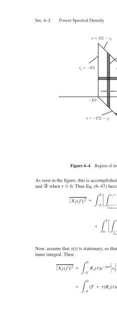
Figure 6–4 Region of integration for Eqs. (6–47) and (6–48).<br />
As seen in the figure, this is accomplished by covering the total area by using 2 when t 6 0<br />
and 3 when t 0. Thus Eq. (6–47) becomes<br />
0 t 1 = T/2<br />
ƒ X T (f) ƒ 2 = c<br />
L L<br />
2<br />
3<br />
(6–48)<br />
Now, assume that x(t) is stationary, so that R x (t 1 , t 1 t) = R x (t), and factor R x (t) outside the<br />
inner integral. Then<br />
0<br />
ƒ X T (f) ƒ 2 = R x (t)e -jvt ct 1 -<br />
L<br />
-T<br />
0<br />
T<br />
= (T + t)R x (t)e -jvt dt + (T - t)R x (t)e -jvt dt<br />
L L<br />
-T<br />
-T<br />
T t 1 = T/2-t<br />
+ c R x (t 1 , t 1 + t)e -jvt dt 1 d dt<br />
L L<br />
0<br />
t 1 = -T/2- t<br />
⎧ ⎪⎪⎪⎪⎪⎪⎪⎪⎪⎨⎪⎪⎪⎪⎪⎪⎪⎪⎪⎩<br />
t 1 = -T/2<br />
⎧ ⎪⎪⎪⎪⎪⎪⎪⎪⎪⎨⎪⎪⎪⎪⎪⎪⎪⎪⎪⎩<br />
T/2<br />
T/2-t<br />
R x (t 1, t 1 + t)e -jvt dt 1 d dt<br />
T<br />
d dt + R(t)e -jvt ct 1`<br />
L<br />
0<br />
0<br />
T/2-t d dt<br />
-T/2


