- Page 2:
Abbreviations AC ADC ADM AM ANSI AP
- Page 6:
DIGITAL AND ANALOG COMMUNICATION SY
- Page 10:
CONTENTS PREFACE LIST OF SYMBOLS xi
- Page 14:
Contents v 2-8 Discrete Fourier Tra
- Page 18:
Contents vii 4-16 Transmitters and
- Page 22:
Contents ix 6-10 Appendix: Proof of
- Page 26:
Contents xi 8-11 Wireless Data Netw
- Page 30:
PREFACE Continuing the tradition of
- Page 34:
Preface xv THE PRACTICAL APPLICATIO
- Page 38:
LIST OF SYMBOLS There are not enoug
- Page 42:
List of Symbols xix l an integer n
- Page 46:
List of Symbols xxi DEFINED FUNCTIO
- Page 50:
C h a p t e r INTRODUCTION CHAPTER
- Page 54:
Sec. 1-1 Historical Perspective 3 s
- Page 58:
Sec. 1-2 Digital and Analog Sources
- Page 62:
Sec. 1-4 Organization of the Book 7
- Page 66:
Sec. 1-6 Block Diagram of a Communi
- Page 70: Sec. 1-7 Frequency Allocations 11 T
- Page 74: Sec. 1-8 Propagation of Electromagn
- Page 78: Sec. 1-8 Propagation of Electromagn
- Page 82: Sec. 1-9 Information Measure 17 In
- Page 86: Sec. 1-10 Channel Capacity and Idea
- Page 90: Sec. 1-11 Coding 21 Transmitter Noi
- Page 94: Sec. 1-11 Coding 23 Convolutional C
- Page 98: Sec. 1-11 Coding 25 0 1 0 (00) Path
- Page 102: Sec. 1-11 Coding 27 10 -1 P e = Pro
- Page 106: Sec. 1-11 Coding 29 TABLE 1-4 CODIN
- Page 110: Problems 31 Solution: Using Eq. (1-
- Page 114: Problems 33 1-17 Using the definiti
- Page 118: Sec. 2-1 Properties of Signals and
- Page 124: 38 Signals and Spectra Chap. 2 For
- Page 128: 40 Signals and Spectra Chap. 2 V dc
- Page 132: 42 Signals and Spectra Chap. 2 aver
- Page 136: 44 Signals and Spectra Chap. 2 wher
- Page 140: 46 Signals and Spectra Chap. 2 Thes
- Page 144: 48 Signals and Spectra Chap. 2 The
- Page 148: 50 Signals and Spectra Chap. 2 Inte
- Page 152: 52 Signals and Spectra Chap. 2 TABL
- Page 156: 54 Signals and Spectra Chap. 2 Exam
- Page 160: 56 Signals and Spectra Chap. 2 DEFI
- Page 164: ( ( 58 Signals and Spectra Chap. 2
- Page 168: 60 Signals and Spectra Chap. 2 Usin
- Page 172:
62 Signals and Spectra Chap. 2 t w
- Page 176:
64 Signals and Spectra Chap. 2 TABL
- Page 180:
66 Signals and Spectra Chap. 2 wher
- Page 184:
68 Signals and Spectra Chap. 2 Orth
- Page 188:
70 Signals and Spectra Chap. 2 obta
- Page 192:
72 Signals and Spectra Chap. 2 2. I
- Page 196:
74 Signals and Spectra Chap. 2 Pola
- Page 200:
76 Signals and Spectra Chap. 2 PROO
- Page 204:
78 Signals and Spectra Chap. 2 w(t)
- Page 208:
80 Signals and Spectra Chap. 2 PROO
- Page 212:
82 Signals and Spectra Chap. 2 Inpu
- Page 216:
84 Signals and Spectra Chap. 2 is t
- Page 220:
86 Signals and Spectra Chap. 2 From
- Page 224:
88 Signals and Spectra Chap. 2 0 dB
- Page 228:
90 Signals and Spectra Chap. 2 Band
- Page 232:
92 Signals and Spectra Chap. 2 f s
- Page 236:
94 Signals and Spectra Chap. 2 w s
- Page 240:
96 Signals and Spectra Chap. 2 W(f)
- Page 244:
98 Signals and Spectra Chap. 2 MATL
- Page 248:
100 Signals and Spectra Chap. 2 aga
- Page 252:
102 Signals and Spectra Chap. 2 TAB
- Page 256:
104 Signals and Spectra Chap. 2 We
- Page 260:
106 Signals and Spectra Chap. 2 5 T
- Page 264:
108 Signals and Spectra Chap. 2 A =
- Page 268:
110 Signals and Spectra Chap. 2 the
- Page 272:
112 Signals and Spectra Chap. 2 rep
- Page 276:
114 Signals and Spectra Chap. 2 Sol
- Page 280:
116 Signals and Spectra Chap. 2 Sol
- Page 284:
118 Signals and Spectra Chap. 2 v(t
- Page 288:
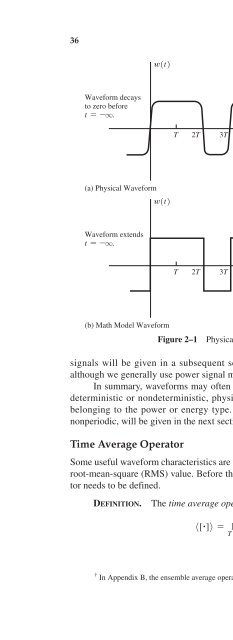
120 w(t) Signals and Spectra Chap.
- Page 292:
122 Signals and Spectra Chap. 2 2-3
- Page 296:
124 Signals and Spectra Chap. 2 ★
- Page 300:
126 Signals and Spectra Chap. 2 2-6
- Page 304:
128 Signals and Spectra Chap. 2 0.0
- Page 308:
ƒ ƒ ƒ ƒ 130 Signals and Spectra
- Page 312:
C h a p t e r BASEBAND PULSE AND DI
- Page 316:
134 Baseband Pulse and Digital Sign
- Page 320:
136 Baseband Pulse and Digital Sign
- Page 324:
138 Baseband Pulse and Digital Sign
- Page 328:
140 Baseband Pulse and Digital Sign
- Page 332:
142 Baseband Pulse and Digital Sign
- Page 336:
144 Baseband Pulse and Digital Sign
- Page 340:
146 Baseband Pulse and Digital Sign
- Page 344:
148 Baseband Pulse and Digital Sign
- Page 348:
150 Baseband Pulse and Digital Sign
- Page 352:
152 Baseband Pulse and Digital Sign
- Page 356:
154 Baseband Pulse and Digital Sign
- Page 360:
156 Baseband Pulse and Digital Sign
- Page 364:
158 Baseband Pulse and Digital Sign
- Page 368:
160 Baseband Pulse and Digital Sign
- Page 372:
162 Baseband Pulse and Digital Sign
- Page 376:
164 Baseband Pulse and Digital Sign
- Page 380:
166 Baseband Pulse and Digital Sign
- Page 384:
168 Baseband Pulse and Digital Sign
- Page 388:
170 Baseband Pulse and Digital Sign
- Page 392:
172 Baseband Pulse and Digital Sign
- Page 396:
174 Baseband Pulse and Digital Sign
- Page 400:
176 Baseband Pulse and Digital Sign
- Page 404:
178 Baseband Pulse and Digital Sign
- Page 408:
180 Baseband Pulse and Digital Sign
- Page 412:
182 Baseband Pulse and Digital Sign
- Page 416:
184 Baseband Pulse and Digital Sign
- Page 420:
186 Baseband Pulse and Digital Sign
- Page 424:
188 Baseband Pulse and Digital Sign
- Page 428:
190 Baseband Pulse and Digital Sign
- Page 432:
( 192 Baseband Pulse and Digital Si
- Page 436:
194 Baseband Pulse and Digital Sign
- Page 440:
196 DPCM transmitter Analog input s
- Page 444:
198 Baseband Pulse and Digital Sign
- Page 448:
200 Baseband Pulse and Digital Sign
- Page 452:
202 Baseband Pulse and Digital Sign
- Page 456:
204 Baseband Pulse and Digital Sign
- Page 460:
206 Baseband Pulse and Digital Sign
- Page 464:
208 Baseband Pulse and Digital Sign
- Page 468:
210 Baseband Pulse and Digital Sign
- Page 472:
212 Baseband Pulse and Digital Sign
- Page 476:
214 24 DS-0 inputs, 64 kb/s each (1
- Page 480:
216 TABLE 3-9 SPECIFICATIONS FOR T-
- Page 484:
218 Baseband Pulse and Digital Sign
- Page 488:
220 Baseband Pulse and Digital Sign
- Page 492:
222 Baseband Pulse and Digital Sign
- Page 496:
224 Baseband Pulse and Digital Sign
- Page 500:
226 Baseband Pulse and Digital Sign
- Page 504:
228 Baseband Pulse and Digital Sign
- Page 508:
230 Baseband Pulse and Digital Sign
- Page 512:
232 Baseband Pulse and Digital Sign
- Page 516:
234 Baseband Pulse and Digital Sign
- Page 520:
236 Baseband Pulse and Digital Sign
- Page 524:
238 Bandpass Signaling Principles a
- Page 528:
240 Bandpass Signaling Principles a
- Page 532:
242 TABLE 4-1 COMPLEX ENVELOPE FUNC
- Page 536:
244 Bandpass Signaling Principles a
- Page 540:
246 Bandpass Signaling Principles a
- Page 544:
248 Bandpass Signaling Principles a
- Page 548:
250 Bandpass Signaling Principles a
- Page 552:
252 Bandpass Signaling Principles a
- Page 556:
254 Bandpass Signaling Principles a
- Page 560:
256 Bandpass Signaling Principles a
- Page 564:
258 Bandpass Signaling Principles a
- Page 568:
260 Bandpass Signaling Principles a
- Page 572:
262 Bandpass Signaling Principles a
- Page 576:
264 Bandpass Signaling Principles a
- Page 580:
266 Bandpass Signaling Principles a
- Page 584:
268 Bandpass Signaling Principles a
- Page 588:
270 Bandpass Signaling Principles a
- Page 592:
272 Bandpass Signaling Principles a
- Page 596:
274 Bandpass Signaling Principles a
- Page 600:
276 Bandpass Signaling Principles a
- Page 604:
278 Bandpass Signaling Principles a
- Page 608:
280 Bandpass Signaling Principles a
- Page 612:
282 Bandpass Signaling Principles a
- Page 616:
284 Bandpass Signaling Principles a
- Page 620:
286 Bandpass Signaling Principles a
- Page 624:
288 Bandpass Signaling Principles a
- Page 628:
290 Bandpass Signaling Principles a
- Page 632:
292 Bandpass Signaling Principles a
- Page 636:
294 Bandpass Signaling Principles a
- Page 640:
296 Bandpass Signaling Principles a
- Page 644:
298 Bandpass Signaling Principles a
- Page 648:
300 Bandpass Signaling Principles a
- Page 652:
302 Bandpass Signaling Principles a
- Page 656:
304 Bandpass Signaling Principles a
- Page 660:
306 Bandpass Signaling Principles a
- Page 664:
308 Bandpass Signaling Principles a
- Page 668:
310 Bandpass Signaling Principles a
- Page 672:
312 Bandpass Signaling Principles a
- Page 676:
314 AM, FM, and Digital Modulated S
- Page 680:
316 AM, FM, and Digital Modulated S
- Page 684:
318 AM, FM, and Digital Modulated S
- Page 688:
320 TABLE 5-1 AM BROADCAST STATION
- Page 692:
322 AM, FM, and Digital Modulated S
- Page 696:
324 AM, FM, and Digital Modulated S
- Page 700:
326 AM, FM, and Digital Modulated S
- Page 704:
328 AM, FM, and Digital Modulated S
- Page 708:
330 AM, FM, and Digital Modulated S
- Page 712:
332 AM, FM, and Digital Modulated S
- Page 716:
334 AM, FM, and Digital Modulated S
- Page 720:
336 AM, FM, and Digital Modulated S
- Page 724:
338 TABLE 5-2 FOUR-PLACE VALUES OF
- Page 728:
340 AM, FM, and Digital Modulated S
- Page 732:
342 AM, FM, and Digital Modulated S
- Page 736:
344 AM, FM, and Digital Modulated S
- Page 740:
346 AM, FM, and Digital Modulated S
- Page 744:
348 AM, FM, and Digital Modulated S
- Page 748:
350 AM, FM, and Digital Modulated S
- Page 752:
352 AM, FM, and Digital Modulated S
- Page 756:
354 AM, FM, and Digital Modulated S
- Page 760:
356 AM, FM, and Digital Modulated S
- Page 764:
358 AM, FM, and Digital Modulated S
- Page 768:
360 AM, FM, and Digital Modulated S
- Page 772:
362 AM, FM, and Digital Modulated S
- Page 776:
364 AM, FM, and Digital Modulated S
- Page 780:
366 AM, FM, and Digital Modulated S
- Page 784:
368 AM, FM, and Digital Modulated S
- Page 788:
370 AM, FM, and Digital Modulated S
- Page 792:
TABLE 5-6 V.32 MODEM STANDARD Item
- Page 796:
374 AM, FM, and Digital Modulated S
- Page 800:
376 AM, FM, and Digital Modulated S
- Page 804:
378 AM, FM, and Digital Modulated S
- Page 808:
380 AM, FM, and Digital Modulated S
- Page 812:
382 AM, FM, and Digital Modulated S
- Page 816:
384 AM, FM, and Digital Modulated S
- Page 820:
386 Baseband signal processing RF c
- Page 824:
388 AM, FM, and Digital Modulated S
- Page 828:
390 AM, FM, and Digital Modulated S
- Page 832:
392 AM, FM, and Digital Modulated S
- Page 836:
394 AM, FM, and Digital Modulated S
- Page 840:
396 AM, FM, and Digital Modulated S
- Page 844:
398 AM, FM, and Digital Modulated S
- Page 848:
400 AM, FM, and Digital Modulated S
- Page 852:
402 AM, FM, and Digital Modulated S
- Page 856:
404 AM, FM, and Digital Modulated S
- Page 860:
406 AM, FM, and Digital Modulated S
- Page 864:
408 AM, FM, and Digital Modulated S
- Page 868:
410 AM, FM, and Digital Modulated S
- Page 872:
412 AM, FM, and Digital Modulated S
- Page 876:
C h a p t e r RANDOM PROCESSES AND
- Page 880:
416 Random Processes and Spectral A
- Page 884:
418 Random Processes and Spectral A
- Page 888:
420 Random Processes and Spectral A
- Page 892:
422 Random Processes and Spectral A
- Page 896:
424 Random Processes and Spectral A
- Page 900:
426 Random Processes and Spectral A
- Page 904:
428 Random Processes and Spectral A
- Page 908:
430 Random Processes and Spectral A
- Page 912:
432 Random Processes and Spectral A
- Page 916:
434 Random Processes and Spectral A
- Page 920:
436 Random Processes and Spectral A
- Page 924:
438 Random Processes and Spectral A
- Page 928:
440 Random Processes and Spectral A
- Page 932:
442 Random Processes and Spectral A
- Page 936:
444 Random Processes and Spectral A
- Page 940:
446 Random Processes and Spectral A
- Page 944:
448 Random Processes and Spectral A
- Page 948:
450 Random Processes and Spectral A
- Page 952:
452 will be WSS if and only if and
- Page 956:
454 Random Processes and Spectral A
- Page 960:
456 Random Processes and Spectral A
- Page 964:
458 Random Processes and Spectral A
- Page 968:
460 Random Processes and Spectral A
- Page 972:
462 Random Processes and Spectral A
- Page 976:
464 Random Processes and Spectral A
- Page 980:
466 Random Processes and Spectral A
- Page 984:
468 Random Processes and Spectral A
- Page 988:
470 Random Processes and Spectral A
- Page 992:
472 Random Processes and Spectral A
- Page 996:
474 Random Processes and Spectral A
- Page 1000:
476 Random Processes and Spectral A
- Page 1004:
478 Random Processes and Spectral A
- Page 1008:
480 Random Processes and Spectral A
- Page 1012:
482 Random Processes and Spectral A
- Page 1016:
484 Random Processes and Spectral A
- Page 1020:
486 Random Processes and Spectral A
- Page 1024:
488 Random Processes and Spectral A
- Page 1028:
490 Random Processes and Spectral A
- Page 1032:
C h a p t e r PERFORMANCE OF COMMUN
- Page 1036:
494 Performance of Communication Sy
- Page 1040:
496 Performance of Communication Sy
- Page 1044:
498 Performance of Communication Sy
- Page 1048:
500 Performance of Communication Sy
- Page 1052:
502 Performance of Communication Sy
- Page 1056:
504 Performance of Communication Sy
- Page 1060:
506 Performance of Communication Sy
- Page 1064:
508 Upper channel Receiver r(t)=s(t
- Page 1068:
510 Performance of Communication Sy
- Page 1072:
512 Performance of Communication Sy
- Page 1076:
514 Performance of Communication Sy
- Page 1080:
516 Performance of Communication Sy
- Page 1084:
518 DPSK signal plus noise in Bandp
- Page 1088:
520 QPSK signal plus noise (data ra
- Page 1092:
TABLE 7-1 COMPARISON OF DIGITALSIGN
- Page 1096:
524 Performance of Communication Sy
- Page 1100:
526 Performance of Communication Sy
- Page 1104:
528 Performance of Communication Sy
- Page 1108:
530 Performance of Communication Sy
- Page 1112:
532 Performance of Communication Sy
- Page 1116:
534 Performance of Communication Sy
- Page 1120:
536 Performance of Communication Sy
- Page 1124:
538 Performance of Communication Sy
- Page 1128:
540 Performance of Communication Sy
- Page 1132:
542 Performance of Communication Sy
- Page 1136:
544 Performance of Communication Sy
- Page 1140:
546 Performance of Communication Sy
- Page 1144:
548 Performance of Communication Sy
- Page 1148:
550 Performance of Communication Sy
- Page 1152:
552 Performance of Communication Sy
- Page 1156:
554 Performance of Communication Sy
- Page 1160:
556 Performance of Communication Sy
- Page 1164:
558 Performance of Communication Sy
- Page 1168:
560 Performance of Communication Sy
- Page 1172:
562 Performance of Communication Sy
- Page 1176:
564 Performance of Communication Sy
- Page 1180:
- f c f c f 566 Performance of Comm
- Page 1184:
568 Performance of Communication Sy
- Page 1188:
570 Wire and Wireless Communication
- Page 1192:
572 Wire and Wireless Communication
- Page 1196:
574 Wire and Wireless Communication
- Page 1200:
576 Tip (green wire) POTS line card
- Page 1204:
578 Wire and Wireless Communication
- Page 1208:
580 Wire and Wireless Communication
- Page 1212:
582 Wire and Wireless Communication
- Page 1216:
TABLE 8-2 CAPACITY OF PUBLIC-SWITCH
- Page 1220:
586 Wire and Wireless Communication
- Page 1224:
588 Wire and Wireless Communication
- Page 1228:
590 Wire and Wireless Communication
- Page 1232:
592 Wire and Wireless Communication
- Page 1236:
594 Wire and Wireless Communication
- Page 1240:
596 Wire and Wireless Communication
- Page 1244:
598 Wire and Wireless Communication
- Page 1248:
600 Wire and Wireless Communication
- Page 1252:
602 Wire and Wireless Communication
- Page 1256:
604 Wire and Wireless Communication
- Page 1260:
606 Wire and Wireless Communication
- Page 1264:
608 Wire and Wireless Communication
- Page 1268:
( 610 Wire and Wireless Communicati
- Page 1272:
612 Wire and Wireless Communication
- Page 1276:
614 Wire and Wireless Communication
- Page 1280:
616 Wire and Wireless Communication
- Page 1284:
618 Wire and Wireless Communication
- Page 1288:
620 Wire and Wireless Communication
- Page 1292:
622 Wire and Wireless Communication
- Page 1296:
624 Wire and Wireless Communication
- Page 1300:
626 Wire and Wireless Communication
- Page 1304:
628 Wire and Wireless Communication
- Page 1308:
630 Wire and Wireless Communication
- Page 1312:
632 Wire and Wireless Communication
- Page 1316:
634 Wire and Wireless Communication
- Page 1320:
636 Wire and Wireless Communication
- Page 1324:
638 Wire and Wireless Communication
- Page 1328:
ƒ ƒ 640 Wire and Wireless Communi
- Page 1332:
642 Wire and Wireless Communication
- Page 1336:
644 Wire and Wireless Communication
- Page 1340:
Channel Broadcast On-the-Air Channe
- Page 1344:
Channel Broadcast On-the-Air Channe
- Page 1348:
650 Wire and Wireless Communication
- Page 1352:
652 Wire and Wireless Communication
- Page 1356:
654 Wire and Wireless Communication
- Page 1360:
656 Wire and Wireless Communication
- Page 1364:
658 Wire and Wireless Communication
- Page 1368:
660 Wire and Wireless Communication
- Page 1372:
662 Wire and Wireless Communication
- Page 1376:
664 Wire and Wireless Communication
- Page 1380:
666 Wire and Wireless Communication
- Page 1384:
668 Wire and Wireless Communication
- Page 1388:
670 Mathematical Techniques, Identi
- Page 1392:
672 Mathematical Techniques, Identi
- Page 1396:
674 Mathematical Techniques, Identi
- Page 1400:
676 Mathematical Techniques, Identi
- Page 1404:
678 A-10 TABULATION OF Q (z) Mathem
- Page 1408:
A p p e n d i x PROBABILITY AND RAN
- Page 1412:
682 Probability and Random Variable
- Page 1416:
684 which is identical to Eq. (B-4)
- Page 1420:
686 Probability and Random Variable
- Page 1424:
688 Probability and Random Variable
- Page 1428:
690 Probability and Random Variable
- Page 1432:
692 Probability and Random Variable
- Page 1436:
694 Probability and Random Variable
- Page 1440:
TABLE B-1 SOME DISTRIBUTIONS AND TH
- Page 1444:
698 Probability and Random Variable
- Page 1448:
700 Probability and Random Variable
- Page 1452:
702 Probability and Random Variable
- Page 1456:
ƒ ƒ 704 Probability and Random Va
- Page 1460:
706 Probability and Random Variable
- Page 1464:
708 Probability and Random Variable
- Page 1468:
710 3. F(a 1 , a 2 ,..., a N ) Prob
- Page 1472:
712 Probability and Random Variable
- Page 1476:
714 Probability and Random Variable
- Page 1480:
716 Probability and Random Variable
- Page 1484:
718 Probability and Random Variable
- Page 1488:
720 Probability and Random Variable
- Page 1492:
722 Probability and Random Variable
- Page 1496:
724 Using MATLAB Appendix C Of cour
- Page 1500:
726 Using MATLAB Appendix C 6. The
- Page 1504:
728 References AT&T, FT-2000 OC-48
- Page 1508:
730 References COUCH, L. W., Digita
- Page 1512:
732 References HAMMING, R. W., “E
- Page 1516:
734 References LIN, D. W., C. CHEN,
- Page 1520:
736 References PRITCHARD, W. L., an
- Page 1524:
738 References UNGERBOECK, G., “C
- Page 1528:
740 Answers to Selected Problems Ch
- Page 1532:
742 Answers to Selected Problems 2
- Page 1536:
744 Answers to Selected Problems 5-
- Page 1540:
746 Answers to Selected Problems h
- Page 1544:
748 Index Amplitude shift keying (A
- Page 1548:
750 Index Coding/codes (cont.) chan
- Page 1552:
752 Index Effective isotropic radia
- Page 1556:
754 Index In-phase components, 638
- Page 1560:
756 Index Multilevel signaling, 157
- Page 1564:
758 Index Process/processing (cont.
- Page 1568:
760 Index Signal/signaling (cont.)
- Page 1572:
762 Index Two-level data, 165 Two-q
- Page 1576:
TABLE 2-2 SOME FOURIER TRANSFORM PA


![Genki - An Integrated Course in Elementary Japanese II [Second Edition] (2011), WITH PDF BOOKMARKS!](https://img.yumpu.com/58322134/1/180x260/genki-an-integrated-course-in-elementary-japanese-ii-second-edition-2011-with-pdf-bookmarks.jpg?quality=85)
![Genki - An Integrated Course in Elementary Japanese I [Second Edition] (2011), WITH PDF BOOKMARKS!](https://img.yumpu.com/58322120/1/182x260/genki-an-integrated-course-in-elementary-japanese-i-second-edition-2011-with-pdf-bookmarks.jpg?quality=85)