4569846498

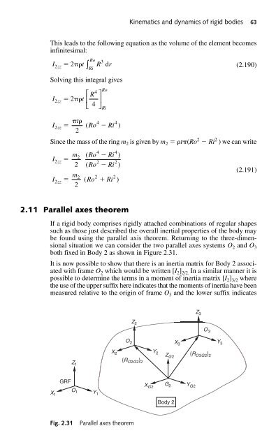
Kinematics and dynamics of rigid bodies 63
This leads to the following equation as the volume of the element becomes
infinitesimal:
Solving this integral gives
I
2zz
I
(2.190)
Since the mass of the ring m 2 is given by m 2 t(Ro 2 Ri 2 ) we can write
I
2zz
I
2zz
2zz
Ro
3
I2zz
2 t∫
R dr
Ri
4
R
2
t
⎡ ⎣ ⎢
⎤
⎥
4 ⎦
Ro
Ri
t 4 4
Ro Ri
2 ( )
4 4
m2
( Ro Ri )
2 2
2 ( Ro Ri )
m2 Ro
2 Ri
2
2 ( )
(2.191)
2.11 Parallel axes theorem
If a rigid body comprises rigidly attached combinations of regular shapes
such as those just described the overall inertial properties of the body may
be found using the parallel axis theorem. Returning to the three-dimensional
situation we can consider the two parallel axes systems O 2 and O 3
both fixed in Body 2 as shown in Figure 2.31.
It is now possible to show that there is an inertia matrix for Body 2 associated
with frame O 2 which would be written [I 2 ] 2/2. In a similar manner it is
possible to determine the terms in a moment of inertia matrix [I 2 ] 3/2 where
the use of the upper suffix here indicates that the moments of inertia have been
measured relative to the origin of frame O 3 and the lower suffix indicates
Z 3
Z 2
X 3
O 3
Y 3
O 2
X 2 Y 2
Z G2
{R O3G2 } 2
Z
{R O2G2 } 2 1
GRF
X 1
O 1
Y 1
X G2
G 2
Y G2
Body 2
Fig. 2.31
Parallel axes theorem