4569846498

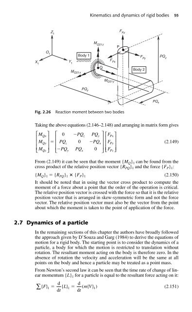
Kinematics and dynamics of rigid bodies 55
F Pz
Z 1
M Q21z
P
O 1
Body 1
F Py
X 1
Y F 1 Px
Q
M
Body 2
Q21x
M Q21y
PQ z
PQ y
PQ x
Fig. 2.26
Reaction moment between two bodies
Taking the above equations (2.146–2.148) and arranging in matrix form gives
⎡M
⎢
⎢M
⎢
⎣M
Qx
Qy
Qz
⎤ ⎡ 0
⎥ ⎢
⎥ ⎢ PQz
⎥ ⎢
⎦ ⎣
PQ
y
PQz
0
PQ
x
PQy
PQ
0
x
⎤ ⎡F
⎥ ⎢
⎥ ⎢
F
⎥
⎦ ⎣⎢
F
(2.149)
From (2.149) it can be seen that the moment {M Q } 1 can be found from the
cross product of the relative position vector {R PQ } 1 and the force {F P } 1 :
{M Q } 1 {R PQ } 1 {F P } 1 (2.150)
It should be noted that in using the vector cross product to compute the
moment of a force about a point that the order of the operation is critical.
The relative position vector is crossed with the force so that it is the relative
position vector that is arranged in skew-symmetric form and not the force
vector. The relative position vector must also be the vector from the point
about which the moment is taken to the point of application of the force.
Px
Py
Pz
⎤
⎥
⎥
⎦⎥
2.7 Dynamics of a particle
In the remaining sections of this chapter the authors have broadly followed
the approach given by D’Souza and Garg (1984) to derive the equations of
motion for a rigid body. The starting point is to consider the dynamics of a
particle, a body for which the motion is restricted to translation without
rotation. The resultant moment acting on the body is therefore zero. In the
absence of rotation the velocity and acceleration will be the same at all
points on the body and hence a particle may be treated as a point mass.
From Newton’s second law it can be seen that the time rate of change of linear
momentum {L} 1 for a particle is equal to the resultant force acting on it:
d d
∑{} F 1 {} L 1 mV {} 1
(2.151)
dt
d t
( )