4569846498
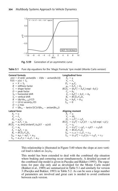
Tyre characteristics and modelling 303 y Y D arctan(BCD) y s S v x m x X S h Fig. 5.58 Coefficients used in the ‘Magic Formula’ tyre fit a particular tyre or if suitable taken as the constants given in Bakker et al. (1986): 1.30 – lateral force curve 1.65 – longitudinal braking force curve 2.40 – aligning moment curve B – is referred to as a ‘stiffness’ factor. From Figure 5.58 it can be seen that BCD is the slope at the origin, i.e. the cornering stiffness when plotting lateral force. Obtaining values for D and C leads to a value for B. E – is a ‘curvature’ factor that effects the transition in the curve and the position x m at which the peak value if present occurs. E is calculated using: E Bxm tan 2C Bx arctan Bx m ( ) ( ) m (5.52) y s – is the asymptotic value at large slip values and is found using: y s D sin(C/2) (5.53) The curvature factor E can be made dependent on the sign of the slip value plotted on the x-axis: E E 0 E sgn(x) (5.54) This will allow for the lack of symmetry between the right and left side of the diagram when comparing driving and braking forces or to introduce the effects of camber angle . This effect is illustrated in Pacejka and Bakker (1993) by the generation of an asymmetric curve using coefficients C 1.6, E O 0.5 and E 0.5. This is recreated here using the curve shape illustrated in Figure 5.59. Note that the plots have been made nondimensional by plotting y/D on the y-axis and BCx on the x-axis. The ‘Magic Formula’ utilizes a set of coefficients a 0 , a 1 , a 2 , … as shown in Tables 5.1 and 5.2. In Figure 5.60 it can be seen that at zero camber the cornering stiffness BCD y reaches a maximum value defined by the coefficient a 3 at a given value of vertical load F z that equates to the coefficient a 4 .
304 Multibody Systems Approach to Vehicle Dynamics 1.0 C 1.6 E 0.5 0.5 * sgn(x) 0.5 y/D 0.0 0.5 1.0 10 Fig. 5.59 NOT TO SCALE 8 6 4 2 0 2 4 6 8 10 BCx Generation of an asymmetric curve Table 5.1 Pure slip equations for the ‘Magic Formula’ tyre model (Monte Carlo version) General formula Longitudinal force y(x) D sin[C arctan{Bx E(Bx arctan(Bx))}] X x Y(X) y(x) S v Y x F x x X S h D x x F z B stiffness factor x b 1 F z b 2 C shape factor BCD x (b 3 F 2 z b 4 F z ) exp(b 5 F z ) D peak factor C x b 0 S h horizontal shift E x b 6 F 2 z b 7 F z b 8 S v vertical shift B x BCD x /C x D x B (dy/dx (x0) )/CD S hx b 9 F z b 10 C (2/) arcsin(y s /D) S vy 0 D y max E (Bx m tan(/2C))/(Bx m arctan(Bx m )) Lateral force Aligning moment X y X z Y y F y Y z M z D y y F z D z c 1 F 2 z c 2 F z y a 1 F z a 2 BCD z (c 3 F 2 z c 4 F z )(1 c 6 ||) exp(c 5 F z ) BCD y a 3 sin(2 arctan(F z /a 4 ))(1 a 5 ||) C z c 0 C y a 0 E z (c 7 F 2 z c 8 F z c 9 )(1 c 10 ||) E y a 6 F z a 7 B z BCD z /C z D z B y BCD y /C y D y S hz c 11 c 12 F z c 13 S hy a 8 a 9 F z a 10 S vz (c 14 F 2 z c 15 F z )c 16 F z c 17 S vy a 11 F z a 12 F z a 13 This relationship is illustrated in Figure 5.60 where the slope at zero vertical load is taken as 2a 3 /a 4 . This model has been extended to deal with the combined slip situation where braking and cornering occur simultaneously. A detailed account of the combined slip model is given in Pacejka and Bakker (1993). The equations for pure slip only and as developed for the Monte Carlo model (Bakker et al., 1989) are summarized in Table 5.1 and similarly for version 3 (Pacejka and Bakker, 1993) in Table 5.2. As can be seen a large number of parameters are involved and great care is needed to avoid confusion between each version.
- Page 276 and 277: Tyre characteristics and modelling
- Page 278 and 279: Tyre characteristics and modelling
- Page 280 and 281: Tyre characteristics and modelling
- Page 282 and 283: Tyre characteristics and modelling
- Page 284 and 285: Tyre characteristics and modelling
- Page 286 and 287: Tyre characteristics and modelling
- Page 288 and 289: Tyre characteristics and modelling
- Page 290 and 291: Tyre characteristics and modelling
- Page 292 and 293: Tyre characteristics and modelling
- Page 294 and 295: Tyre characteristics and modelling
- Page 296 and 297: Tyre characteristics and modelling
- Page 298 and 299: Tyre characteristics and modelling
- Page 300 and 301: Tyre characteristics and modelling
- Page 302 and 303: Tyre characteristics and modelling
- Page 304 and 305: Tyre characteristics and modelling
- Page 306 and 307: Tyre characteristics and modelling
- Page 308 and 309: Tyre characteristics and modelling
- Page 310 and 311: Tyre characteristics and modelling
- Page 312 and 313: Tyre characteristics and modelling
- Page 314 and 315: Tyre characteristics and modelling
- Page 316 and 317: Tyre characteristics and modelling
- Page 318 and 319: Tyre characteristics and modelling
- Page 320 and 321: Tyre characteristics and modelling
- Page 322 and 323: Tyre characteristics and modelling
- Page 324 and 325: Tyre characteristics and modelling
- Page 328 and 329: Tyre characteristics and modelling
- Page 330 and 331: Tyre characteristics and modelling
- Page 332 and 333: Tyre characteristics and modelling
- Page 334 and 335: Tyre characteristics and modelling
- Page 336 and 337: Tyre characteristics and modelling
- Page 338 and 339: Tyre characteristics and modelling
- Page 340 and 341: Tyre characteristics and modelling
- Page 342 and 343: Tyre characteristics and modelling
- Page 344 and 345: Tyre characteristics and modelling
- Page 346 and 347: Tyre characteristics and modelling
- Page 348 and 349: Tyre characteristics and modelling
- Page 350 and 351: Modelling and assembly of the full
- Page 352 and 353: Modelling and assembly of the full
- Page 354 and 355: Modelling and assembly of the full
- Page 356 and 357: Modelling and assembly of the full
- Page 358 and 359: Modelling and assembly of the full
- Page 360 and 361: Modelling and assembly of the full
- Page 362 and 363: Modelling and assembly of the full
- Page 364 and 365: Modelling and assembly of the full
- Page 366 and 367: Modelling and assembly of the full
- Page 368 and 369: Modelling and assembly of the full
- Page 370 and 371: Modelling and assembly of the full
- Page 372 and 373: Modelling and assembly of the full
- Page 374 and 375: Modelling and assembly of the full
304 Multibody Systems Approach to Vehicle Dynamics<br />
1.0<br />
C 1.6 E 0.5 0.5 * sgn(x)<br />
0.5<br />
y/D<br />
0.0<br />
0.5<br />
1.0<br />
10<br />
Fig. 5.59<br />
NOT TO SCALE<br />
8 6 4 2 0 2 4 6 8 10<br />
BCx<br />
Generation of an asymmetric curve<br />
Table 5.1<br />
Pure slip equations for the ‘Magic Formula’ tyre model (Monte Carlo version)<br />
General formula<br />
Longitudinal force<br />
y(x) D sin[C arctan{Bx E(Bx arctan(Bx))}] X x <br />
Y(X) y(x) S v<br />
Y x F x<br />
x X S h<br />
D x x F z<br />
B stiffness factor x b 1 F z b 2<br />
C shape factor BCD x (b 3 F 2 z b 4 F z ) exp(b 5 F z )<br />
D peak factor C x b 0<br />
S h horizontal shift E x b 6 F 2 z b 7 F z b 8<br />
S v vertical shift<br />
B x BCD x /C x D x<br />
B (dy/dx (x0) )/CD S hx b 9 F z b 10<br />
C (2/) arcsin(y s /D) S vy 0<br />
D y max<br />
E (Bx m tan(/2C))/(Bx m arctan(Bx m ))<br />
Lateral force<br />
Aligning moment<br />
X y X z <br />
Y y F y<br />
Y z M z<br />
D y y F z<br />
D z c 1 F 2 z c 2 F z<br />
y a 1 F z a 2 BCD z (c 3 F 2 z c 4 F z )(1 c 6 ||) exp(c 5 F z )<br />
BCD y a 3 sin(2 arctan(F z /a 4 ))(1 a 5 ||) C z c 0<br />
C y a 0<br />
E z (c 7 F 2 z c 8 F z c 9 )(1 c 10 ||)<br />
E y a 6 F z a 7<br />
B z BCD z /C z D z<br />
B y BCD y /C y D y S hz c 11 c 12 F z c 13<br />
S hy a 8 a 9 F z a 10 S vz (c 14 F 2 z c 15 F z )c 16 F z c 17<br />
S vy a 11 F z a 12 F z a 13<br />
This relationship is illustrated in Figure 5.60 where the slope at zero vertical<br />
load is taken as 2a 3 /a 4 .<br />
This model has been extended to deal with the combined slip situation<br />
where braking and cornering occur simultaneously. A detailed account of<br />
the combined slip model is given in Pacejka and Bakker (1993). The equations<br />
for pure slip only and as developed for the Monte Carlo model<br />
(Bakker et al., 1989) are summarized in Table 5.1 and similarly for version<br />
3 (Pacejka and Bakker, 1993) in Table 5.2. As can be seen a large number<br />
of parameters are involved and great care is needed to avoid confusion<br />
between each version.


