4569846498
Modelling and analysis of suspension systems 225 Equation 4 3 6x 9 6y 436 6z 0 (4.250) The four equations can now be set up in matrix form ready for solution: ⎡ 3 0 436 9 ⎤ ⎡ A s ⎤ ⎡ 669.564 ⎤ ⎢ 9 436 0 3 ⎥ ⎢ ⎥ ⎢ 28 592.484 ⎥ ⎢ ⎥ ⎢ 6x ⎥ ⎢ ⎥ (4.251) ⎢436 9 3 0 ⎥ ⎢6y ⎥ ⎢ 3838.594⎥ ⎢ ⎥ ⎢ ⎥ ⎢ ⎥ ⎣ 0 3 9 436⎦ ⎣6z ⎦ ⎣ 0 ⎦ Solving equation (4.251) yields the following answers for the four unknowns: A s 7.457 s 2 6x 65.730 rad/s 2 6y 1.147 rad/s 2 6z 0.483 rad/s 2 This gives us the last two angular acceleration vectors for the upper and lower damper bodies: T 6 1 T 7 1 { } [ 65.730 1.147 0.483 ] rad/s { } [ 65.730 1.147 0.483 ] rad/s From equation (4.240) we now have {A C6C7 } 1 2{ 6 } 1 {V C6C7 } 1 A s {R CI } 1 (4.252) ⎡879.162⎤ ⎡ 3 ⎤ ⎡ 856.791 ⎤ { A C C } 1 ⎢ 3626.702 ⎥ 7.457 ⎢ 9 ⎥ ⎢ 3559.589 ⎥ mm/s ⎢ ⎥ ⎢ ⎥ ⎢ ⎥ ⎣⎢ 80.457 ⎦⎥ ⎣⎢ 436⎦⎥ ⎣⎢ 3331.709⎦⎥ 6 7 2 (4.253) A comparison of the angular accelerations found from the preceding calculations and those found using an equivalent MSC.ADAMS model is shown in Table 4.12. 2 2 Table 4.12 Comparison of angular acceleration vectors computed by theory and MSC.ADAMS Body Angular acceleration vectors Theory MSC.ADAMS x (rad/s 2 ) y (rad/s 2 ) z (rad/s 2 ) x (rad/s 2 ) y (rad/s 2 ) z (rad/s 2 ) 2 11.790 0.0 0.0 11.791 0.0 0.0 3 18.819 0.0 1.145 18.823 0.0 1.146 4 29.386 3.737 20.847 29.395 3.737 20.840 5 23.361 0.065 1.843 23.384 0.157 2.053 6 65.730 1.147 0.483 57.204 2.663 0.449 7 65.730 1.147 0.483 57.204 2.663 0.449
226 Multibody Systems Approach to Vehicle Dynamics Table 4.13 Comparison of translational acceleration vectors computed by theory and MSC.ADAMS Point Translational acceleration vectors Theory MSC.ADAMS A x (mm/s 2 ) A y (mm/s 2 ) A z (mm/s 2 ) A x (mm/s 2 ) A y (mm/s 2 ) A z (mm/s 2 ) C 210.614 28 476.707 3455.690 210.385 28 478.60 3456.320 D 177.625 47 432.261 2920.973 177.846 47 433.70 2921.760 G 0.0 41 481.177 1888.432 0.0 41 480.60 1888.430 H 422.619 45 953.343 3744.647 420.215 45 933.00 3722.660 P 558.211 36 163.671 0.0 557.780 36 161.60 0.0 C 6 C 7 856.791 3559.589 3331.709 957.170 3 544.09 2566.940 A comparison of the translational accelerations found at points within the suspension system from the preceding calculations and those found using an equivalent MSC.ADAMS model is shown in Table 4.13. 4.10.4 Static analysis As discussed in this chapter a starting point for suspension component loading studies is to use equivalent static forces to represent the loads acting through the road wheel, associated with real world driving conditions. In this example the vector analysis method is used to carry out a static analysis where a vertical load of 10 000 N is applied at the tyre contact patch, this being representative in magnitude of the loads used for a 3G bump case on a typical vehicle of this size. In this analysis we are ignoring gravity and the self-weight of the suspension components as this contribution tends to be minor compared with overall vehicle loads reacted at the tyre contact patch and diffused into the suspension system. For completeness the effects of self-weight will be included in a follow-on demonstration of a dynamic analysis. Before attempting any vector analysis to determine the distribution of forces it is necessary to prepare a free-body diagram and label the bodies and forces in an appropriate manner as shown in Figure 4.73. For the action–reaction forces shown acting between the bodies in Figure 4.73 Newton’s third law would apply. The interaction, for example, at point D between Body 3 and Body 4 requires {F D43 } 1 and {F D34 } 1 to be equal and opposite equal. Thus instead of including the six unknowns F D43x , F D43y , F D43z , F D34x , F D34y and F D34z we can reduce this to three unknowns F D43x , F D43y , F D43z . In a similar manner looking at the connections at points G and H we can see for all connections to Body 4 that the following applies: {F D43 } 1 {F D34 } 1 (4.254) {F G42 } 1 {F G24 } 1 (4.255) {F H45 } 1 {F H54 } 1 (4.256)
- Page 198 and 199: Modelling and analysis of suspensio
- Page 200 and 201: Modelling and analysis of suspensio
- Page 202 and 203: Modelling and analysis of suspensio
- Page 204 and 205: Modelling and analysis of suspensio
- Page 206 and 207: Modelling and analysis of suspensio
- Page 208 and 209: Modelling and analysis of suspensio
- Page 210 and 211: Modelling and analysis of suspensio
- Page 212 and 213: Modelling and analysis of suspensio
- Page 214 and 215: Modelling and analysis of suspensio
- Page 216 and 217: Modelling and analysis of suspensio
- Page 218 and 219: Modelling and analysis of suspensio
- Page 220 and 221: Modelling and analysis of suspensio
- Page 222 and 223: Modelling and analysis of suspensio
- Page 224 and 225: Modelling and analysis of suspensio
- Page 226 and 227: Modelling and analysis of suspensio
- Page 228 and 229: Modelling and analysis of suspensio
- Page 230 and 231: Modelling and analysis of suspensio
- Page 232 and 233: Modelling and analysis of suspensio
- Page 234 and 235: Modelling and analysis of suspensio
- Page 236 and 237: Modelling and analysis of suspensio
- Page 238 and 239: Modelling and analysis of suspensio
- Page 240 and 241: Modelling and analysis of suspensio
- Page 242 and 243: Modelling and analysis of suspensio
- Page 244 and 245: Modelling and analysis of suspensio
- Page 246 and 247: Modelling and analysis of suspensio
- Page 250 and 251: Modelling and analysis of suspensio
- Page 252 and 253: Modelling and analysis of suspensio
- Page 254 and 255: Modelling and analysis of suspensio
- Page 256 and 257: Modelling and analysis of suspensio
- Page 258 and 259: Modelling and analysis of suspensio
- Page 260 and 261: Modelling and analysis of suspensio
- Page 262 and 263: Modelling and analysis of suspensio
- Page 264 and 265: Modelling and analysis of suspensio
- Page 266 and 267: Modelling and analysis of suspensio
- Page 268 and 269: Modelling and analysis of suspensio
- Page 270 and 271: Modelling and analysis of suspensio
- Page 272 and 273: Tyre characteristics and modelling
- Page 274 and 275: Tyre characteristics and modelling
- Page 276 and 277: Tyre characteristics and modelling
- Page 278 and 279: Tyre characteristics and modelling
- Page 280 and 281: Tyre characteristics and modelling
- Page 282 and 283: Tyre characteristics and modelling
- Page 284 and 285: Tyre characteristics and modelling
- Page 286 and 287: Tyre characteristics and modelling
- Page 288 and 289: Tyre characteristics and modelling
- Page 290 and 291: Tyre characteristics and modelling
- Page 292 and 293: Tyre characteristics and modelling
- Page 294 and 295: Tyre characteristics and modelling
- Page 296 and 297: Tyre characteristics and modelling
226 Multibody Systems Approach to Vehicle Dynamics<br />
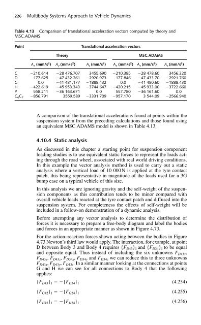
Table 4.13 Comparison of translational acceleration vectors computed by theory and<br />
MSC.ADAMS<br />
Point<br />
Translational acceleration vectors<br />
Theory<br />
MSC.ADAMS<br />
A x (mm/s 2 ) A y (mm/s 2 ) A z (mm/s 2 ) A x (mm/s 2 ) A y (mm/s 2 ) A z (mm/s 2 )<br />
C 210.614 28 476.707 3455.690 210.385 28 478.60 3456.320<br />
D 177.625 47 432.261 2920.973 177.846 47 433.70 2921.760<br />
G 0.0 41 481.177 1888.432 0.0 41 480.60 1888.430<br />
H 422.619 45 953.343 3744.647 420.215 45 933.00 3722.660<br />
P 558.211 36 163.671 0.0 557.780 36 161.60 0.0<br />
C 6 C 7 856.791 3559.589 3331.709 957.170 3 544.09 2566.940<br />
A comparison of the translational accelerations found at points within the<br />
suspension system from the preceding calculations and those found using<br />
an equivalent MSC.ADAMS model is shown in Table 4.13.<br />
4.10.4 Static analysis<br />
As discussed in this chapter a starting point for suspension component<br />
loading studies is to use equivalent static forces to represent the loads acting<br />
through the road wheel, associated with real world driving conditions.<br />
In this example the vector analysis method is used to carry out a static<br />
analysis where a vertical load of 10 000 N is applied at the tyre contact<br />
patch, this being representative in magnitude of the loads used for a 3G<br />
bump case on a typical vehicle of this size.<br />
In this analysis we are ignoring gravity and the self-weight of the suspension<br />
components as this contribution tends to be minor compared with<br />
overall vehicle loads reacted at the tyre contact patch and diffused into the<br />
suspension system. For completeness the effects of self-weight will be<br />
included in a follow-on demonstration of a dynamic analysis.<br />
Before attempting any vector analysis to determine the distribution of<br />
forces it is necessary to prepare a free-body diagram and label the bodies<br />
and forces in an appropriate manner as shown in Figure 4.73.<br />
For the action–reaction forces shown acting between the bodies in Figure<br />
4.73 Newton’s third law would apply. The interaction, for example, at point<br />
D between Body 3 and Body 4 requires {F D43 } 1 and {F D34 } 1 to be equal<br />
and opposite equal. Thus instead of including the six unknowns F D43x ,<br />
F D43y , F D43z , F D34x , F D34y and F D34z we can reduce this to three unknowns<br />
F D43x , F D43y , F D43z . In a similar manner looking at the connections at points<br />
G and H we can see for all connections to Body 4 that the following<br />
applies:<br />
{F D43 } 1 {F D34 } 1 (4.254)<br />
{F G42 } 1 {F G24 } 1 (4.255)<br />
{F H45 } 1 {F H54 } 1 (4.256)


