4569846498

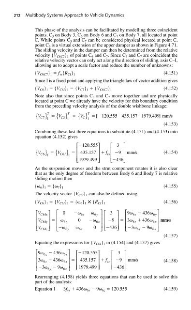
212 Multibody Systems Approach to Vehicle Dynamics
This phase of the analysis can be facilitated by modelling three coincident
points, C 3 on Body 3, C 6 on Body 6 and C 7 on Body 7, all located at point
C. While points C 3 and C 7 can be considered physical located at point C,
point C 6 is a virtual extension of the upper damper as shown in Figure 4.71.
The sliding velocity in the damper can then be determined from the relative
velocity {V C6C7 } 1 of points C 6 and C 7 . Since C 6 and C 7 are coincident the
relative velocity vector can only act along the direction of sliding, axis C–I,
allowing us to adopt a scale factor and reduce the number of unknowns:
{V C6C7 } 1 f vs {R CI } 1 (4.151)
Since I is a fixed point and applying the triangle law of vector addition gives
{V C6 } 1 {V C6I } 1 {V C7 } 1 {V C6C7 } 1 (4.152)
Note also that since points C 3 and C 7 move together and are physically
located at point C we already have the velocity for this boundary condition
from the preceding velocity analysis of the double wishbone linkage:
{ } { } { }
(4.153)
Combining these last three equations to substitute (4.151) and (4.153) into
equation (4.152) gives
⎡120.555⎤
⎡ 3 ⎤
{ VC6 } 1
{ VC6
I}
⎢
435.157
⎥
f
⎢
vs 9
⎥
mm/s
(4.154)
1 ⎢ ⎥ ⎢ ⎥
⎣⎢
1979.499 ⎦⎥
⎣⎢
436⎦⎥
As the suspension moves and the strut component rotates it is also clear
that as the only degree of freedom between Body 6 and Body 7 is relative
sliding motion then
{ 6 } 1 { 7 } 1 (4.155)
The velocity vector {V C6I } 1 can also be defined using
{V C6 } 1 {V C6I } 1 { 6 } 1 {R CI } 1 (4.156)
⎡V
⎢
⎢
V
⎣⎢
V
T
T
T
C7 1 C3 1 C 1
V V = V [ 120.555 435.157 1979.499 ] mm/s
C6Ix
C6Iy
C6Iz
⎤ ⎡ 0
⎥ ⎢
⎥
⎢
⎦⎥
⎢
⎣
Equating the expressions for {V C6I } 1 in (4.154) and (4.157) gives
⎡9 z 436
⎢
⎢3 z 436
⎢
⎣
3 y 9
6 6y
6 6x
6 6x
0
6z
6y
6z
6x
6y
6x
0
⎤ ⎡120.555⎤
⎥
⎢
⎥ 435.157
⎥
⎢ ⎥
⎥
⎦ ⎣⎢
1979.499 ⎦⎥
⎤ ⎡ 3 ⎤ ⎡9 436
⎥ ⎢
⎥ 9
⎥ ⎢
3 436
⎢ ⎥ ⎢
⎥
⎦ ⎣⎢
436⎦⎥
⎢
⎣
3 9
f vs
⎡ 3 ⎤
⎢
9
⎥
mm/s
⎢ ⎥
⎣⎢
436⎦⎥
6z
6y
6z
6x
6y
6x
(4.157)
(4.158)
Rearranging (4.158) yields three equations that can be used to solve this
part of the analysis:
Equation 1 3f vs 436 6y 9 6z 120.555 (4.159)
⎤
⎥
⎥
⎥
⎦
mm/s