4569846498
Modelling and analysis of suspension systems 183 Once generated the suspension model may be used in two ways. One of these is to apply the load and carry out a static analysis. This may result in the suspension system moving through relatively large displacement to obtain a static equilibrium position for the given load. The static reactions in joints, bushes and spring seats can then be extracted. It is also possible to make the load a function of time and then to apply a quasi-static analysis. This has the advantage that the graphical post-processor can be used to animate the simulation to demonstrate how the suspension moves under the given load. An example of this for the 3G bump case would be to apply the 1G load for an initial static analysis at time equal to zero and then to apply the remaining 2G of the load over, say, 1 second of simulation time. The use of equivalent static loads to represent real dynamic effects has been used by the automotive industry for some time. The derivation of design loads similar to those shown in Table 4.8 can be traced back to a publication in the early 1950s (Garrett, 1953) in the Automobile Engineer. The disadvantage of the static analysis is that any velocity dependent forces will not be transmitted through the damper without the inclusion of some static equivalent. The extension of this is to carry out a dynamic simulation if possible. The model used may be a quarter suspension model or even a simulation of the complete vehicle. An example of this would be the simulation of a sportsutility type vehicle in off-road conditions. An early example of this (Rai and Soloman, 1982) was the use of MSC.ADAMS to carry out dynamic simulation of suspension abuse tests. The problem for the analyst with the dynamic approach is the amount of reaction force time history output generated at bush and joint positions. The input loads used to represent braking and cornering may be obtained using basic vehicle data and weight transfer analysis. As an example consider the free-body diagram shown in Figure 4.47 where the wheel loads are obtained for a vehicle braking case. Note that in this example we are ignoring the effects of rolling resistance in the tyre, discussed later in Chapter 5, and the vehicle is on flat road with no incline. cm mA x Z A mg B h X F Fx F Rx Fig. 4.47 F Fz F SFz F B a L Forward braking free-body diagram b F Rz F SRz F B
184 Multibody Systems Approach to Vehicle Dynamics The vertical forces acting on the front and rear tyres when the vehicle is at rest can be found by the simple application of static equilibrium. These forces, F SFz for the front wheel and F SRz for the rear wheel, are given by F (4.63a) It can be noted that the division of the loads by 2 in (4.63a) is simply to reflect that we are dealing with a symmetric case so that half of the mass is supported by the wheels on each side of the vehicle. In this analysis the vehicle will brake with a deceleration A x as shown in Figure 4.47. During braking weight transfer will arise, resulting in an increase in load on the front tyres by an additional load F B and a corresponding reduction in load F B on the rear tyres. This can be obtained by taking moments about either wheel, for mA x only and not mg, to give F SFz B mgb mga FSRz 2L 2L mAxh 2L (4.64) Note that in determining the longitudinal braking forces F Fx and F Rx we have a case of indeterminancy with four unknown forces and only three equations of static equilibrium. The solution is found using another relationship to represent the relationship between the braking and vertical loads. At this stage we will assume that the braking system has been designed to proportion the braking effort so that the coefficient of friction is the same at the front and rear tyres. The generation of longitudinal braking force in the tyre is generally not this straightforward and will be covered in the next chapter. We can now combine the static and dynamic forces acting vertically on the wheels to give the full set of forces: mgb mAxh FFz FSFz FB 2L 2L mga mAxh FRz FRFz FB 2L 2L (4.65) (4.66) F Fx F Rx mA x (4.67) F F Fx Fz F F Rx Rz (4.68) 4.8.2 Case study 2 – Static durability loadcase In order to demonstrate the application of road input loads to the suspension model a case study is presented here based on the same front suspension system described in section 4.7 for Case study 1. The loading to be applied is for the pothole braking case outlined in Table 4.8. Due to the severity of the loading, the suspension model used here is one that includes the full non-linear definition of all the bushes, the bump stop (spring aid) and a rebound stop. The model also includes a definition of the dampers and the damping terms in the bushes. These will be required later for an analysis
- Page 156 and 157: Modelling and analysis of suspensio
- Page 158 and 159: Modelling and analysis of suspensio
- Page 160 and 161: Modelling and analysis of suspensio
- Page 162 and 163: Modelling and analysis of suspensio
- Page 164 and 165: Modelling and analysis of suspensio
- Page 166 and 167: Modelling and analysis of suspensio
- Page 168 and 169: Modelling and analysis of suspensio
- Page 170 and 171: Modelling and analysis of suspensio
- Page 172 and 173: Modelling and analysis of suspensio
- Page 174 and 175: Modelling and analysis of suspensio
- Page 176 and 177: Modelling and analysis of suspensio
- Page 178 and 179: Modelling and analysis of suspensio
- Page 180 and 181: Modelling and analysis of suspensio
- Page 182 and 183: Modelling and analysis of suspensio
- Page 184 and 185: Modelling and analysis of suspensio
- Page 186 and 187: Modelling and analysis of suspensio
- Page 188 and 189: Modelling and analysis of suspensio
- Page 190 and 191: Modelling and analysis of suspensio
- Page 192 and 193: Modelling and analysis of suspensio
- Page 194 and 195: Modelling and analysis of suspensio
- Page 196 and 197: Modelling and analysis of suspensio
- Page 198 and 199: Modelling and analysis of suspensio
- Page 200 and 201: Modelling and analysis of suspensio
- Page 202 and 203: Modelling and analysis of suspensio
- Page 204 and 205: Modelling and analysis of suspensio
- Page 208 and 209: Modelling and analysis of suspensio
- Page 210 and 211: Modelling and analysis of suspensio
- Page 212 and 213: Modelling and analysis of suspensio
- Page 214 and 215: Modelling and analysis of suspensio
- Page 216 and 217: Modelling and analysis of suspensio
- Page 218 and 219: Modelling and analysis of suspensio
- Page 220 and 221: Modelling and analysis of suspensio
- Page 222 and 223: Modelling and analysis of suspensio
- Page 224 and 225: Modelling and analysis of suspensio
- Page 226 and 227: Modelling and analysis of suspensio
- Page 228 and 229: Modelling and analysis of suspensio
- Page 230 and 231: Modelling and analysis of suspensio
- Page 232 and 233: Modelling and analysis of suspensio
- Page 234 and 235: Modelling and analysis of suspensio
- Page 236 and 237: Modelling and analysis of suspensio
- Page 238 and 239: Modelling and analysis of suspensio
- Page 240 and 241: Modelling and analysis of suspensio
- Page 242 and 243: Modelling and analysis of suspensio
- Page 244 and 245: Modelling and analysis of suspensio
- Page 246 and 247: Modelling and analysis of suspensio
- Page 248 and 249: Modelling and analysis of suspensio
- Page 250 and 251: Modelling and analysis of suspensio
- Page 252 and 253: Modelling and analysis of suspensio
- Page 254 and 255: Modelling and analysis of suspensio
Modelling and analysis of suspension systems 183<br />
Once generated the suspension model may be used in two ways. One of<br />
these is to apply the load and carry out a static analysis. This may result in<br />
the suspension system moving through relatively large displacement to<br />
obtain a static equilibrium position for the given load. The static reactions<br />
in joints, bushes and spring seats can then be extracted. It is also possible<br />
to make the load a function of time and then to apply a quasi-static analysis.<br />
This has the advantage that the graphical post-processor can be used to<br />
animate the simulation to demonstrate how the suspension moves under the<br />
given load. An example of this for the 3G bump case would be to apply the<br />
1G load for an initial static analysis at time equal to zero and then to apply<br />
the remaining 2G of the load over, say, 1 second of simulation time.<br />
The use of equivalent static loads to represent real dynamic effects has<br />
been used by the automotive industry for some time. The derivation of<br />
design loads similar to those shown in Table 4.8 can be traced back to a<br />
publication in the early 1950s (Garrett, 1953) in the Automobile Engineer.<br />
The disadvantage of the static analysis is that any velocity dependent forces<br />
will not be transmitted through the damper without the inclusion of some<br />
static equivalent.<br />
The extension of this is to carry out a dynamic simulation if possible. The<br />
model used may be a quarter suspension model or even a simulation of the<br />
complete vehicle. An example of this would be the simulation of a sportsutility<br />
type vehicle in off-road conditions. An early example of this (Rai<br />
and Soloman, 1982) was the use of MSC.ADAMS to carry out dynamic<br />
simulation of suspension abuse tests. The problem for the analyst with the<br />
dynamic approach is the amount of reaction force time history output generated<br />
at bush and joint positions.<br />
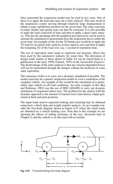
The input loads used to represent braking and cornering may be obtained<br />
using basic vehicle data and weight transfer analysis. As an example consider<br />
the free-body diagram shown in Figure 4.47 where the wheel loads<br />
are obtained for a vehicle braking case. Note that in this example we are<br />
ignoring the effects of rolling resistance in the tyre, discussed later in<br />
Chapter 5, and the vehicle is on flat road with no incline.<br />
cm<br />
mA x<br />
Z<br />
A<br />
mg<br />
B<br />
h<br />
X<br />
F Fx<br />
F Rx<br />
Fig. 4.47<br />
F Fz F SFz F B<br />
a<br />
L<br />
Forward braking free-body diagram<br />
b<br />
F Rz F SRz F B


