chapter - Atmospheric and Oceanic Science

Statistical analysis of extreme events in a non-stationary context
Parametric methods, on the other hand, require specific assumptions about the form
of the underlying probability distribution of the data, and about the form (linear,
curvilinear, etc.) of any trend that may exist. This might seem to be a disadvantage.
However, by assuming a particular probability distribution (provided it is supported
by the data!) it is possible to make inferences about the trend, such as setting limits
to its magnitude, estimating the uncertainty of future values where the user is
sufficiently courageous to extrapolate the trends for a few years ahead; and to test
whether simpler or more complex probability distributions are needed to represent
the data. Thus, despite the fact that they require more assumptions, parametric
methods are generally held to offer a more flexible approach to the study of
extremes, than non-parametric methods. The emphasis in the present report is therefore
on parametric methods. There is now an extensive literature on such methods
(see, for example, the book by Coles 2001, which lists software in S-Plus that can
be downloaded); much material is also available from the internet (see, for example,
the site www.maths.lancs.ac.uk/~stephena/software.html). There is also a journal
(Extremes, published by Kuyper) specifically devoted to developments in the
analysis of extreme values. The book by Coles (2001) has a chapter on the estimation
of trends in the parameters of probability distributions, including the Block
approach used with a Generalized Extreme Value (GEV) probability distribution,
and the POT approach used with exceedances above the threshold represented by a
Generalized Pareto distribution.
15.3. Example: Testing for trend in annual maximum one-hour rainfall at
Porto Alegre, Brazil
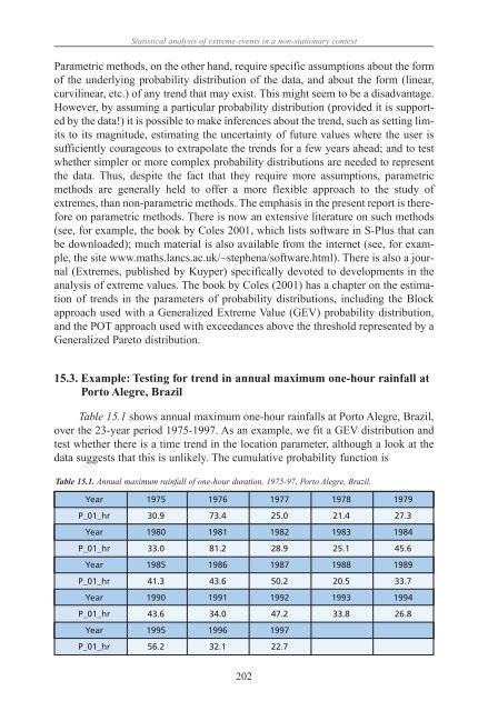
Table 15.1 shows annual maximum one-hour rainfalls at Porto Alegre, Brazil,
over the 23-year period 1975-1997. As an example, we fit a GEV distribution and
test whether there is a time trend in the location parameter, although a look at the
data suggests that this is unlikely. The cumulative probability function is
Table 15.1. Annual maximum rainfall of one-hour duration, 1975-97, Porto Alegre, Brazil.
Year 1975 1976 1977 1978 1979
P_01_hr 30.9 73.4 25.0 21.4 27.3
Year 1980 1981 1982 1983 1984
P_01_hr 33.0 81.2 28.9 25.1 45.6
Year 1985 1986 1987 1988 1989
P_01_hr 41.3 43.6 50.2 20.5 33.7
Year 1990 1991 1992 1993 1994
P_01_hr 43.6 34.0 47.2 33.8 26.8
Year 1995 1996 1997
P_01_hr 56.2 32.1 22.7
202