chapter - Atmospheric and Oceanic Science
chapter - Atmospheric and Oceanic Science
chapter - Atmospheric and Oceanic Science

Create successful ePaper yourself
Turn your PDF publications into a flip-book with our unique Google optimized e-Paper software.
Global climate models<br />
Mid-1970’s Mid-1980’s Early 1990’s Late 1990’s Present day Early 2000’s?<br />
Atmosphere<br />
Atmosphere<br />
L<strong>and</strong><br />
surface<br />
Ocean &<br />
sea-ice<br />
model<br />
Atmosphere<br />
L<strong>and</strong><br />
surface<br />
Ocean &<br />
sea-ice<br />
Sulphur<br />
cycle mode<br />
L<strong>and</strong> carbon<br />
cycle model<br />
Ocean carbon<br />
cycle model<br />
Atmosphere<br />
chemistry<br />
Atmosphere<br />
L<strong>and</strong><br />
surface<br />
Ocean &<br />
sea-ice<br />
Sulphate<br />
aerosol<br />
Non-sulphate<br />
aerosols<br />
Carbon<br />
cycle model<br />
Dynamic<br />
vegetation<br />
Atmosphere<br />
chemistry<br />
11. 2. <strong>Atmospheric</strong> General Circulation Models (AGCMs)<br />
Zero-, one- <strong>and</strong> two-dimensional climate models present a qualitative picture<br />
of how the atmospheric climate system works. However, these models either neglect<br />
various processes that are known to be important in the atmosphere, or they use<br />
simple mathematical representations for these atmospheric process. The representation<br />
of these processes is called parameterization. In order to accurately account<br />
for the general motions of the atmosphere requires the solution of a complete set of<br />
equations. The solution of these equations on the sphere, given realistic boundary<br />
conditions, defines the AGCM (Trenberth 1993).<br />
An AGCM to be implemented requires: a numerical solution technique, algorithms<br />
for the various physical parameterizations, <strong>and</strong> boundary data sets for predetermined<br />
vertical <strong>and</strong> horizontal resolutions. The solution of the system of equations<br />
(called primitive) <strong>and</strong> parameterizations proceeds is outlined in figure 11.2.<br />
Assuming initial data are available for the prognostic variables, the model calculates<br />
initial fluxes for use in the planetary boundary layer (PBL) <strong>and</strong> surface components<br />
of the model. These, along with the thermodynamic <strong>and</strong> moisture profiles<br />
at each gridpoint, are used to test whether the atmospheric column is stable or<br />
unstable. If unstable, a convection parameterization is used to determine the convective<br />
heating <strong>and</strong> moistening terms. Otherwise, if saturated, the stable condensa-<br />
142<br />
Atmosphere<br />
L<strong>and</strong><br />
surface<br />
Ocean &<br />
sea-ice<br />
Sulphate<br />
aerosol<br />
Non-ulphate<br />
aerosol<br />
Carbon<br />
cycle<br />
Dynamic<br />
vegetation<br />
Atmosphere<br />
chemistry<br />
Atmosphere<br />
L<strong>and</strong><br />
surface<br />
Ocean &<br />
sea-ice<br />
Sulphate<br />
aerosol<br />
Non-ulphate<br />
aerosol<br />
Carbon<br />
cycle<br />
Dynamic<br />
vegetation<br />
Atmosphere<br />
chemistry<br />
Fig. 11.1.<br />
Development of climate<br />
models over the last 25<br />
years showing how the<br />
different components<br />
were first developed<br />
separately <strong>and</strong> later<br />
coupled into<br />
comprehensive climate<br />
models.<br />
[Source: IPCC 2001]