Lectures on Quantum Optics and Quantum Information
Lectures on Quantum Optics and Quantum Information
Lectures on Quantum Optics and Quantum Information

Create successful ePaper yourself
Turn your PDF publications into a flip-book with our unique Google optimized e-Paper software.
<str<strong>on</strong>g>Lectures</str<strong>on</strong>g> <strong>on</strong><br />
<strong>Quantum</strong> <strong>Optics</strong> <strong>and</strong><br />
<strong>Quantum</strong> Informati<strong>on</strong><br />
Julien Laurat<br />
Laboratoire Kastler Brossel, Paris<br />
Université P. et M. Curie<br />
Ecole Normale Supérieure <strong>and</strong> CNRS<br />
julien.laurat@upmc.fr<br />
Taiwan-France joint school, Nantou, May 2011
<strong>Quantum</strong> Informati<strong>on</strong> Science<br />
Over the last 20 years, QIS has developed driven by the prospect to<br />
exploit capabilities from the quantum realm to accomplish tasks<br />
difficult or even impossible with traditi<strong>on</strong>al methods of informati<strong>on</strong><br />
processing.<br />
<strong>Quantum</strong> communicati<strong>on</strong>, the art of transferring a quantum state<br />
from <strong>on</strong>e place to another. It led for instance to the dem<strong>on</strong>strati<strong>on</strong> of<br />
quantum cryptography, an absolutely secure way to transmit<br />
informati<strong>on</strong>, <strong>and</strong> even to commercially available quantum key<br />
distributi<strong>on</strong> systems <strong>and</strong> a network deployed in a metropolitan area.<br />
<strong>Quantum</strong> computati<strong>on</strong>, where bits are replaced by qubits. It<br />
detains the promise of computing power bey<strong>on</strong>d the capabilities of<br />
any classical computer. For instance, P. Shor showed that a quantum<br />
computer can factorize a large number efficiently, i.e. in a polynomial<br />
time, while it is an exp<strong>on</strong>entially difficult problem for classical<br />
algorithms. Bey<strong>on</strong>d its fundamental interest for underst<strong>and</strong>ing<br />
quantum complexity, it is of practical importance as the difficulty of<br />
factoring numbers is the basis of encrypti<strong>on</strong> systems, such as the RSA<br />
scheme.<br />
A third directi<strong>on</strong> is quantum metrology <strong>and</strong> enhanced sensing.<br />
M.A. Nielsen, L. Chuang, <strong>Quantum</strong> computati<strong>on</strong> <strong>and</strong> <strong>Quantum</strong> Informati<strong>on</strong>,<br />
Cambridge Univ. Press<br />
S.M. Barnett, <strong>Quantum</strong> Informati<strong>on</strong>, Oxford Univ. Press<br />
H.A. Bachor,T.C. Ralph, A guide to experiments in quantum optics, Wiley-VCH
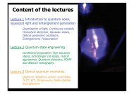
C<strong>on</strong>tent of the lectures<br />
Lecture 1 Introducti<strong>on</strong> to quantum noise,<br />
squeezed light <strong>and</strong> entanglement generati<strong>on</strong><br />
Quantizati<strong>on</strong> of light, C<strong>on</strong>tinuous-variable,<br />
Homodyne detecti<strong>on</strong>, Gaussian states,<br />
Optical parametric oscillators,<br />
Entanglement, Teleportati<strong>on</strong><br />
Lecture 2 <strong>Quantum</strong> state engineering<br />
C<strong>on</strong>diti<strong>on</strong>al preparati<strong>on</strong>, N<strong>on</strong>-Gaussian<br />
states, Schrödinger cat states, Hybrid<br />
approaches, <strong>Quantum</strong> detectors, POVM<br />
<strong>and</strong> detector tomography<br />
Lecture 3 Optical quantum memories.<br />
<strong>Quantum</strong> repeaters, atomic ensembles,<br />
DLCZ, EIT, Phot<strong>on</strong>-echo, Matter-Matter<br />
entanglement
Lecture 1<br />
<strong>Quantum</strong> noise,<br />
squeezed light <strong>and</strong><br />
entanglement<br />
generati<strong>on</strong><br />
Julien Laurat<br />
Laboratoire Kastler Brossel, Paris<br />
Université P. et M. Curie<br />
Ecole Normale Supérieure <strong>and</strong> CNRS<br />
julien.laurat@upmc.fr<br />
Taiwan-France joint school, Nantou, May 2011
Lecture 1<br />
• Light quantizati<strong>on</strong>, discrete vs<br />
c<strong>on</strong>tinuous representati<strong>on</strong><br />
• Measuring <strong>and</strong> characterizing<br />
optical c<strong>on</strong>tinuous variables<br />
• How to generate squeezed light ?<br />
• <strong>Quantum</strong> correlati<strong>on</strong>s <strong>and</strong><br />
entanglement in the CV regime
What Are We Speaking About ?<br />
An introductive example : noise in a light beam<br />
Light<br />
Detector<br />
Scope<br />
Range<br />
In this lecture, we will focus <strong>on</strong><br />
informati<strong>on</strong> carried by travelling light fields<br />
<strong>and</strong> we wil be interested in the<br />
quantum mechanical nature of light.<br />
In the limit of unity<br />
quantum efficiency <strong>and</strong> no<br />
electric noise, the measured<br />
fluctuati<strong>on</strong>s are <strong>on</strong>ly due to<br />
the noise of the light:<br />
it can be classical noise<br />
(e.g. 1/f noise) or quantum<br />
noise (e.g. shot noise).
Quantizati<strong>on</strong> of the Electromagnetic Field<br />
We are not going to detail the quantizati<strong>on</strong> procedure for the free<br />
electromagnetic field, but give here the basic steps <strong>and</strong> analogies,<br />
which enable to introduce useful notati<strong>on</strong>s.<br />
More details can be found for instance in ”Introducti<strong>on</strong> to QO”.<br />
• Maxwell equati<strong>on</strong>s in vacuum (no charges, no currents)<br />
• Give the Helmholtz equati<strong>on</strong> for the E field:<br />
• Classical Plane wave decompositi<strong>on</strong> (l: 2 polarizati<strong>on</strong>s, k: wave vector)<br />
• By injecting this decompositi<strong>on</strong> into the Helmholtz equati<strong>on</strong> :
Quantizati<strong>on</strong> of the Electromagnetic Field<br />
• For each wave vector:<br />
This equati<strong>on</strong> is similar to the <strong>on</strong>e describing the evoluti<strong>on</strong> of a<br />
harm<strong>on</strong>ic oscillator with frequency , which can be described<br />
by a vector a, functi<strong>on</strong> of p (positi<strong>on</strong>) <strong>and</strong> q (momentum).<br />
• By analogy, we introduce an operator a<br />
<strong>and</strong> define a field operator :<br />
We can also define the quadrature operators:<br />
Where <strong>and</strong> can be identified to<br />
the creati<strong>on</strong> <strong>and</strong> annihilati<strong>on</strong> operators for<br />
harm<strong>on</strong>ic oscillators<br />
• By c<strong>on</strong>sidering Fourier-limited wavepackets, it can be shown finally for <strong>on</strong>e mode<br />
(<strong>on</strong>e dimensi<strong>on</strong> quantized harm<strong>on</strong>ic oscillator) :<br />
Total number<br />
of phot<strong>on</strong>s
Two Possible Descripti<strong>on</strong>s<br />
Quantizati<strong>on</strong> of the electromagnetic field<br />
Modes are quantized harm<strong>on</strong>ic oscillators<br />
2 possible observables for the descripti<strong>on</strong>:<br />
Energy or Electric field<br />
Discrete degree of freedom<br />
number of phot<strong>on</strong>s N=a + a<br />
(measured by phot<strong>on</strong> counting)<br />
C<strong>on</strong>tinuous degree of freedom<br />
quadratures P <strong>and</strong> Q<br />
(fluctuati<strong>on</strong>s measured by<br />
homodyning, photodiodes)
Quantizati<strong>on</strong> of the electromagnetic field<br />
Modes are quantized harm<strong>on</strong>ic oscillators<br />
2 possible observables for the descripti<strong>on</strong>:<br />
Energy or Electric field<br />
Discrete Variables<br />
<strong>Quantum</strong> bits or “qu-bits” have been<br />
introduced in this descripti<strong>on</strong>.<br />
e.g. presence/absence of a phot<strong>on</strong> in <strong>on</strong>e<br />
mode, orthog<strong>on</strong>al polarizati<strong>on</strong> modes (H/V),…<br />
A c<strong>on</strong>venient tool : the density matrix<br />
For a pure state:<br />
For a mixed state:<br />
Example :<br />
Discrete degree of freedom<br />
number of phot<strong>on</strong>s N=a + a<br />
(measured by phot<strong>on</strong> counting)<br />
C<strong>on</strong>tinuous degree of freedom<br />
quadratures P <strong>and</strong> Q<br />
(fluctuati<strong>on</strong>s measured by<br />
homodyning, photodiodes)<br />
Written in the Fock basis, the density matrix is very illustrative for discrete systems.
<strong>Quantum</strong> C<strong>on</strong>tinuous-Variables<br />
Quantizati<strong>on</strong> of the electromagnetic field<br />
Modes are quantized harm<strong>on</strong>ic oscillators<br />
2 possible observables for the descripti<strong>on</strong>:<br />
Energy or Electric field<br />
Discrete degree of freedom<br />
number of phot<strong>on</strong>s N=a + a<br />
(measured by phot<strong>on</strong> counting)<br />
C<strong>on</strong>tinuous degree of freedom<br />
quadratures P <strong>and</strong> Q<br />
(fluctuati<strong>on</strong>s measured by<br />
homodyning, photodiodes)<br />
Why using them?<br />
- Perfect detectors, high<br />
rates/b<strong>and</strong>width<br />
- Deterministic operati<strong>on</strong>s<br />
- N<strong>on</strong>-gaussian states/cluster<br />
states with many potential<br />
applicati<strong>on</strong>s in Q. computing<br />
<strong>and</strong> communicati<strong>on</strong>
<strong>Quantum</strong> C<strong>on</strong>tinuous-Variables<br />
Quantizati<strong>on</strong> of the electromagnetic field<br />
Modes are quantized harm<strong>on</strong>ic oscillators<br />
2 possible observables for the descripti<strong>on</strong>:<br />
Energy or Electric field<br />
Q A<br />
Q<br />
Amplitude<br />
Fresnel Diagram for the Electromagnetic Field<br />
Phase<br />
P A<br />
P<br />
Discrete degree of freedom<br />
number of phot<strong>on</strong>s N=a + a<br />
(measured by phot<strong>on</strong> counting)<br />
C<strong>on</strong>tinuous degree of freedom<br />
quadratures P <strong>and</strong> Q<br />
(fluctuati<strong>on</strong>s measured by<br />
homodyning, photodiodes)<br />
Why using them?<br />
- Perfect detectors, high<br />
rates/b<strong>and</strong>width<br />
- Deterministic operati<strong>on</strong>s<br />
- N<strong>on</strong>-gaussian states/cluster<br />
states with many potential<br />
applicati<strong>on</strong>s in Q. computing<br />
<strong>and</strong> communicati<strong>on</strong>
Q A<br />
Q<br />
<strong>Quantum</strong> C<strong>on</strong>tinuous-Variables<br />
Quantizati<strong>on</strong> of the electromagnetic field<br />
Modes are quantized harm<strong>on</strong>ic oscillators<br />
2 possible observables for the descripti<strong>on</strong>:<br />
Energy or Electric field<br />
P A<br />
Fano factor F<br />
P<br />
Phasor Diagram<br />
Discrete degree of freedom<br />
number of phot<strong>on</strong>s N=a + a<br />
(measured by phot<strong>on</strong> counting)<br />
C<strong>on</strong>tinuous degree of freedom<br />
quadratures P <strong>and</strong> Q<br />
(fluctuati<strong>on</strong>s measured by<br />
homodyning, photodiodes)<br />
Why using them?<br />
- Perfect detectors, high<br />
rates/b<strong>and</strong>width<br />
- Deterministic operati<strong>on</strong>s<br />
- N<strong>on</strong>-gaussian states/cluster<br />
states with many potential<br />
applicati<strong>on</strong>s in Q. computing<br />
<strong>and</strong> communicati<strong>on</strong>
Q A<br />
Q<br />
<strong>Quantum</strong> C<strong>on</strong>tinuous-Variables<br />
Quantizati<strong>on</strong> of the electromagnetic field<br />
Modes are quantized harm<strong>on</strong>ic oscillators<br />
2 possible observables for the descripti<strong>on</strong>:<br />
Energy or Electric field<br />
P A<br />
P<br />
Squeezing<br />
One can have :<br />
“Noise<br />
reducti<strong>on</strong>”<br />
or “Squeezing”<br />
Discrete degree of freedom<br />
number of phot<strong>on</strong>s N=a + a<br />
(measured by phot<strong>on</strong> counting)<br />
C<strong>on</strong>tinuous degree of freedom<br />
quadratures P <strong>and</strong> Q<br />
(fluctuati<strong>on</strong>s measured by<br />
homodyning, photodiodes)<br />
Why using them?<br />
- Perfect detectors, high<br />
rates/b<strong>and</strong>width<br />
- Deterministic operati<strong>on</strong>s<br />
- N<strong>on</strong>-gaussian states/cluster<br />
states with many potential<br />
applicati<strong>on</strong>s in Q. computing<br />
<strong>and</strong> communicati<strong>on</strong>
<strong>Quantum</strong> C<strong>on</strong>tinuous-Variables<br />
Quantizati<strong>on</strong> of the electromagnetic field<br />
Modes are quantized harm<strong>on</strong>ic oscillators<br />
2 possible observables for the descripti<strong>on</strong>:<br />
Energy or Electric field<br />
1<br />
Coherent state<br />
Vacuum<br />
Number state<br />
Intensity squeezing<br />
Squeezed Vacuum<br />
Zoology of states<br />
Gaussian<br />
states<br />
N<strong>on</strong>-Gaussian<br />
states<br />
Discrete degree of freedom<br />
number of phot<strong>on</strong>s N=a + a<br />
(measured by phot<strong>on</strong> counting)<br />
C<strong>on</strong>tinuous degree of freedom<br />
quadratures P <strong>and</strong> Q<br />
(fluctuati<strong>on</strong>s measured by<br />
homodyning, photodiodes)<br />
Why using them?<br />
- Perfect detectors, high<br />
rates/b<strong>and</strong>width<br />
- Deterministic operati<strong>on</strong>s<br />
- N<strong>on</strong>-gaussian states/cluster<br />
states with many potential<br />
applicati<strong>on</strong>s in Q. computing<br />
<strong>and</strong> communicati<strong>on</strong>
Lecture 1<br />
• Light quantizati<strong>on</strong>, discrete vs<br />
c<strong>on</strong>tinuous representati<strong>on</strong><br />
• Measuring <strong>and</strong> characterizing<br />
optical c<strong>on</strong>tinuous variables<br />
• How to generate squeezed light ?<br />
• <strong>Quantum</strong> correlati<strong>on</strong>s <strong>and</strong><br />
entanglement in the CV regime
Measuring Optical C<strong>on</strong>tinuous-Variables<br />
THE tool : Homodyne detecti<strong>on</strong><br />
<strong>Quantum</strong> state<br />
50/50<br />
Photocurrent<br />
subtracti<strong>on</strong><br />
Local oscillator<br />
Adjustable Phase<br />
Local oscillator
Measuring Optical C<strong>on</strong>tinuous-Variables<br />
THE tool : Homodyne detecti<strong>on</strong><br />
<strong>Quantum</strong> state<br />
50/50<br />
Photocurrent<br />
subtracti<strong>on</strong><br />
Local oscillator<br />
Adjustable Phase<br />
• Annihilati<strong>on</strong> operators of the mixed modes:<br />
• After subtracti<strong>on</strong>, the resulting photocurrent operator is:<br />
• Mean Value <strong>and</strong> variance for :<br />
Local oscillator<br />
For large phot<strong>on</strong> number in lo:
Measuring Optical C<strong>on</strong>tinuous-Variables<br />
THE tool : Homodyne detecti<strong>on</strong><br />
<strong>Quantum</strong> state<br />
50/50<br />
Photocurrent<br />
subtracti<strong>on</strong><br />
Local oscillator<br />
Adjustable Phase<br />
• Annihilati<strong>on</strong> operators of the mixed modes:<br />
• After subtracti<strong>on</strong>, the resulting photocurrent operator is:<br />
• Mean Value <strong>and</strong> variance for :<br />
Local oscillator<br />
- Overall Efficiency -<br />
Photodiode efficiency<br />
Interference Visibility V<br />
tot = .V2<br />
(ex: 0.99 x 0.992 =0.97)<br />
For large phot<strong>on</strong> number in lo:
Measuring Optical C<strong>on</strong>tinuous-Variables<br />
THE tool : Homodyne detecti<strong>on</strong><br />
<strong>Quantum</strong> state<br />
What we obtain ? Example of a squeezed state<br />
Photocurrent <strong>Quantum</strong> state<br />
Phase<br />
50/50<br />
Photocurrent<br />
subtracti<strong>on</strong><br />
Local oscillator<br />
Adjustable Phase<br />
Local oscillator<br />
- Overall Efficiency -<br />
Photodiode efficiency<br />
Interference Visibility V<br />
tot = .V2<br />
(ex: 0.99 x 0.992 =0.97)<br />
Probability distributi<strong>on</strong> P (X, ) Variance<br />
TF : Noise spectrum
The Wigner Functi<strong>on</strong><br />
For c<strong>on</strong>tinuous-variable, the density matrix is useful, but not easy to interpret.<br />
Another tool : the Wigner functi<strong>on</strong>, which is a quasi-probability distributi<strong>on</strong>.<br />
Marginal distributi<strong>on</strong>s for (what is measured with homodyne detecti<strong>on</strong>) are<br />
obtained by projecti<strong>on</strong> of the Wigner functi<strong>on</strong> <strong>on</strong> the axis defined by , i.e. by<br />
integrating it over the orthog<strong>on</strong>al directi<strong>on</strong>.<br />
Importantly, <strong>on</strong>e can also obtain <strong>and</strong> W from the marginal distributi<strong>on</strong>s : this is the<br />
goal of tomography. It requires to use rec<strong>on</strong>structi<strong>on</strong> algorithm, such as Rad<strong>on</strong><br />
transform or Maximum-likelihood algorithm. [see A.Lvovsky, RMP 81, 299 (2009)]<br />
Wigner functi<strong>on</strong><br />
<strong>and</strong> some<br />
projecti<strong>on</strong>s for a<br />
squeezed state<br />
From A. Ourjoumtsev PhD Thesis
The Wigner Functi<strong>on</strong>: Functi<strong>on</strong>:<br />
Negativity<br />
(From A. Ourjoumtsev PhD Thesis)<br />
Wigner functi<strong>on</strong> of<br />
a single-phot<strong>on</strong><br />
The Wigner functi<strong>on</strong> is a quasi-probability<br />
distributi<strong>on</strong>: it can take negative values.<br />
Huds<strong>on</strong>-Piquet Theorem for pure state:<br />
Gaussian state Positive Wigner functi<strong>on</strong><br />
N<strong>on</strong>-Gaussian state Negative Wigner functi<strong>on</strong>
The Wigner Functi<strong>on</strong>: Functi<strong>on</strong>:<br />
Negativity<br />
(From A. Ourjoumtsev PhD Thesis)<br />
Wigner functi<strong>on</strong> of<br />
a single-phot<strong>on</strong><br />
The Wigner functi<strong>on</strong> is a quasi-probability<br />
distributi<strong>on</strong>: it can take negative values.<br />
Huds<strong>on</strong>-Piquet Theorem for pure state:<br />
Gaussian state Positive Wigner functi<strong>on</strong><br />
N<strong>on</strong>-Gaussian state Negative Wigner functi<strong>on</strong><br />
Negativity at the origin, W(0,0)
Measuring Optical CV : a Summary<br />
Squeezed Vacuum<br />
(or other <strong>Quantum</strong> states!) state<br />
Density matrix<br />
Homodyne detecti<strong>on</strong><br />
50/50<br />
Photocurrent<br />
subtracti<strong>on</strong><br />
Local oscillator<br />
Adjustable Phase<br />
Photocurrent vs phase<br />
Give the marginal distributi<strong>on</strong>s<br />
By rec<strong>on</strong>structi<strong>on</strong> algorithm (Rad<strong>on</strong>, MaxLik) Variance, Fourier Transform<br />
Wigner functi<strong>on</strong><br />
Noise spectrum
Interlude: CV for Atomic Ensembles<br />
N 2-level atoms<br />
N fictitious 1/2 spins described<br />
by a collective spin<br />
Collective spin operators<br />
Individual spins aligned al<strong>on</strong>g Oz<br />
Heisenberg inequality
Interlude: CV for Atomic Ensembles<br />
N 2-level atoms<br />
N fictitious 1/2 spins described<br />
by a collective spin<br />
Some atomic states…<br />
Collective spin operators<br />
Individual spins aligned al<strong>on</strong>g Oz<br />
Heisenberg inequality<br />
Uncorrelated spins Correlated spins<br />
Spin coherent state Spin squeezed state
Lecture 1<br />
• Light quantizati<strong>on</strong>, discrete vs<br />
c<strong>on</strong>tinuous representati<strong>on</strong><br />
• Measuring <strong>and</strong> characterizing<br />
optical c<strong>on</strong>tinuous variables<br />
• How to generate squeezed light ?<br />
• <strong>Quantum</strong> correlati<strong>on</strong>s <strong>and</strong><br />
entanglement in the CV regime
How to Generate Squeezed Light ?<br />
Squeezed light generati<strong>on</strong> requires the use<br />
of n<strong>on</strong>-linear effects. We focus here <strong>on</strong> the<br />
case of degenerate parametric interacti<strong>on</strong> in<br />
n<strong>on</strong>-linear (2) crystals.<br />
pump<br />
signal<br />
idler<br />
‘Degenerate’: signal <strong>and</strong> idler<br />
identical (frequency, polarizati<strong>on</strong>)
How to Generate Squeezed Light ?<br />
Squeezed light generati<strong>on</strong> requires the use<br />
of n<strong>on</strong>-linear effects. We focus here <strong>on</strong> the<br />
case of degenerate parametric interacti<strong>on</strong> in<br />
n<strong>on</strong>-linear (2) crystals.<br />
pump<br />
signal<br />
idler<br />
‘Degenerate’: signal <strong>and</strong> idler<br />
identical (frequency, polarizati<strong>on</strong>)<br />
• Hamilt<strong>on</strong>ian associated to this process (down c<strong>on</strong>versi<strong>on</strong> <strong>and</strong> up c<strong>on</strong>versi<strong>on</strong>):<br />
• It leads to the temporal evoluti<strong>on</strong><br />
• This gives for the quadratures after the interacti<strong>on</strong> :<br />
One quadrature is amplified while the<br />
orthog<strong>on</strong>al <strong>on</strong>e is deamplified.<br />
Degenerate case
Pulsed Parametric Amplificati<strong>on</strong><br />
Requires intense pulses.<br />
Squeezing increases with<br />
pump power.<br />
Opt. p Lett. 29, 1267 (2004)
CW Parametric Amplificati<strong>on</strong> in a Cavity<br />
Another soluti<strong>on</strong>: use a cw less<br />
intense pump laser <strong>and</strong> a cavity<br />
which is res<strong>on</strong>ant <strong>on</strong> the comm<strong>on</strong><br />
signal-idler mode <strong>and</strong> enhances the<br />
n<strong>on</strong>-linear interacti<strong>on</strong>.<br />
‘Optical Parametric Oscillator’, which<br />
can oscillate above a given<br />
threshold.<br />
(Output coupler R,T)<br />
- R=1 for all the mirrors, but the output coupler R<br />
- Losses L (absorpti<strong>on</strong>, interfaces,..)<br />
- Pump power normalized to the threshold :<br />
c : cavity b<strong>and</strong>width
CW Parametric Amplificati<strong>on</strong> in a Cavity<br />
Another soluti<strong>on</strong>: use a cw less<br />
intense pump laser <strong>and</strong> a cavity<br />
which is res<strong>on</strong>ant <strong>on</strong> the comm<strong>on</strong><br />
signal-idler mode <strong>and</strong> enhances the<br />
n<strong>on</strong>-linear interacti<strong>on</strong>.<br />
‘Optical Parametric Oscillator’, which<br />
can oscillate above a given<br />
threshold.<br />
Maximum squeezing : at threshold, at<br />
zero frequency.<br />
Squeezing <strong>on</strong>ly depends <strong>on</strong> the<br />
escape efficiency T/(T+L)<br />
Ex. : T=10%, L=1% -->V=1-10/11~0.09 (~10dB)<br />
(Output coupler R,T)<br />
- R=1 for all the mirrors, but the output coupler R<br />
- Losses L (absorpti<strong>on</strong>, interfaces,..)<br />
- Pump power normalized to the threshold :<br />
c : cavity b<strong>and</strong>width
CW Parametric Amplificati<strong>on</strong> in a Cavity<br />
See also works from Paris, Copenhaguen, Tokyo, Naples, Canberra,…<br />
Phys. Rev. A 81, 013814 (2010)<br />
~12 dB of<br />
squeezing (94%)
GW Detecti<strong>on</strong> <strong>and</strong> <strong>Quantum</strong> Imaging<br />
Class.Quant.Grav.27:084027 (2010)<br />
Science 301, 940 (2003)
Effect of Losses <strong>on</strong> Squeezed Light<br />
Model of losses in quantum optics<br />
Intensity loss : 1-<br />
Can be modelled by a beam<br />
splitter with reflectivity R=1<strong>and</strong><br />
transmitivity T= .<br />
Vacuum fluctuati<strong>on</strong>s are<br />
entering by the empty port.<br />
What is<br />
the noise<br />
after the<br />
loss?
Effect of Losses <strong>on</strong> Squeezed Light<br />
Model of losses in quantum optics<br />
Intensity loss : 1-<br />
Can be modelled by a beam<br />
splitter with reflectivity R=1<strong>and</strong><br />
transmitivity T= .<br />
Vacuum fluctuati<strong>on</strong>s are<br />
entering by the empty port.<br />
Calculati<strong>on</strong>s<br />
• We linearize the fluctuati<strong>on</strong>s :<br />
<strong>and</strong> obtain for a quadrature P:<br />
• We calculate the noise variance :<br />
=V’<br />
• The beam-splitter gives:<br />
=V<br />
=1 (shot)<br />
What is<br />
the noise<br />
after the<br />
loss?<br />
<strong>and</strong><br />
V’ goes to 1 (shot) for str<strong>on</strong>g losses ( =0), ok!<br />
=0 (uncorrelated)
Effect of Losses <strong>on</strong> Squeezed Light<br />
Model of losses in quantum optics<br />
Intensity loss : 1-<br />
Can be modelled by a beam<br />
splitter with reflectivity R=1<strong>and</strong><br />
transmitivity T= .<br />
Vacuum fluctuati<strong>on</strong>s are<br />
entering by the empty port.<br />
Calculati<strong>on</strong>s<br />
• We linearize the fluctuati<strong>on</strong>s :<br />
<strong>and</strong> obtain for a quadrature P:<br />
• We calculate the noise variance :<br />
=V’<br />
• The beam-splitter gives:<br />
=V<br />
=1 (shot)<br />
What is<br />
the noise<br />
after the<br />
loss?<br />
<strong>and</strong><br />
V’ goes to 1 (shot) for str<strong>on</strong>g losses ( =0), ok!<br />
Some illlustrative values…..<br />
V=0.1 (10dB squeezing)<br />
10% loss give:<br />
V’=0.2 (7dB squeezing)<br />
Squeezing is very<br />
sensitive to losses!<br />
=0 (uncorrelated)
Lecture 1<br />
• Light quantizati<strong>on</strong>, discrete vs<br />
c<strong>on</strong>tinuous representati<strong>on</strong><br />
• Measuring <strong>and</strong> characterizing<br />
optical c<strong>on</strong>tinuous variables<br />
• How to generate squeezed light ?<br />
• <strong>Quantum</strong> correlati<strong>on</strong>s <strong>and</strong><br />
entanglement in the CV regime
Classical Correlati<strong>on</strong>s of Light Beams<br />
A simple example : intensity « correlati<strong>on</strong>s » is easy to obtain….<br />
Linear Correlati<strong>on</strong> coefficient<br />
For a very noisy incident beam, the<br />
correlati<strong>on</strong> goes to 1!
Classical Correlati<strong>on</strong>s of Light Beams<br />
A simple example : intensity « correlati<strong>on</strong>s » is easy to obtain….<br />
Questi<strong>on</strong> : How to define the quantum character of<br />
correlati<strong>on</strong>s between two beams in the CV regime?<br />
Involving 1 quadrature<br />
Gemellity<br />
QND Correlati<strong>on</strong><br />
Normalized linear correlati<strong>on</strong> coefficient<br />
For a very noisy incident beam, the<br />
correlati<strong>on</strong> goes to 1 !<br />
Involving 2 quadratures<br />
Inseparability<br />
EPR Correlati<strong>on</strong>s
« One Quadrature » Criteria<br />
Two beams, <strong>on</strong>e quadature<br />
Q<br />
Q<br />
Field 1 Field 2<br />
P<br />
- Difference between the fluctuati<strong>on</strong>s<br />
- Noise <strong>on</strong> this difference<br />
G=1 for two independent lasers (also<br />
for the previous case with noisy beam)<br />
- C<strong>on</strong>diti<strong>on</strong>al Variance V(P 1 |P 2 )<br />
P
« One Quadrature » Criteria<br />
Two beams, <strong>on</strong>e quadature<br />
Q<br />
Q<br />
Field 1 Field 2<br />
P<br />
- Difference between the fluctuati<strong>on</strong>s<br />
- Noise <strong>on</strong> this difference<br />
G=1 for two independent lasers (also<br />
for the previous case with noisy beam)<br />
- C<strong>on</strong>diti<strong>on</strong>al Variance V(P 1 |P 2 )<br />
P<br />
Gemellity : G
<strong>Quantum</strong> Intensity Correlati<strong>on</strong>s<br />
With a type-II optical parametric oscillator<br />
Optical Cavity<br />
CW Pump<br />
NL Crystal (2)<br />
Type-II Phase matching<br />
Signal H<br />
<strong>and</strong> Idler V<br />
Noise <strong>on</strong> the intensity<br />
difference ?<br />
J. Laurat et al., Phys. Rev. Lett 91, 213601 (2003); <strong>Optics</strong> Lett. 30, 1177 (2005); arXiv:quant-ph/0510063
<strong>Quantum</strong> Intensity Correlati<strong>on</strong>s<br />
With a type-II optical parametric oscillator<br />
Optical Cavity<br />
CW Pump<br />
NL Crystal (2)<br />
Type-II Phase matching<br />
G=0.11
« Two Quadratures » Criteria<br />
A double correlati<strong>on</strong> : « EPR Paradox »<br />
Phys. Rev. 47, 777 (1935)
« Two Quadratures » Criteria<br />
A double correlati<strong>on</strong> : « EPR Paradox »<br />
Inseparabilty (Duan) :
« Two Quadratures » Criteria<br />
A double correlati<strong>on</strong> : « EPR Paradox »<br />
Inseparabilty (Duan) :
How to Generate CV Entanglement ?<br />
Entanglement <strong>and</strong> Squeezing : a change in basis<br />
-Using 2 type-I OPO <strong>and</strong><br />
mixing the two squeezed<br />
light <strong>on</strong> BS<br />
- Using 1 type II OPO
How to Generate CV Entanglement ?<br />
Entanglement <strong>and</strong> Squeezing : a change in basis<br />
J. Laurat et al., Phys. Rev. A 71, 022313 (2005)<br />
Separability = 0.33 ± 0.02 < 1<br />
EPR: Vc 1 .Vc 2 = 0.42 ± 0.05
How to Generate CV Entanglement ?<br />
With <strong>on</strong>e squeezed beam?<br />
Squeezing s1<br />
?
How to Generate CV Entanglement ?<br />
With <strong>on</strong>e squeezed beam?<br />
Squeezing s1<br />
?<br />
Always entangled…<br />
Sometimes EPR entangled : needs good<br />
squeezing <strong>and</strong> importantly good purity
How to Generate CV Entanglement ?<br />
With <strong>on</strong>e squeezed beam?<br />
Squeezing s1<br />
?<br />
Always entangled…<br />
Sometimes EPR entangled : needs good<br />
squeezing <strong>and</strong> importantly good purity<br />
arXiv:1103.1817
<strong>Quantum</strong> Teleportati<strong>on</strong><br />
1- Measurements<br />
2- Transmissi<strong>on</strong> (classical channel)<br />
3- Modulati<strong>on</strong>s<br />
First teleporati<strong>on</strong> of a coherent states with Fidelity above 0.5 (1/2=classical strategy)<br />
A. Furusawa et al., Unc<strong>on</strong>diti<strong>on</strong>al quantum teleportati<strong>on</strong>, Science 282, 706 (1998)<br />
First teleportati<strong>on</strong> of a cat states<br />
N. Lee et al., Teleportati<strong>on</strong> of n<strong>on</strong>-classical wave-packets of light, Science 332, 330 (2011)<br />
0<br />
0
Multimode Entanglement : Cluster States<br />
CV Cluster states<br />
Quadrature correlati<strong>on</strong>s verifying:
Multimode Entanglement : Cluster States<br />
CV Cluster states<br />
Quadrature correlati<strong>on</strong>s verifying:<br />
How to build them? With squeezers <strong>and</strong> beam splitters<br />
With other phase combinati<strong>on</strong>s:<br />
M. Yukawa et al., Experimental generati<strong>on</strong> of four-modes CV cluster states, Phys. Rev. A 78, 012301 (2008)
A last Level of Correlati<strong>on</strong>s : N<strong>on</strong>-locality<br />
Violati<strong>on</strong> of a Bell Inequality<br />
The multiple correlati<strong>on</strong>s cannot be described by a<br />
local hidden variables<br />
Fields with Gaussian statistics (Positive Wigner<br />
functi<strong>on</strong>) : can always be mapped into<br />
stochastic equati<strong>on</strong>s for fluctuating fields,<br />
which c<strong>on</strong>stitute the local « hidden » variables<br />
accounting for all the observed quantities…<br />
N<strong>on</strong>-Gaussian states with<br />
Negative Wigner functi<strong>on</strong>s<br />
A str<strong>on</strong>gly active field:<br />
Schrodinger cat states,<br />
CV qubit, distillati<strong>on</strong><br />
Hybrid Schemes<br />
Requires n<strong>on</strong>-Gaussian<br />
measurements or n<strong>on</strong>-Gaussian<br />
ressources
A last Level of Correlati<strong>on</strong>s : N<strong>on</strong>-locality<br />
Violati<strong>on</strong> of a Bell Inequality<br />
The multiple correlati<strong>on</strong>s cannot be described by a<br />
local hidden variables<br />
Fields with Gaussian statistics (Positive Wigner<br />
functi<strong>on</strong>) : can always be mapped into<br />
stochastic equati<strong>on</strong>s for fluctuating fields,<br />
which c<strong>on</strong>stitute the local « hidden » variables<br />
accounting for all the observed quantities…<br />
Single-phot<strong>on</strong> subtracti<strong>on</strong>s<br />
N<strong>on</strong>-Gaussian states with<br />
Negative Wigner functi<strong>on</strong>s<br />
A str<strong>on</strong>gly active field:<br />
Schrodinger cat states,<br />
CV qubit, distillati<strong>on</strong><br />
Hybrid Schemes<br />
Requires n<strong>on</strong>-Gaussian<br />
measurements or n<strong>on</strong>-Gaussian<br />
ressources<br />
Requires efficiency>95%, 6dB<br />
squeezing, high-purity of the<br />
initial state…<br />
And gives at most S=2.05<br />
R. Garcia-Patr<strong>on</strong> et al., Phys. Rev. Lett. 93, 130409 (2004); <strong>and</strong> many other proposals since then…
Summary<br />
• C<strong>on</strong>tinuous-variable regime<br />
• Measuring optical CV<br />
• Squezed light generati<strong>on</strong> by<br />
parametric amplificati<strong>on</strong><br />
• <strong>Quantum</strong> correlati<strong>on</strong>s : 5 levels<br />
Gaussian: Twins, QND,EPR<br />
N<strong>on</strong>-Gaussian : Bell-type<br />
Trend: Hybrid schemes (next lecture!)