SPA 3e_ Teachers Edition _ Ch 6

Activity answers continued
3. Yes, this confirms our observations in
Step 2.
4. Students should paint their own
population distribution. Yes, this is
cool. The results from Steps 1 to 3
hold true for this new population (no
matter what the population looks like)!
5. The sampling distribution of x has
the same mean as the population
distribution. As n increases, the
variability in the sampling distribution
decreases. The shape of the
sampling distribution becomes more
approximately normal as n increases.
440
C H A P T E R 6 • Sampling Distributions
The Central Limit Theorem
It is a remarkable fact that as the sample size increases, the sampling distribution
of x changes shape: It looks less like that of the population and more like a normal
distribution. This is true no matter what shape the population distribution has. This
famous fact of probability theory is called the central limit theorem (sometimes abbreviated
as CLT).
DEFINITION central limit theorem (cLt)
Draw an SRS of size n from any population with mean m and finite standard deviation s.
The central limit theorem (CLT) says that when n is large, the sampling distribution of
the sample mean x is approximately normal.
How large a sample size n is needed for the sampling distribution of x to be close
to normal depends on the population distribution. A larger sample size is required
if the shape of the population distribution is far from normal. In that case, the sampling
distribution of x will also be far from normal if the sample size is small. To use
a normal distribution to calculate probabilities involving x, check the Normal/Large
Sample condition.
Teaching Tip
It is hard to overstate the importance
of the central limit theorem. Students
should know this theorem by name.
Make sure students understand that the
CLT applies to sample means and refers
to the shape (and only the shape) of the
sampling distribution of x.
Teaching Tip
There is nothing magical about 30 as
the boundary value for a “large” sample
size. Some statisticians and authors
recommend n 5 40 as the boundary.
In truth, some populations need
sample sizes much larger than 40 to
have sampling distributions that are
approximately normal. For our purposes,
30 is a reasonable value that works
relatively well for most populations.
Make sure that students understand that
n ≥ 30 is just a guideline (like the Large
Counts condition for proportions).
a
e XAMPLe
A few more pennies for your thoughts?
Sampling from a non-normal population
DEFINITION normal/Large Sample condition
The Normal/Large Sample condition says that the distribution of x will be approximately
normal when either of the following is true:
• The population distribution is approximately normal. This is true no matter what the
sample size n is.
• The sample size is large. If the population distribution is not normal, the sampling
distribution of x will be approximately normal in most cases if n ≥ 30.
PROBLEM: Mr. Ramirez’s class did the Penny for Your
Thoughts Activity from the beginning of this chapter.
The histogram shows the distribution of ages for the
2341 pennies in their collection.
(a) Describe the shape of the sampling distribution
of x for SRSs of size n 5 2 from the population of
pennies. Justify your answer.
(b) Describe the shape of the sampling distribution
of x for SRSs of size n 5 50 from the population of
pennies. Justify your answer.
Frequency
140
120
100
80
60
40
20
0
1950 1960 1970 1980 1990 2000 2010 2020
Year
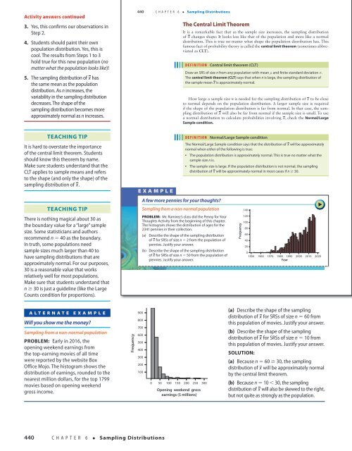
Alternate Example
Will you show me the money?
Sampling from a non-normal population
PROBLEM: Early in 2016, the
opening weekend earnings from
the top-earning movies of all time
were reported by the website Box
Office Mojo. The histogram shows the
distribution of earnings, rounded to the
nearest million dollars, for the top 1799
movies based on opening weekend
gross income.
Starnes_3e_CH06_398-449_Final.indd 440
Frequency
900
800
700
600
500
400
300
200
100
0
50 100 150 200 250 300
Opening weekend gross
earnings ($ millions)
(a) Describe the shape of the sampling
distribution of x for SRSs of size n 5 60 from
this population of movies. Justify your answer.
(b) Describe the shape of the sampling
distribution of x for SRSs of size n 5 10 from
this population of movies. Justify your answer.
SOLUTION:
(a) Because n 5 60 ≥ 30, the sampling
distribution of x will be approximately normal
by the central limit theorem.
(b) Because n 5 10 < 30, the sampling
distribution of x will also be skewed to the right,
but not quite as strongly as the population.
18/08/16 5:03 PMStarnes_3e_CH0
440
C H A P T E R 6 • Sampling Distributions
Starnes_3e_ATE_CH06_398-449_v3.indd 440
11/01/17 3:58 PM