SPA 3e_ Teachers Edition _ Ch 6

More documents

Recommendations

Info

420 C H A P T E R 6 • Sampling Distributions As you learned in the activity, the shape of the sampling distribution of X will be approximately normal when the sample size is large enough. You also learned that “large enough” depends on the value of p. The farther p is from 0.5, the larger the sample size needs to be, as shown in Figure 6.7. 0.330 0.234 0.148 Probability 0.165 Probability 0.117 Probability 0.074 Teaching Tip Make sure students understand that both np and n(1 2 p) must be checked to see if they are at least 10. FYI The Large Counts condition presented here is one rule of thumb for ensuring that a binomial distribution is approximately normal. Another criterion is np ≥ 5 and n(1 2 p) ≥ 5. We recommend the Large Counts condition stated here. 0.000 0 8 10 (a) n = 10, p = 0.8 0.000 0.000 0 16 20 0 40 50 (b) n = 20, p = 0.8 (c) n = 50, p = 0.8 FigUre 6.7 Histograms of the sampling distribution of a sample count X with (a) n 5 10 and p 5 0.8, (b) n 5 20 and p 5 0.8, and (c) n 5 50 and p 5 0.8. As n increases, the shape of the sampling distribution gets closer and closer to normal. In practice, the sampling distribution of a sample count will have an approximately normal distribution when the Large Counts condition is met. DEFINITION the Large counts condition Suppose X is the number of successes in a random sample of size n from a population with proportion of successes p. The Large Counts condition says that the distribution of X will be approximately normal when np ≥ 10 and n(1 2 p) ≥10 This condition is called “large counts” because np is the expected (mean) count of successes and n(1 2 p) is the expected (mean) count of failures. Alternate Example Spend or save? Shape of the sampling distribution of a sample count PROBLEM: Suppose that 24% of all Americans have more debt on their credit cards than they have money in their savings accounts. Let X 5 the number of Americans with more debt than savings in a random sample of 40 Americans. Would it be appropriate to use a normal distribution to model the sampling distribution of X ? Justify your answer. SOLUTION: a e XAMPLe How many teens have debit cards? Shape of the sampling distribution of a sample count PROBLEM: Suppose that 12% of teens in a large city have a debit card. Let X 5 the number of teens with a debit card in a random sample of 500 teens from this city. Would it be appropriate to use a normal distribution to model the sampling distribution of X? Justify your answer. SOLUTION: Because np 5 500(0.12) 5 60 ≥ 10 and n (1 2 p ) 5 500 (1 2 0.12) 5 440 ≥ 10, the sampling distribution of X is approximately normal. Check the Large Counts condition to determine if X will have an approximately normal distribution. In this context, 60 is the expected (mean) count of teens with a debit card and 440 is the expected (mean) count of teens without a debit card. FOR PRACTICE TRY EXERCISE 5. Because np 5 40(0.24) 5 9.6 < 10, the sampling distribution of X is not approximately normal. Although n(1 2 p) 5 40(1 2 0.24) 5 30.4 ≥ 10, we have still not met the Large Counts condition. Starnes_3e_CH06_398-449_Final.indd 420 18/08/16 5:01 PMStarnes_3e_CH0 420 C H A P T E R 6 • Sampling Distributions Starnes_3e_ATE_CH06_398-449_v3.indd 420 11/01/17 3:55 PM
L E S S O N 6.3 • The Sampling Distribution of a Sample Count 421 Finding Probabilities Involving X When the Large Counts condition is met, we can use a normal distribution to calculate probabilities involving X 5 the number of successes in a random sample of size n. Is it fun to shop anymore? Probabilities involving X PROBLEM: Sample surveys show that fewer people enjoy shopping than in the past. A survey asked a nationwide random sample of 2500 adults if they agreed or disagreed with the statement “I like buying new clothes, but shopping is often frustrating and time-consuming.” 5 Suppose that exactly 60% of all adult U.S. residents would say “Agree” if asked the same question. Calculate the probability that at least 1520 members of the sample would say “Agree.” SOLUTION: • Mean: m X 5 2500(0.60) 5 1500 • SD: s X = "2500(0.6)(1 − 0.6) 5 24.49 • Shape: Approximately normal because np 5 2500 (0.60) 5 1500 ≥ 10 and n (1 2 p ) 5 2500 (1 2 0.6) 5 1000 ≥ 10 1426.53 1451.02 1475.51 1500 1524.49 1548.98 1573.47 1520 Sample count who would say “Agree” 1520 − 1500 Using Table A: Z = = 0.82 24.49 P (Z ≥ 0.82) 5 1 2 0.7939 5 0.2061 Using technology : Applet/normalcdf (lower:1520, upper:100000, mean:1500, SD: 24.49) 5 0.2071 e XAMPLe Let X 5 the number who would say “Agree.” The sampling distribution of X is approximately binomial with n 5 2500 and p 5 0.60. To use a normal approximation to calculate probabilities involving X, we need to know the mean, standard deviation, and shape of the sampling distribution of X. Recall that the mean is m X = np and the standard deviation is s X = "np(1 − p). 1. Draw a normal distribution. 2. Perform calculations. (i) Standardize the boundary value and use Table A to find the desired probability; or (ii) Use technology. FOR PRACTICE TRY EXERCISE 9. 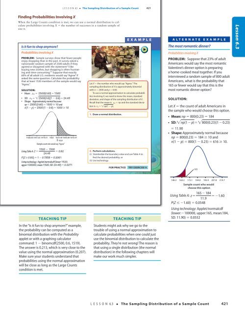Chris Hondros/Getty Images Alternate Example The most romantic dinner? Probabilities involving X PROBLEM: Suppose that 23% of adult Americans would say the most romantic Valentine’s dinner option is preparing a home-cooked meal together. If you interviewed a random sample of 800 adult Americans, what is the probability that 165 or fewer would say that this is the most romantic dinner option? SOLUTION: Let X 5 the count of adult Americans in the sample who would choose this option. • Mean: np 5 800(0.23) 5 184 • SD: "np(1 − p)= "800(0.23)(1 − 0.23) = 11.90 • Shape: Approximately normal because np 5 800(0.23) 5 184 ≥ 10 and n(1 2 p) 5 800(1 2 0.23) 5 616 ≥ 10. 165 Lesson 6.3 18/08/16 5:01 PMStarnes_3e_CH06_398-449_Final.indd 421 Teaching Tip In the “Is it fun to shop anymore?” example, the probability can be computed as a binomial distribution with the Probability applet or with a graphing calculator command: 1 2 binomcdf(2500, 0.6, 1519). The answer is 0.213, which is very close to the value using the normal approximation (0.207). Make sure your students understand that probabilities using the normal approximation will be close as long as the Large Counts condition is met. Teaching Tip 18/08/16 5:01 PM Students might ask why we go to the trouble of using a normal approximation to calculate probabilities when one could just use the binomial distribution to calculate the probability. They’re not wrong! The reason is that using a single distribution (the normal distribution) in the following chapters will make our work much simpler. 148.3 160.2 172.1 184.0 195.9 207.8 219.7 Sample count who would choose this option 165 − 184 Using Table A: z = = −1.60 11.9 P(Z ≤ 21.60) 5 0.0548 Using technology: Applet/normalcdf (lower:2100000, upper:165, mean:184, SD: 11.90) 5 0.0552 L E S S O N 6.3 • The Sampling Distribution of a Sample Count 421 Starnes_3e_ATE_CH06_398-449_v3.indd 421 11/01/17 3:55 PM
Page 2 and 3: 6 Sampling Distributions Please rea
Page 4 and 5: Promoting Good Habits and Skills Ch
Page 6 and 7: Chapter 6 Resources SPA Applets hig
Page 8 and 9: PD Chapter 6 Overview Watch the cha
Page 10 and 11: PD LESSONS 6.1-6.3 Overview Watch t
Page 12 and 13: 402 C H A P T E R 6 • Sampling Di
Page 22 and 23: dd dd d d dddddd 412 C H A P T E R
Page 34 and 35: Answers continued 16. No; assuming
Page 42 and 43: Answers continued X 18. (c) p^ = n
Page 50 and 51: Activity answers continued 3. Yes,
Page 54 and 55: 9. (a) Because n = 50 ≥ 30, the s

SPA 3e_ Teachers Edition _ Ch 6

Create successful ePaper yourself

Delete template?

Save as template?