SPA 3e_ Teachers Edition _ Ch 6

418
C H A P T E R 6 • Sampling Distributions
Teaching Tip
The rule of thumb mentioned here is
sometimes called the 10% condition. As
long as the sample size is less than 10%
of the population size, the sample count
will have a distribution that is close
enough to a binomial distribution that
binomial probabilities will be reasonably
accurate.
Teaching Tip
Remind students that the mean is also
called the expected value!
In practice, we can ignore the violation of the independence condition caused by
sampling without replacement whenever the sample size is relatively small compared
to the population size. Specifically, we can assume that the sampling distribution of a
sample count X is approximately binomial when the sample size is less than 10% of
the population size.
Center and Variability
Because the sampling distribution of a sample count X is approximately binomial
when the sample is a small fraction of the population, we can use the formulas from
Lesson 5.4 to calculate the mean and standard deviation of X.
How to Calculate μ x and σ x for a Binomial Distribution
Suppose X is the number of successes in a random sample of size n from a large population
with proportion of successes p. Then:
• The mean of the sampling distribution of X is m X = np.
• The standard deviation of the sampling distribution of X is s X = "np(1 − p).
The formula for the mean is always correct, even if we are sampling without
replacement. However, the formula for the standard deviation is not appropriate to
use when the sample size is more than 10% of the population size.
Alternate Example
Rubber ducky, are you the one?
Mean and SD of the sampling
distribution of X
PROBLEM: A popular carnival game
has players choose a rubber duck from
a small pool and look under the duck.
If a special mark is on the duck, the
player wins a prize. Suppose that a pool
has 5000 ducks, 800 of which have the
special mark. One generous father pays
for his children to choose 20 rubber
ducks. Let X 5 the number of ducks with
the mark in the sample of 20.
(a) Calculate the mean and standard
deviation of the sampling distribution of X.
(b) Interpret the standard deviation
from part (a).
a
e XAMPLe
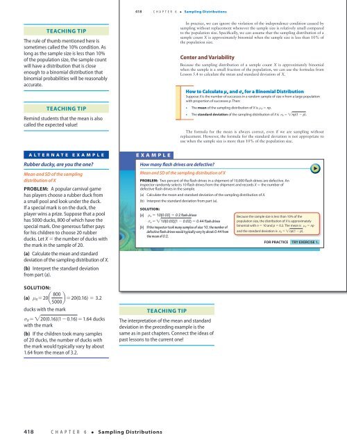
How many flash drives are defective?
Mean and SD of the sampling distribution of X
PROBLEM: Two percent of the flash drives in a shipment of 10,000 flash drives are defective. An
inspector randomly selects 10 flash drives from the shipment and records X 5 the number of
defective flash drives in the sample.
(a) Calculate the mean and standard deviation of the sampling distribution of X.
(b) Interpret the standard deviation from part (a).
SOLUTION:
(a) m x = 10(0.02) = 0.2 flash drives
s x = "10(0.02)(1 − 0.02) = 0.44 f lash drives
(b) If the inspector took many samples of size 10, the number of
defective flash drives would typically vary by about 0.44 from
the mean of 0.2.
Because the sample size is less than 10% of the
population size, the distribution of X is approximately
binomial with n 5 10 and p 5 0.2. The mean is m X = np
and the standard deviation is s X = "np(1 − p).
FOR PRACTICE TRY EXERCISE 1.
SOLUTION:
(a) m X = 20a 800 b = 20(0.16) = 3.2
5000
ducks with the mark
s X = "20(0.16)(1 − 0.16) = 1.64 ducks
with the mark
(b) If the children took many samples
of 20 ducks, the number of ducks with
the mark would typically vary by about
1.64 from the mean of 3.2.
Starnes_3e_CH06_398-449_Final.indd 418
Teaching Tip
The interpretation of the mean and standard
deviation in the preceding example is the
same as in past chapters. Connect the ideas of
past lessons to the current one!
18/08/16 5:00 PMStarnes_3e_CH0
418
C H A P T E R 6 • Sampling Distributions
Starnes_3e_ATE_CH06_398-449_v3.indd 418
11/01/17 3:55 PM